Time evolution of the linear perturbations of a rotating Newtonian polytrope

Abstract

We present the results of numerical time evolutions of the linearised perturbations of rapidly and rigidly rotating Newtonian polytropes while making the Cowling approximation. The evolution code runs stably for hundreds of stellar rotations, allowing us to compare our results with previously published eigenmode calculations, for instance the f-mode calculations of Ipser & Lindblom, and the r-mode calculations of Karino et al. The mode frequencies were found to be in agreement within the expected accuracy. We have also examined the inertial modes recently computed by Lockitch & Friedman, and we were able to extend their slow-rotation results into the rapid rotation regime. In the longer term, this code will provide a platform for studying a number of poorly understood problems in stellar oscillation theory, such as the effect of differential rotation and gravitational radiation reaction on normal mode oscillations and, with suitable modifications, mode-mode coupling in the mildly non-linear regime.

1 Introduction

The study of the normal modes of stars has long been recognised as a subject of considerable importance. The electromagnetic signatures of such oscillations have been used for decades to probe the structure of main sequence stars (Cox 1980). More recently the modes of compact stars (neutron stars and white dwarfs) have received attention from theorists, again with a hope of converting observations into constraints on stellar structure. Such modes may have electromagnetic signatures (van Horn 1980), excited perhaps during accretion or in a thermonuclear burst (Van der Klis 2000). Equally, an oscillating compact star is a source of gravitational radiation, and may even be unstable to such an energy loss via the so-called Chandrasekhar-Friedman-Schutz mechanism (hereafter CFS; see Friedman & Schutz 1978a,b). Particularly in this last regard, it is rapidly rotating compact stars that are of most interest, as only in the case of rapid rotation might gravitational radiation reaction overcome the dissipative effects of viscosity to amplify a mode.

Very few previous studies have examined modes of rapidly rotating compact stars in Newtonian theory (see Stergioulas 1998, Andersson & Kokkotas 2001 for reviews of relativistic computations). The f-modes were calculated by Ipser & Lindblom (1990), the r-modes by Karino et al. (2000), and the inertial modes by Lockitch & Friedman (1999). All of these calculations were carried out by means of an eigenmode analysis, i.e. by assuming an oscillatory constant-frequency solution. In contrast, in this paper we will perform time evolutions of the linearised equations of motion of a rigidly rotating Newtonian polytrope to investigate oscillatory behaviour in the time domain. This will allow us to check, as accurately as a time evolution approach permits, the f-mode, r-mode and inertial-mode frequencies and eigenfunctions in the literature, and also to extend the calculation of the inertial mode frequencies into the regime of rapid rotation. Our work is in much the same spirit as that of Papaloizou & Pringle (1980), who performed time evolutions of r-modes in rapidly rotating thin shells.

Our long-term aim is to provide a stable and well-tested platform for developing a more advanced time evolution code, capable of evolving more realistic stellar models. For instance, future modifications will include evolving a star with a differentially rotating background. This issue is of particular interest, as recently there has been speculation that no mode resembling an r-mode will exist in a sufficiently strongly differentially rotating star (Karino et al. 2000). By starting with a rigidly rotating configuration, and tracking the frequency of a r-mode through a series of runs where the degree of differential rotation is increased step-by-step, it should be possible to probe the mode structure in highly differentially rotating stars.

Another problem that could be addressed using our code is that of modelling gravitational radiation reaction as a local force, included in the equations of motion. A number of elegant formulations of this problem have been presented (see Blanchet et al. 1990 and Rezzolla et al. 1999), but have yet to be fully applied to the modes of compact stars. Recently, Lindblom, Tohline & Vallisneri (2001) included radiation reaction in their evolutions of the r-modes using formulae from Rezzolla et al.  but made some approximations when calculating the force. With our computationally less intensive linear code one can attempt to compare the results obtained via their approximate treatment with those obtained from the full formalism, before the mode saturates due to nonlinear effects..

Another future modification of our code could be to include the first post-Newtonian corrections to the equilibrium star and the equations of motion. This problem is also of considerable interest, as recently Ruoff & Kokkotas (2001) have suggested that r-modes will not exist in sufficiently compact relativistic neutron stars. They speculate that this is due to frame dragging, an effect which is present at first post-Newtonian order. This hypothesis could be tested using a strategy similar to that described above for differential rotation; specifically by performing a series of evolutions of successively more and more compact stars, tracking the r-mode between each evolution.

The implementation of all of these pieces of physics are challenging, and we hope to learn how to deal with each separately in the linear regime before combining them or extending them to the non-linear regime. In essence, our strategy is a modular one, with each problem being isolated and studied on its own. (As regards non-linear evolutions, by coupling several linear time evolution codes it will be possible to monitor mode-mode coupling in the weakly non-linear regime).

In this paper we postpone such advanced calculations, and present evolutions of rigidly rotating Newtonian polytropes, with the perturbations in the gravitational potential neglected (the Cowling approximation). Our goal is to demonstrate the accuracy and stability of our code prior to studying the more complicated physical problems discussed above. We begin by describing some of the computational details (section 2) before examining the f-modes (section 3.1), the r-modes (section 3.2) and finally inertial modes (section 3.3).

2 Formulation of the problem

2.1 The unperturbed star

The unperturbed rotating stellar structure was calculated using the Hachisu self-consistent field method (Hachisu 1986). The equation of state is given by the usual polytropic form:

$$P=K\rho^{\gamma},$$ (1)

where $P$ and $\rho$ denote pressure and density, while $K$ and $\gamma$ are constants. The polytropic exponent $\gamma$ is related to the polytropic index $n$ by

$$\gamma=1+1/n.$$ (2)

Each equilibrium model is characterised by its central density and ratio of the polar to equatorial axes. In constructing an equilibrium model, the equations governing the gravitational potential and the hydrostatic equilibrium are solved iteratively in an integral form (starting from a non-rotating model) until convergence to a desired numerical accuracy is achieved. Our code reproduces the numerical models in Hachisu (1986) to the number of significant digits published.

We will find it useful to introduce a coordinate system consisting of the usual spherical polar $\theta$ and $\phi$ coordinates, but with a modified radial coordinate $x=x(r,\theta)$ which is fitted to surfaces of constant pressure of the background star. With this choice, the unperturbed pressure and density are functions of $x$ only, i.e. $P=P(x)$ and $\rho=\rho(x)$. The usual spherical polar partial derivatives can then be written as:

$$\left.\frac{\partial}{\partial r}\right|_{\theta} = \left.\frac{\partial x}{\partial r}\right|_{\theta}\left.\frac{\partial}{\partial x}\right|_{\theta},$$ (3)

$$\left.\frac{\partial}{\partial\theta}\right|_{r} = \left.\frac{\partial x}{\partial\theta}\right|_{r}\left.\frac{\partial}{\partial x}\right|_{\theta}+\left.\frac{\partial}{\partial\theta}\right|_{x}.$$ (4)

We will choose to set $x$ equal to $r$ in the equatorial plane, i.e. $x(r,\pi/2)=r$. For $\theta<\pi/2$, the oblate shape of the star will mean that $x(r,\theta)>r$. The partial derivatives of $x$ with respect to $r$ and $\theta$ can be easily evaluated using:

$$\left.\frac{\partial x}{\partial r}\right|_{\theta}=\left.\frac{\partial\rho}{\partial r}\right|_{\theta}\left/\frac{\partial\rho}{\partial r}\right|_{\theta=\pi/2},$$ (5)

$$\left.\frac{\partial x}{\partial\theta}\right|_{r}=\left.\frac{\partial\rho}{\partial\theta}\right|_{r}\left/\frac{\partial\rho}{\partial r}\right|_{\theta=\pi/2}.$$ (6)

This choice of coordinate system will make it particularly easy to implement the outer boundary conditions described in section (2.3).

2.2 Equations to be solved

For a given background star, three pieces of physics are required to describe this problem: The equations of motion, the equation of mass conservation, and an equation of state for the perturbations.

The equations of motion referred to the frame of the rotating background are:

$$\frac{\partial{\bf v}}{\partial t}+({\bf v}\cdot\nabla){\bf v}+2{\bf\Omega}\times{\bf v}+{\bf\Omega}\times({\bf\Omega\times r})$$

$$\hskip 142.26378pt=-\frac{1}{\rho}\nabla P-\nabla\phi,$$ (7)

where $\bf v$ denotes the departure of the fluid from the rigid rotation of the background equilibrium model. Performing an Eulerian perturbation and making the Cowling approximation leads to:

$$\frac{\partial{\bf v}}{\partial t}+2{\bf\Omega}\times{\bf v}=\frac{\delta\rho}{\rho^{2}}\nabla P-\frac{1}{\rho}\nabla\delta P.$$ (8)

The prefix $\delta$ denotes an Eulerian perturbation, while $\rho$ and $P$ refer to the background star. The equation of continuity is:

$$\frac{\partial\rho}{\partial t}+\nabla\cdot(\rho{\bf v})=0$$ (9)

which linearises to give:

$$\frac{\partial\delta\rho}{\partial t}+\nabla\cdot(\rho{\bf v})=0.$$ (10)

We will write the equation of state for the perturbations as:

$$\frac{\Delta P}{P}=\gamma_{\rm pert}\frac{\Delta\rho}{\rho},$$ (11)

where $\Delta$ denotes a Lagrangian perturbation. Using the relation that, for a displacement vector ${\bf\xi}$, the Lagrangian and Eulerian perturbations of a scalar are related by

$$\Delta=\delta+\mn@boldsymbol{\xi}\cdot\nabla$$ (12)

we find:

$$\frac{\delta\rho}{\rho}=\frac{1}{\gamma_{\rm pert}}\frac{\delta P}{P}-\mn@boldsymbol{\xi}\cdot{\bf A}.$$ (13)

The vector $\bf A$ is given by:

$${\bf A}=\nabla\log\rho-\frac{1}{\gamma_{\rm pert}}\nabla\log P,$$ (14)

and its magnitude is known as the Schwarzschild discriminant, which depends upon the background pressure and density, and on the index $\gamma_{\rm pert}$ describing the perturbations. We will consider the case where the perturbations obey the same equation of state as the background, so that $\gamma_{\rm pert}=\gamma$ and

$${\bf A}=0.$$ (15)

As discussed in the stellar oscillation literature (see e.g. Tassoul [1978] or Unno et al. [1989]), the magnitude and direction of ${\bf A}$ determines the nature of g-modes in the star. If ${\bf A}$ points inwards the star has stable oscillatory g-modes, while if ${\bf A}$ points outwards the g-modes are unstable, and the star is described as being ‘convectively unstable’. In choosing ${\bf A=0}$ there exists no restoring force at all for g-mode type displacements, so we have eliminated the g-modes altogether from the stellar spectrum.

Expressed in terms of $\delta P$, equations (8) and (10) become:

$$\frac{\partial{\bf v}}{\partial t}+2{\bf\Omega}\times{\bf v} = \frac{\nabla P}{\rho}\frac{1}{\gamma}\frac{\delta P}{P}-\frac{1}{\rho}\nabla\delta P,$$ (16)

$$\frac{\partial\delta P}{\partial t} = -\frac{\gamma P}{\rho}\nabla\cdot(\rho{\bf v}).$$ (17)

With respect to the standard spherical polar vector basis $[\bf{e_{r},e_{\theta},e_{\phi}}]$ (not the coordinate vector basis) we then find:

$$\frac{\partial f_{r}}{\partial t} = -\frac{\partial\delta P}{\partial r}+2\Omega\sin\theta f_{\phi}+\frac{\partial P}{\partial r}\frac{1}{\gamma}\frac{\delta P}{P},$$ (18)

$$\frac{\partial f_{\theta}}{\partial t} = -\frac{1}{r}\frac{\partial\delta P}{\partial\theta}+2\Omega\cos\theta f_{\phi}+\frac{1}{r}\frac{\partial P}{\partial\theta}\frac{1}{\gamma}\frac{\delta P}{P},$$ (19)

$$\frac{\partial f_{\phi}}{\partial t} = -\frac{1}{r\sin\theta}\frac{\partial\delta P}{\partial\phi}-2\Omega(\cos\theta f_{\theta}+\sin\theta f_{r}),$$ (20)

$$\frac{\partial\delta P}{\partial t} = -\frac{\gamma P}{\rho}\nabla\cdot{\bf f}.$$ (21)

where the velocity $\bf v$ has been replaced by the flux ${\bf f}=\rho\bf v$, as this choice of variable leads to very simple outer boundary conditions (see section 2.3).

We follow Papaloizou & Pringle (1980) in decomposing any given perturbation as a sum over basis functions of the form $\cos m\phi$ and $\sin m\phi$, where $m$ is an integer, e.g. for the pressure:

$$\delta P(t,r,\theta,\phi)=\sum_{m=0}^{m=+\infty}\delta P^{+}_{m}(t,r,\theta)\cos{m\phi}$$

$$\hskip 113.81102pt+\delta P^{-}_{m}(t,r,\theta)\sin{m\phi}.$$ (22)

This allows us to reduce the number of space dimensions that appear in the numerical evolution from three to two. With the understanding that the perturbation variables are now functions of $(t,r,\theta)$, but not $\phi$, equations (18)–(21) then apply to each azimuthal number $m$ separately, i.e. the equations decouple in $m$, giving a total of eight equations. The partial derivatives with respect to $\phi$ are trivial to calculate analytically. In summary, equations (18)–(21) then give a set of eight coupled first order linear partial differential equations in the eight unknowns $(\delta P^{+},\delta P^{-},f_{r}^{+},f_{r}^{-},f_{\theta}^{+},f_{\theta}^{-},f_{\phi}^{+},f_{\phi}^{-})$.

For a perturbation of definite azimuthal number $m$, this decomposition with respect to $\phi$ greatly reduces the memory storage and running time of the code, as compared to a fully three-dimensional computation. The fundamental reason that the equations decoupled is that the background star is axisymmetric. A further decomposition in which the $\theta$ dependence of the perturbation variables is written in terms of a set of spherical harmonic functions $Y_{lm}$ is not very useful—the non-spherical nature of the rotating unperturbed star would couple terms with different $l$ indices, with the coupling becoming stronger the more rapidly the star rotates. By eliminating only the $\phi$ dependence, we have simplified the computational costs of the problem to the maximum extend possible without significantly increasing the complexity of the equations to be solved.

2.3 Boundary conditions

By definition, the Lagrangian perturbation in the pressure is zero at the surface, i.e.

$$\delta P+\mn@boldsymbol{\xi}\cdot\nabla P=0{\rm\hskip 28.45274pt(at\,surface).}$$

For the unperturbed star, equation (7) gives:

$$\nabla P=-\rho{\bf\Omega}\times({\bf\Omega\times r})-\rho\nabla\phi.$$ (23)

For a polytrope $\rho=0$ at the surface, from which it follows that $\nabla P=0$ at the surface. It follows at once that our outer boundary condition is:

$$\delta P=0{\rm\hskip 28.45274pt(at\,surface).}$$ (24)

Our choice of coordinates makes imposing the outer boundary condition very simple: We have $\delta P(x=R)=0$, where $R$ denotes the equatorial radius. Also, the mass flux ${\bf f}=\rho{\bf v}$ is zero at the surface, by virtue of the vanishing density, and so

$${\bf f}={\bf 0}{\rm\hskip 28.45274pt(at\,surface).}$$ (25)

Our choice of surface fitted coordinates and perturbation variables guarantees that we never need to evolve quantities at the surface of the star. Numerically, this is highly desirable, as resolving the possibly rapidly falling density profile near the surface can lead to inaccuracies and instabilities.

As we will consider perturbations with $m>0$ we can set $\bf f=0$ at the centre.

3 Results

Equations (18)–(21), decomposed with respect to $\phi$ as described above (equation [22]) were propagated forward in time using the two-step Lax-Wendroff scheme described in Press et al. (1986). The code is second order convergent, and runs stably for hundreds of rotation periods. The second order convergence is illustrated by figure 1. In this figure we plot the total kinetic energy of the star, as measured in the rotating frame, as a function of time for some arbitrary initial data. The time is given in units of $1/\sqrt{\pi G\rho_{0}}$, where $\rho_{0}$ is the average density of the non-rotating star of the same mass and equation of state. The star rotates at a rate $\Omega/\sqrt{\pi G\rho_{0}}=0.538$, corresponding to a polar-to-equatorial axis ratio of $0.79$. The evolution was performed for three different grid resolutions, labelled as high, medium and low in the figure, with the resolution differing by a factor of two between each successive run. In full, for the high resolution run we used a grid of $64$ angular points by $60$ radial ones, the medium resolution grid was $32$ by $30$ points, and the low resolution grid was $16$ by $15$ points. The kinetic energy is normalised to unity at $t=0$. A small oscillation is visible, corresponding to the excitation of a p-mode (Cox 1980), whose exact nature need not concern us here. A convergence ratio $C$ is then calculated as the ratio:

$$C=\frac{E(t,{\rm high\,resolution})-E(t,{\rm low\,resolution})}{E(t,{\rm high\,resolution})-E(t,{\rm medium\,resolution})}$$ (26)

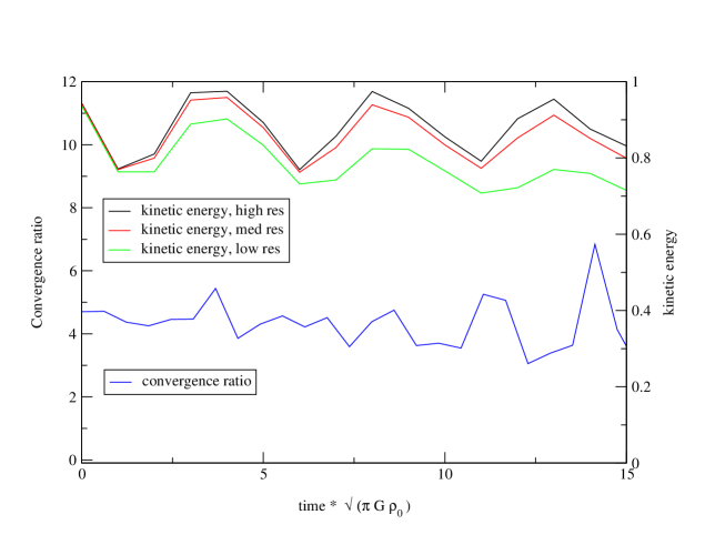
Figure 1: Demonstration of second order convergence. The three upper curves plot the kinetic energy at three different grid resolutions, labelled as high, medium and low resolutions. The lower curve is the dimensionless convergence ratio, defined in equation (26). Time is plotted in unity of $1/\sqrt{\pi G\rho_{0}}$, where $\rho_{0}$ is the average density of the non-rotating star of the same mass.

For a code with second order accuracy in space, the ratio can be shown to be approximately equal to 5. This is indeed the case for our time evolution code. Beyond the time interval shown in the figure, the oscillations in the energy start to loose phase coherence, and the convergence ratio begins to oscillate strongly. The convergence ratio then looses its significance.

The long-term stability of the code is illustrated by figure 2, which plots the kinetic energy of the star as a function of time. The rotation rate is the same as above, and the star rotates $100$ times over the period plotted. A small amount of artificial viscosity was included to give this long-term stability, and the grid consisted of $32$ angular points and $30$ radial ones. The initial data used was that of an $l=m=2$ r-mode for a slowly rotating star (about $80$ r-mode oscillations occur over this interval). A rather sharp loss of kinetic energy occurs over the first ten or so rotations. This is likely due to the initial data exciting a number of short-wavelength modes whose energy was rapidly dissipated. Over the remainder of the evolution, the kinetic energy remains approximately constant, falling by about $10\%$ over the remaining $90$ rotations, confirming the long-term stability of our code. This evolution required approximately two hours of computer time on a standard PC. Most of the results in this paper are based on runs of this duration or less.

Part of the above energy loss is due to the artificial viscosity, and part due to numerical error. Given that the code has been shown to be second order convergent, an increase in grid resolution by a factor of $N$ would reduce the rate of energy loss due to numerical error by a factor $N^{2}$. On the basis of runs we have performed where the artifical viscosity was set to zero, we estimate that an increase in grid resolution by a factor of $10$ (i.e. a $320$ by $300$ grid) would be sufficient to reduce the energy loss to around $1\%$ for an evolution of the above duration. Such a run would take over a week on a standard PC, and so has not been performed here. However, should such a high level of accuracy be required for a particular application, the necessary runs could be easily be done on a supercomputer.

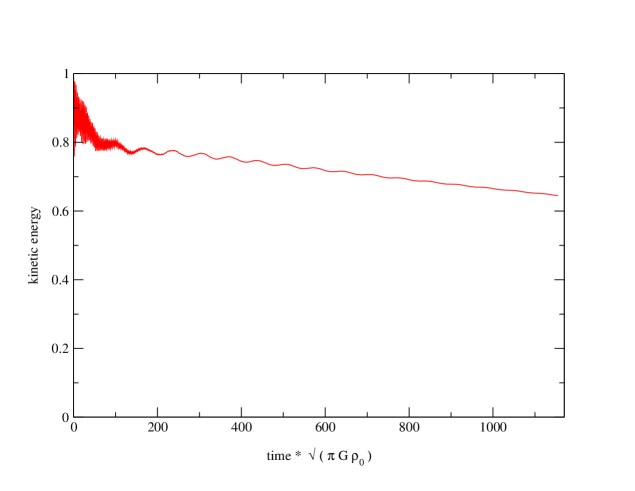
Figure 2: Kinetic energy as a function of time, normalised to unity at $t=0$, and time measured in the same units as in figure 1). Around $100$ stellar rotations occur over the period plotted.

In the following sections we will use this time evolution code to study f-modes, r-modes and inertial modes. We will use as initial data some (possible crude) approximation to the true eigenfunction. The perturbed quantities will then be Fourier analysed. By performing a series of such evolutions, of gradually increasing stellar rotation rate, the mode of interest can then be tracked from the slow-rotation case (where it’s approximate frequency is already known) into the rapid rotation regime.

Note that for an evolution of duration $T$, the error in the frequency localisation of the transform is approximately equal to $1/T$. It was therefore necessary to perform long time evolutions to obtain accurate frequencies. This error in measurement is indicated by error bars on the mode frequency plots that follow (figures 4–8). However, it should be noted that this is not the only source of error—the finite grid resolution will affect the results also, but its effect is not as easy to quantify. The error bars in the figures should be regarded as simple estimates of the error.

Note that all mode frequencies given in this paper are measured in the rotating frame. Also, we only present results for the case when the polytropic index $n$ is equal to unity.

3.1 The f-modes

As described above, to investigate a particular mode it was necessary to supply our code with initial data that would excite it. In the case of f-modes we chose to use initial data of the form:

$$\delta P=\rho\left(\frac{r}{R(\theta)}\right)^{l}Y_{ll},$$ (27)

where $R(\theta)$ denotes the stellar radius at polar angle $\theta$ and $Y_{ll}$ is a spherical harmonic. This reduces to the correct f-mode pressure perturbation in the limit of zero rotation for an incompressible star, in the Cowling approximation. The perturbed mass flux $\bf f$ was set to zero in the initial data. The mode frequency was then extracted by taking power spectra of the time series of the perturbed quantities. A more efficient excitation of the f-modes would have been possible if non-zero initial data was provided for $\bf f$ also, but this was not found to be necessary—the f-modes were easily identifiable using the above initial data. Indeed, this scheme efficiently excited the $l=m$ mode in all but the most rapidly rotating stars.

The power spectra of the evolutions consisted of just one peak for the non-rotating star. This then split into two peaks for $\Omega\not=0$, corresponding to the breaking of the degeneracy between co- and counter-rotating modes. This is illustrated in figure 3 for the spectra of $\delta P^{+}$ for the $l=m=2$ f-mode. The left hand panel was obtained for a non-rotating star, while the right hand one was for a rotating one ($\Omega/\sqrt{\pi G\rho_{0}}=0.37$, polar-to-equatorial radius ratio 0.92). Note how the power in the degenerate $\Omega=0$ peak for the static star is split roughly equally between the co- and counter-rotating peaks in the $\Omega\not=0$ case. As the star’s rotation rate was increased, the frequency separation of the modes increased, and the power was shared less evenly between the two.

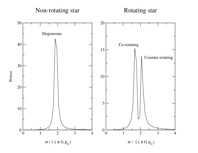
Figure 3: Power spectra of the perturbed pressure $\delta P^{+}$ for a non-rotating star (left panel) and for a rotating star (right panel). The powers are in the same (arbitrary) units in both panels, while the mode frequencies are in units of $\sqrt{\pi G\rho_{0}}$, as indicated.

Before examining the case of rotating stars in detail we will consider the simpler case of non-rotating ones. The mode frequencies, as calculated by a normal mode analysis in the Cowling approximation (Kokkotas, personal communication), are given in table 1 for the $l=m=2$, $4$ and $6$ modes. Also shown are the mode frequencies we obtained from our time evolution code, and the percentage difference between the two. In this non-rotating case the eigenmode calculation is known to be highly accurate, so that the percentage differences in the table give an indication of the accuracy of our code. The difference is very small (less than $1\%$) in the $l=m=2$ case, but somewhat higher (around $4\%$) for the high-index modes. This decrease in accuracy is almost certainly due the higher-index modes varying on smaller length scales than the $l=m=2$ mode, and therefore being less well represented on our spatial grid.

$l=m=$	$2$	$4$	$6$
Eigenmode	$1.912$	$2.577$	$3.077$
Time evolution	$1.90$	$2.68$	$2.96$
Percentage difference	$0.5$	$3.8$	$3.9$

Table 1: F-mode frequencies as calculated by an eigenmode analysis, and using our time evolution code (units same as in figure 3). The eigenmode vales are anticipated to be of high precision, so that the percentage difference between the two is an indication of the accuracy of our time evolutions.

We then investigated f-modes in rotating stars. The f-mode eigenfrequencies and eigenfunctions of rapidly rotating stars have been calculated by Ipser & Lindblom (1990), without making the Cowling approximation. Specifically, they considered polytropic stars, and searched for modes which had spherical harmonic indices $l=m$ in the limit of slow rotation.

The frequency of the co- and counter-rotating modes, together with the Ipser & Lindblom values for the counter-rotating mode, are plotted in figures 4, 5 and 6, for $l=m=2,4,6$ respectively.

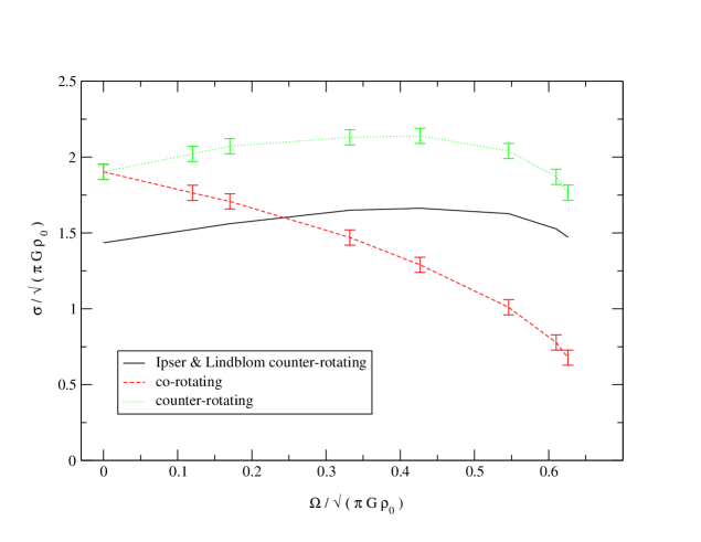
Figure 4: The $l=m=2$ f-mode frequencies as a function of rotation rate. The upper curve is for the counter-rotating mode as calculated by our time evolution code. This is to be compared with the Ipser & Lindblom result of the solid curve. The difference between the two results is due to our having made the Cowling approximation. The monotonically decreasing curve is the co-rotating mode frequency as calculated by our code. All frequencies are in units of $\sqrt{\pi G\rho_{0}}$, where $\rho_{0}$ is the average density of the non-rotating star of the same mass and equation of state. In these units, the Kepler rotation rate is 2/3.

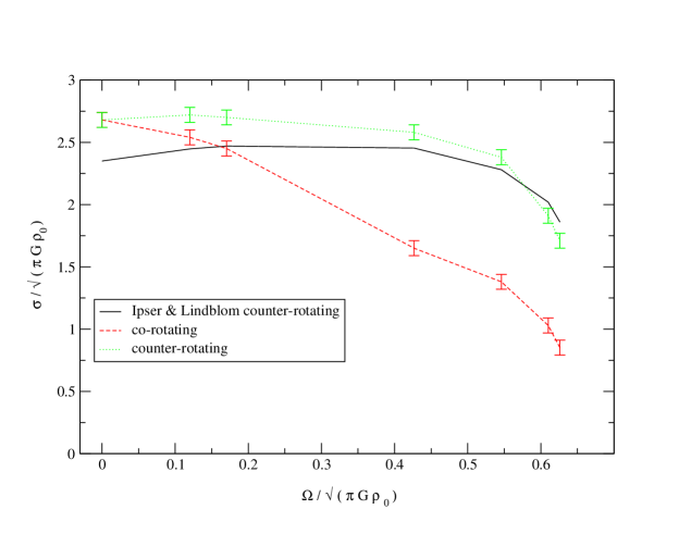
Figure 5: As figure 4, with $l=m=4$

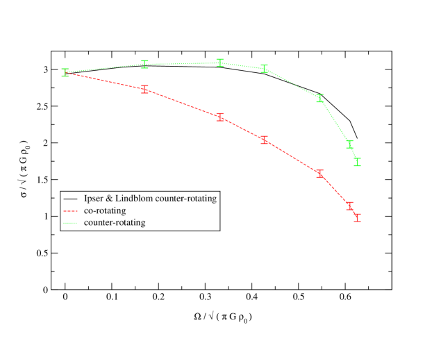
Figure 6: As figure 4, with $l=m=6$

For most rotation rates the counter-rotating mode frequencies calculated from our time evolutions are somewhat higher than those calculated by Ipser & Lindblom. This is almost certainly due to our having made the Cowling approximation, while Ipser & Lindblom have not. The discrepancy is typically of order 30% for $l=m=2$, 10% for $l=m=4$ and 3% for $l=m=6$. Such a decrease of discrepancy with increasing harmonic index is to be expected: higher order modes have alternating regions of positive and negative density perturbation, whose contribution to the perturbation in the gravitational potential at a given point tend to cancel one-another out (Cowling 1941). We can therefore conclude that, within the error margin of the Cowling approximation, our time evolution code confirms the f-mode frequencies calculated by Ipser & Lindblom.

3.2 The r-modes

Because of the considerable interest aroused by the r-modes (see Andersson & Kokkotas 2001 for a recent review), we used our time evolution code to examine both the frequencies and eigenfunctions of this class of mode. For initial data we provided a perturbation in the mass flux of the form:

$${\bf f}=\rho\left(\frac{r}{R(\theta)}\right)^{l}{\bf Y^{B}}_{ll},$$ (28)

where ${\bf Y^{B}}_{ll}$ is a magnetic spherical harmonic (Thorne 1980). In the limit of slowly rotating stars, this becomes an exact mode solution of the linearised equations of motion.

3.2.1 The r-mode frequencies

In order to extract r-mode frequencies, the power spectra of the $\theta$ and $\phi$ components of the mass flux were analysed. The result of a series of such evolutions for the $l=m=2$ r=mode is shown in figure 7, with the error bars indicating the uncertainty in the frequency. On the vertical axis we plot the dimensionless ratio $\sigma/\Omega$, where $\sigma$ is the mode frequency. On the horizontal axis we plot the normalised rotation rate $\Omega/\sqrt{\pi G\rho_{0}}$.

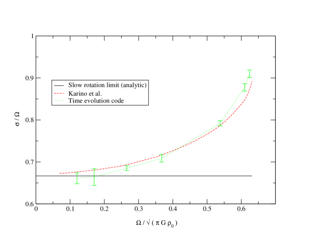
Figure 7: The frequency of the $l=m=2$ r-mode as a function of rotation rate. Mode frequencies are given in units of $\Omega$, the stellar rotation rate. As in previous plots, the error bars indicated the result of our time evolution code. The dotted line gives the mode frequency calculated by Karino et al. (2000). The horizontal line indicates the analytic slow rotation limit of 2/3.

For comparison, a curve showing the mode frequency as calculated by Karino et al. (2000) is shown also, together with a horizontal line at the mode frequency as calculated using the slow rotation limit ($\sigma/\Omega=2/3)$. Note that Karino et al. did not make the Cowling approximation. Within the indicated uncertainties due to the finite duration of the time evolution, the data sets agree very well, even at the fastest rotation rates. To leading order in the rotation rate, the Cowling approximation is known to not affect the mode frequency, so this close agreement was to be expected. There is a slight difference between our results and those of Karino et al. at the highest rotation rates. We suspect this is due to the Cowling approximation being a poorer approximation in this regime, as the fractional density perturbation $\delta\rho/\rho$ is known to increase with rotation rate as $\Omega^{2}$ for r-modes (Andersson & Kokkotas 2001).

3.2.2 The r-mode eigenfunctions

The r-mode eigenfunctions were calculated by Karino et al. (2000). In order to confirm their veracity, these eigenfunctions were used as initial data for our time evolutions. An accurate eigenfunction would excite the appropriate r-mode only, with little excitation of other modes, while an inaccurate function would deposit a significant quantity of energy over other modes. In order to quantify this, we examined the power spectra of several evolutions with different stellar rotation rates, for the $l=m=2$ r-mode. For each evolution we noted the ratio of the r-mode excitation peak to the next strongest excitation.

We found that in the power spectra of $f_{\theta}$ and $f_{\phi}$, the r-mode excitation was extremely clean, so that secondary peaks are many orders of magnitude smaller. For $f_{r}$ and $\delta p$ significant secondary peaks were present, implying that our initial data also excited some radial modes or polar modes of oscillation. The ratios of these to the r-mode peak are given in table 2, for stars with rotation rates $\Omega/\sqrt{\pi G\rho_{0}}$ of $0.170$, $0.538$ and $0.624$.

$\sigma/\sqrt{\pi G\rho_{0}}=$	$0.170$	$0.538$	$0.624$
	Peak ratio
$f_{r}^{+}$	224	42.6	4.26
$\delta P^{+}$	7740	174	8.06

Table 2: Ratio of $m=2$ r-mode excitation peak to next strongest peak (representing other modes), for the quantities $f_{r}^{+}$ and $\delta P^{+}$, for three different rotation rates. Recall than the Kepler rotation rate is $2/3$ in these units.

Clearly, in all cases the initial data efficiently picks out the r-mode from the stellar spectrum. The excitation is more accurate the slower the rotation of the star, but even in the the rapidly rotating $\Omega/\sqrt{\pi G\rho_{0}}=0.624$ case there is little other mode excitation. The kinetic energy of the perturbations is quadratic in the mass flux, so that in this case only a few percent of the kinetic energy of the initial data is deposited into modes other than the r-mode. For the relatively slowly rotating $\Omega/\sqrt{\pi G\rho_{0}}=0.170$ case, only a few thousandths of a percent is deposited. We can therefore confirm that the eigenfunctions computed by Karino et al. (2000) are accurate.

3.3 Inertial modes

The r-modes of the previous section are a special case of a wider class of oscillations, known as inertial modes (Greenspan 1968, Pedlosky 1987). The defining feature of the inertial modes is that their frequency vanishes linearly in the limit of zero stellar rotation, or equivalently that $\sigma/\Omega$ remains finite in this limit. The r-modes of the last section are the subset of the inertial modes which have purely axial velocity perturbations in the limit of zero rotation (axial means that the velocity can be written in terms of $\nabla\times Y_{lm}$). Furthermore, for stars with zero Schwarzchild discriminant, the two spherical harmonic indices of the r-modes must be equal, i.e. $l=m$ (Provost et al. 1981).

In contrast, inertial modes are hybrid, having velocity perturbations with both axial and polar parts, even in the slow rotation limit (polar means that the velocity field can be written as a sum of terms proportional to $Y_{lm}{\bf e}_{r}$ and $\nabla Y_{lm}$). Also, the inertial modes are not restricted to $l=m$ spherical harmonics. Inertial modes were considered in detail recently by Lockitch & Friedman (1999), who calculated mode frequencies and eigenfunctions. It was found that many of these inertial modes could undergo the CFS instability and are therefore interesting from a gravitational wave point of view, even though they are probably not as strongly unstable as the $l=m=2$ r-mode. It is therefore of interest to extend the calculations of Lockitch & Friedman and calculate these mode frequencies for more rapidly rotating stars.

We have performed such an analysis using our time evolution code. We used the analytic approximations to eigenfunctions given by Lockitch & Friedman as initial data to carry out evolutions of several inertial modes.

A graph showing the frequency of three such modes as a function of stellar rotation rate is shown in figure 8. These are $m=2$ modes whose leading contribution to the velocity field has harmonic index $l=4$. Analytic fits to the radial eigenfunctions of these modes in uniform density stars are given in table 3 of Lockitch & Friedman. As the latter authors note, the eigenfunctions are very similar for $n=1$ polytropes, so we have used these analytic functions to supply initial data to our code. As in previous figures, the vertical axis plots the dimensionless mode frequency as measured in the rotating frame, while the angular rotation rate is given in units of $\sqrt{\pi G\rho_{0}}$. The three horizontal lines indicate the mode frequency in the slow rotation limit as calculated by Lockitch & Friedman (see table 6 of their paper).

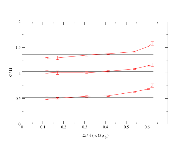
Figure 8: Oscillation frequencies for inertial modes. The three modes all have leading order velocity perturbations proportional to the $l=4$, $m=2$ spherical harmonic in the limit of slow rotation, but have different radial behaviour. The units are the same as in figure 7. The horizontal lines indicate the mode frequencies as calculated by Lockitch & Friedman in the slow rotation non-Cowling limit.

In the limit of slow rotation we found the eigenfunctions were sufficiently accurate to deposit approximately $99\%$ of their energy into a single mode, with frequency very close to that computed by Lockitch & Friedman, confirming our identification of the mode. The slight difference between the frequencies is due to our having made the Cowling approximation, while Lockitch & Friedman have not.

4 Conclusions

In this paper we have presented results from a numerical code for time evolutions of perturbations of rapidly and rigidly rotating Newtonian polytropes (within the Cowling approximation). Our code is second order convergent and runs stably for many (i.e. hundreds) of stellar oscillations. We have compared the results of our evolutions with calculations of f- and r-modes in the literature and found agreement within the errors expected for the Cowling approximation. We have also presented results for the inertial modes, and (for the first time) extended the frequencies calculated by Lockitch & Friedman into the rapid rotation regime.

Even though we have provided some new results for oscillations in stars rotating near the break-up limit, this work is essentially a “proof of principle”. Our main aim was to illustrate the accuracy attainable with a time-evolution approach to the problem of rotating stars. In particular, the relative simplicity and reliability of the perturbative 2D approach makes it a valuable complement to fully 3D hydrodynamical simulations, such as the recent ones by Lindblom, Tohline and Vallisneri (2001).

Having demonstrated the stability and accuracy of our code, we plan to use it as a test-bed for the implementation of additional physical features, which we will add in a modular fashion, one at a time. Via such a gradual escalation in complexity, we hope to arrive at a code capable of evolving rather more realistic stars, incorporating (for instance) differential rotation, gravitational radiation reaction, and non-linear effects. Such extensions are currently underway, and will be presented in due course.

References

- [1]
- [2] Andersson N., Kokkotas K. D., 2001, Int.J.Mod.Phys. D 10 381
- [3]
- [4] Blanchet L., Damour T., Schafer G., 1990, MNRAS 242 289
- [5]
- [6] Cowling T. G., 1941, MNRAS 101 367
- [7]
- [8] Cox J. P., 1980, Theory of Stellar Pulsation, Princeton University Press, Princeton
- [9]
- [10] Friedman J. L., Schutz B. F., 1978a, Ap. J. 221 937
- [11]
- [12] Friedman J. L., Schutz B. F., 1978b, Ap. J. 222 281
- [13]
- [14] Greenspan H.P., 1968, The Theory of Rotating Fluids, Cambridge University Press
- [15]
- [16] Hachisu I., 1986, Ap. J. Suppl. 61 479
- [17]
- [18] Ipser J. R., Lindblom L., 1990, Ap. J. 355 226
- [19]
- [20] Karino S., Yoshida S., Yoshida S., Eriguchi Y., 2000, Phys. Rev. D 62 084012
- [21]
- [22] Lindblom L., Tohline J. E., Vallisneri M., 2001, preprint, astro-ph/0109352
- [23]
- [24] Lockitch K. H., Friedman J. L., 1999, Ap. J. 521 764
- [25]
- [26] Papaloizou J. C., Pringle J. E., 1980, MNRAS 190 43
- [27]
- [28] Pedlosky J., 1987, Geophysical fluid dynamics, Springer Verlag
- [29] Press W. H., Flannery B. P., Teukolsky S. A., Vetterling W. T., 1986, Numerical Recipes, CUP, Cambridge
- [30]
- [31] Provost J., Berthomieu G., Rocca A., 1981, Astron. & Astrophys. 94 126
- [32]
- [33] Rezzolla L., Shibata M., Asada H., Buamgarte T. W., Shapiro S. L., 1999, Ap. J. 525 935
- [34]
- [35] Ruoff J., Kokkotas K. D., 2001, preprint, gr-qc/0106073
- [36]
- [37] Stergioulas N., 1998, Living Rev. Relativity 1 8. Online article: http://www.livingreviews.org/Articles/Volume1/1998-8stergio
- [38]
- [39] Tassoul J-L., 1978, Theory of Rotating Stars, Princeton University Press, Princeton
- [40]
- [41] Thorne K. S., 1980, Rev. Mod. Phys. 52 299
- [42]
- [43] Unno W., Osaki Y., Ando H., Shibashashi H., 1989, Nonradial Oscillations of Neutron Stars, University of Tokyo Press
- [44]
- [45] Van der Klis M., 2000, Annual Rev. Astron. and Astrophys. 38 717
- [46]
- [47] Van Horn H. M., 1980, Ap. J. 236 899
- [48]