Large-scale Correlation of Mass and Galaxies with the Ly$\alpha$ Forest Transmitted Flux

Abstract

We present predictions of the correlation between the Ly$\alpha$ forest absorption in quasar spectra and the mass within $\sim 5\,h^{-1}\,{\rm Mpc}$ (comoving) of the line of sight, using fully hydrodynamic and hydro-PM numerical simulations of the cold dark matter model supported by present observations. The observed correlation based on galaxies and the Ly$\alpha$ forest can be directly compared to our theoretical results, assuming that galaxies are linearly biased on large scales. Specifically, we predict the average value of the mass fluctuation, $<\!\delta_{m}\!>$, conditioned to a fixed value of the Ly$\alpha$ forest transmitted flux $\delta_{F}$, after they have been smoothed over a $10\,h^{-1}\,{\rm Mpc}$ cube and line of sight interval, respectively. We find that $<\!\delta_{m}\!>/\sigma_{m}$ as a function of $\delta_{F}/\sigma_{F}$ has a slope of $0.6$ at this smoothing scale, where $\sigma_{m}$ and $\sigma_{F}$ are the rms dispersions (this slope should decrease with the smoothing scale). We show that this value is largely insensitive to the cosmological model and other Ly$\alpha$ forest parameters. Comparison of our predictions to observations should provide a fundamental test of our ideas on the nature of the Ly$\alpha$ forest and the distribution of galaxies, and can yield a measurement of the bias factor of any type of galaxies that are observed in the vicinity of Ly$\alpha$ forest lines of sight.

1 INTRODUCTION

The prevalent theory to explain the Ly$\alpha$ forest is that the absorption lines arise from density variations in a photoionized intergalactic medium that originate in the gravitational evolution of primordial fluctuations. Both semi-analytic models and numerical simulations (Bi 1993; Cen et al. 1994; Zhang et al. 1995, 1998; Hernquist et al. 1996; Miralda-Escudé et al. 1996; Bi & Davidsen 1997) have shown that the predicted Ly$\alpha$ spectra appear remarkably similar to the observations. The good agreement of the predicted and observed flux distribution and power spectrum of the Ly$\alpha$ forest (Rauch et al. 1997; Croft et al. 1999; McDonald et al. 2000), and the large transverse size of the absorption systems (Bechtold et al. 1994; Dinshaw et al. 1994, 1997; Petitjean et al. 1998; Monier, Turnshek, & Hazard 1999; Dolan et al. 2000; López, Hagen, & Reimers 2000) are the basic tests that have so far been done and have supported the theory. In addition, this Ly$\alpha$ forest theory is derived from the general Cold Dark Matter (hereafter, CDM) model with parameters that are well constrained from several other observations (e.g., Primack 2000).

Another important test of our ideas of the Ly$\alpha$ forest can be done by observing the correlation of the transmitted flux in a spectrum with galaxies. Some of these observations have already been done for small scales and high column density absorbers, which have shown the expected strong correlation between galaxies and gas halos (e.g., Bergeron & Boissé 1991; Steidel, Dickinson, & Persson 1994; Lanzetta et al. 1995; Chen et al. 2001). Penton, Stocke, & Shull (2001) have probed this correlation at low redshift, and have found that the weak absorption lines are often found in low-density regions of the galaxy distribution. Recently, Adelberger et al. (2001) have carried out the first analysis of this correlation on large scales (several comoving Mpc) and at high redshift (using galaxies detected with the Lyman break technique), using the transmitted flux as the quantity to correlate with the mean number of galaxies in a specified region.

Inspired by the observational results of Adelberger et al. (2001), this paper presents detailed theoretical predictions for statistical functions similar to the one introduced by those authors. Namely, we analyze the mean value of the mass given an observed value of the transmitted flux, and the mean value of the transmitted flux for a fixed value of the mass, after both quantities have been smoothed over a certain region. The main difference between the functions we analyze and the function shown by Adelberger et al. (2001) is that the observed objects are of course galaxies, and our simulations predict only the distribution of the mass. However, the predictions of the simulations can still be compared to the galaxy observations to determine the relation between galaxies and mass, which is especially straightforward if linear bias is a sufficient description of the distribution of galaxies relative to the mass on the large scales being probed. We examine the dependence of these statistical functions on the various parameters affecting the Ly$\alpha$ forest in §3.

2 METHOD

We use several HPM (hydro-particle-mesh; see Gnedin & Hui 1998) simulations to model the Ly$\alpha$ forest, after testing that the HPM approximation is sufficient for our purposes by comparing to a fully hydrodynamic simulation. The standard HPM simulations that will be used most often in this paper have box size $40\,h^{-1}\,{\rm Mpc}$, with $512^{3}$ particles. The cosmological model is CDM with cosmological constant, in a flat universe with present matter density $\Omega_{m}=0.4$, power spectrum index $n=0.95$, and amplitude given by $\sigma_{8}=0.75$. All the results in this paper will be shown at $z=3$, the typical redshift at which the observations have so far been done. The model we use is consistent with the observed Ly$\alpha$ forest power spectrum: at the typical Ly$\alpha$ forest scale of $k=0.008~{}(\,{\rm km\,s}^{-1})^{-1}$, it has $\Delta^{2}_{\rho}(k)=0.29$ at $z=3$ [where $\Delta^{2}_{\rho}(k)$ is the contribution per unit $\ln k$ to the variance of the linear theory mass density fluctuations], while the observed value is $\sim 0.26$ (McDonald et al. 2000; Croft et al. 2002). The redshift interval corresponding to $40\,h^{-1}\,{\rm Mpc}$ in this model near $z=3$ is $\Delta z=0.068$. The density-temperature relation assumed for the gas is $T(\Delta)=T_{1.4}(\Delta/1.4)^{\gamma-1}$, where $\Delta$ is the gas density divided by the mean gas density. We use the parameters $T_{1.4}=17000$ K and $\gamma-1=0.3$ in our standard simulation (the reason we specify the value of the temperature $T_{1.4}$ at $\Delta=1.4$ is because the error in the temperature was determined to be smallest at this density in McDonald et al. 2002). Several other similar simulations are used where we vary each one of the relevant parameters (see §3), and we vary also the box size and resolution to verify the numerical convergence of the results. Unless otherwise indicated, all the results we show for a given set of parameters are averages of four simulations with different random initial perturbations.

2.1 Definitions

We define the quantity $\delta_{F}\equiv 1-F/\bar{F}$, where $F$ is the fraction of transmitted flux in the Ly$\alpha$ forest after the spectrum has been smoothed along the line of sight with a filter, and $\bar{F}$ is the mean transmitted flux. We use a Gaussian smoothing filter in this paper, which is $W(kR)=\exp[-(kR)^{2}/2]$ in Fourier space. We also define $\delta_{m}$ as the redshift-space mass density perturbation, again smoothed over a specified region. We choose to smooth the mass fluctuation over cubes of $10\,h^{-1}\,{\rm Mpc}$ (comoving) in redshift space, centered on the Ly$\alpha$ forest line of sight, which is approximately the smoothing that is used in Adelberger et al. (2001). This is convenient to do in observations of galaxies, since galaxies are usually searched for in a square field of view, and they can simply be divided into redshift bins. Note that the size of our cubes in velocity units, $1280\,{\rm km\,s}^{-1}$, is more fundamental than the size in $\,h^{-1}\,{\rm Mpc}$, because the temperature and observed flux power spectrum are both measured in $\,{\rm km\,s}^{-1}$.

In general, the information that can be recovered from observations is the full joint probability distribution $P(\delta_{F},\delta_{g})$, where $\delta_{g}$ is the fluctuation in the number of galaxies. In this paper we present results from HPM numerical simulations for $<\!\delta_{m}|\delta_{F}\!>$, which is the mean value of the mass fluctuation subject to the condition of a fixed value in the transmitted flux fluctuation, and for the analogous quantity $<\!\delta_{F}|\delta_{m}\!>$. The observed galaxies may not follow exactly the same fluctuations as the mass, even when smoothed over a scale of $10\,h^{-1}\,{\rm Mpc}$. However, if galaxies are linearly biased at this large scale, then $\delta_{g}=b\,\delta_{m}$, where $\delta_{g}$ is the fluctuation in the galaxies and $b$ is the bias factor. If we now define the quantity $\tilde{\delta}_{m}=\delta_{m}/\sigma_{m}$, and $\tilde{\delta}_{g}=\delta_{g}/\sigma_{g}$, where $\sigma_{m}$ and $\sigma_{g}$ are the rms fluctuation of $\delta_{m}$ and $\delta_{g}$, then $\tilde{\delta}_{m}=\tilde{\delta}_{g}$ and the correlation with $\delta_{F}$ is precisely predicted. For convenience, we also define the quantity $\tilde{\delta}_{F}=\delta_{F}/\sigma_{F}$, and we will present results for $<\!\tilde{\delta}_{m}|\tilde{\delta}_{F}\!>$ and $<\!\tilde{\delta}_{F}|\tilde{\delta}_{m}\!>$.

2.2 Smoothing

To choose a value of the smoothing radius $R$ for the smoothing filter of the Ly$\alpha$ forest transmitted flux, we compute first the correlation coefficient $<\!\delta_{F}\delta_{m}\!>/\sigma_{F}\sigma_{m}$ in our standard simulation, and show it as a function of $R$ in Figure 1. The correlation is maximum at $R=3.5\,h^{-1}\,{\rm Mpc}$. The dependence of the correlation on $R$ is not surprising: if $R$ is too small, the value of $\delta_{F}$ is altered by small-scale fluctuations that are not related to the value of $\delta_{m}$ and therefore act as noise, and if $R$ is too big, then the fluctuations affecting $\delta_{m}$ are erased by smoothing in the value of $\delta_{F}$.

Figure 1: Correlation between mass and transmitted flux as a function of the smoothing applied on the spectrum, with the Gaussian filter, $W(kR)=\exp[-(kR)/2]$. The squares show the correlation, $<\!\delta_{F}~{}\delta_{m}\!>/(\sigma_{F}~{}\sigma_{m}$).

A Gaussian filter with $R=3.5\,h^{-1}\,{\rm Mpc}$ will be used for the smoothing of the Ly$\alpha$ spectrum throughout the rest of this paper. However, before proceeding, we examine how much our results differ if we use instead a top-hat smoothing for the Ly$\alpha$ spectrum, or if we vary the size of the cube over which the mass is smoothed.

Throughout the paper, our results will be presented as a set of four figures showing the four functions $<\!\delta_{m}|\delta_{F}\!>$, $<\!\delta_{F}|\delta_{m}\!>$, $<\!\tilde{\delta}_{m}|\tilde{\delta}_{F}\!>$, and $<\!\tilde{\delta}_{F}|\tilde{\delta}_{m}\!>$. In all these figures, the function $<\!\delta_{m}|\delta_{F}\!>$ has been obtained by creating spectra along each row of cells in the simulation, smoothing the spectra along the line of sight, selecting all the pixels in the spectra where the value of $\delta_{F}$ is inside a given bin, and computing the average $\delta_{m}$ for these pixels, where $\delta_{m}$ is computed in redshift-space. We use bins of width $\Delta\delta_{F}=0.05$. Similarly, $<\delta_{F}|\delta_{m}>$ is calculated by averaging the values of $\delta_{F}$ for pixels in bins with a given $\delta_{m}$ (again using $\Delta\delta_{m}=0.05$ for the bin width).

Figure 2: Comparison between our standard $3.5\,h^{-1}\,{\rm Mpc}$ Gaussian smoothing of the spectrum with $10\,h^{-1}\,{\rm Mpc}$ cube smoothing of the mass (solid, black line) and $5\,h^{-1}\,{\rm Mpc}$ top-hat smoothing of the spectrum (dotted, red line), $12\,h^{-1}\,{\rm Mpc}$ cube smoothing of the mass with $4.2\,h^{-1}\,{\rm Mpc}$ Gaussian smoothing of the spectrum (long-dashed, green line), or $8\,h^{-1}\,{\rm Mpc}$ cube smoothing of the mass with $2.7\,h^{-1}\,{\rm Mpc}$ Gaussian smoothing of the spectrum (short-dashed, blue line). (a) mean mass as a function of transmitted flux, (b) mean flux as a function of mass, (c and d) are as (a and b) except that $\delta_{F}$ and $\delta_{m}$ are divided by their rms fluctuation. The mass is always computed in redshift space.

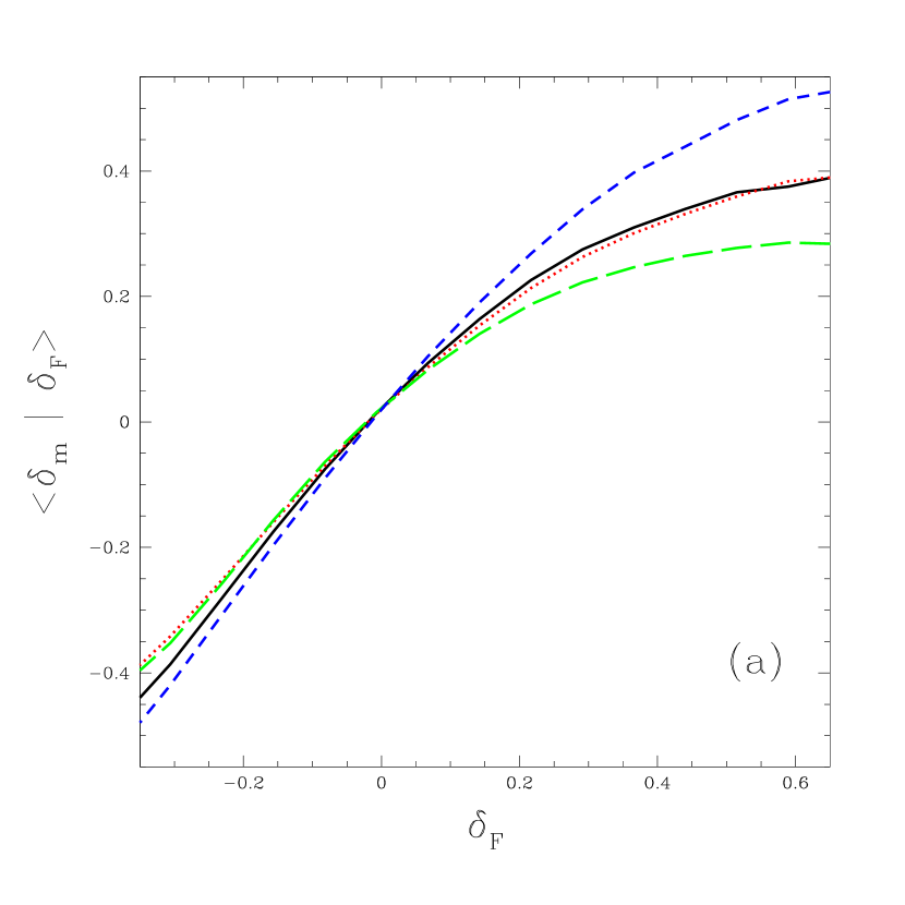
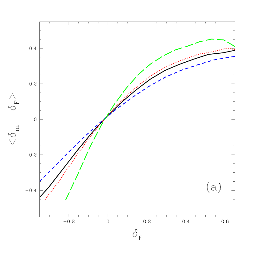
In Figure 2(a-d), we compare the results for our standard Gaussian filter (black, solid line) to the results obtained if we simply average the Ly$\alpha$ forest flux across the $10\,h^{-1}\,{\rm Mpc}$ extent of the cube with which the mass is smoothed, i.e., use a top-hat filter with $R=5\,h^{-1}\,{\rm Mpc}$ (red, dotted line). The difference is not large, although noticeable, for the $\delta_{m}$-$\delta_{F}$ relations, and is practically zero for the $\tilde{\delta}_{m}$-$\tilde{\delta}_{F}$ relations.

We also show in Figure 2 the effect of changing the size of the cube used to smooth the mass density field from $10\,h^{-1}\,{\rm Mpc}$ to $12\,h^{-1}\,{\rm Mpc}$ (green, long-dashed line) or $8\,h^{-1}\,{\rm Mpc}$ (blue, short-dashed line). In both of these cases we also change the smoothing length for the spectrum by the same factor. As the size of the smoothing cube is reduced, the mass fluctuations increase and they are more strongly correlated with the Ly$\alpha$ forest, as expected. We see that for $<\!\delta_{m}|\delta_{F}\!>$ it is important to match the dimensions of the cube in the simulations and observations to compare the two. Note, however, that the transverse angular size of the cube depends on the cosmological geometry. The other plots show less sensitivity to the cube size.

To promote comparison between our results and observations or other simulations, in Table 1 we give $<\!\tilde{\delta}_{m}|\tilde{\delta}_{F}\!>$ and $<\!\tilde{\delta}_{F}|\tilde{\delta}_{m}\!>$ for the three cube sizes, along with $\sigma_{F}$ and $\sigma_{m}$ needed to convert from $\tilde{\delta}$ to $\delta$. The rows in the Table labeled 2s, 2ld, and 2sd correspond to cube size $10\,h^{-1}\,{\rm Mpc}$, $12\,h^{-1}\,{\rm Mpc}$, and $8\,h^{-1}\,{\rm Mpc}$, respectively.

2.3 Test of the HPM Approximation

We resort to approximate HPM simulations (Gnedin & Hui 1998) because it is impractical at the present time to perform fully hydrodynamic simulations of the required size for all of the parameter variations we would like to explore. However, we first test the accuracy of the HPM approximation by comparing to a state of the art hydrodynamic simulation of a similar cosmological model. This simulation is Eulerian, with box size $25\,h^{-1}\,{\rm Mpc}$ divided into $768^{3}$ cells for baryons, with $384^{3}$ dark matter particles (see Cen et al. 2001 for a more complete description). We compare to a $25\,h^{-1}\,{\rm Mpc}$, $512^{3}$ particle HPM simulation with identical initial Fourier modes up to the Nyquist frequency of the mesh (as we show in the next subsection, the resolution of these simulations is sufficient for convergence of our chosen statistics, so we do not need to worry about exactly how to equate resolution between the two).

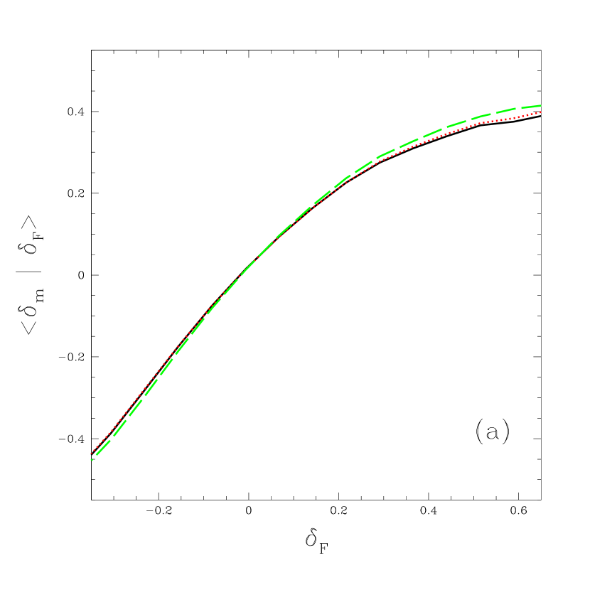
The comparison for our statistics is shown in Figure 3, where the solid lines are the HPM results and the dotted lines are the fully hydrodynamic results.

Figure 3: Test of the HPM approximation. Black (solid) lines: HPM results; red (dotted) lines: fully hydrodynamic results; green (dashed) lines: PDF of $\delta_{F}$ (a) and $\delta_{m}$ (b). The normalization of the PDFs is arbitrary.

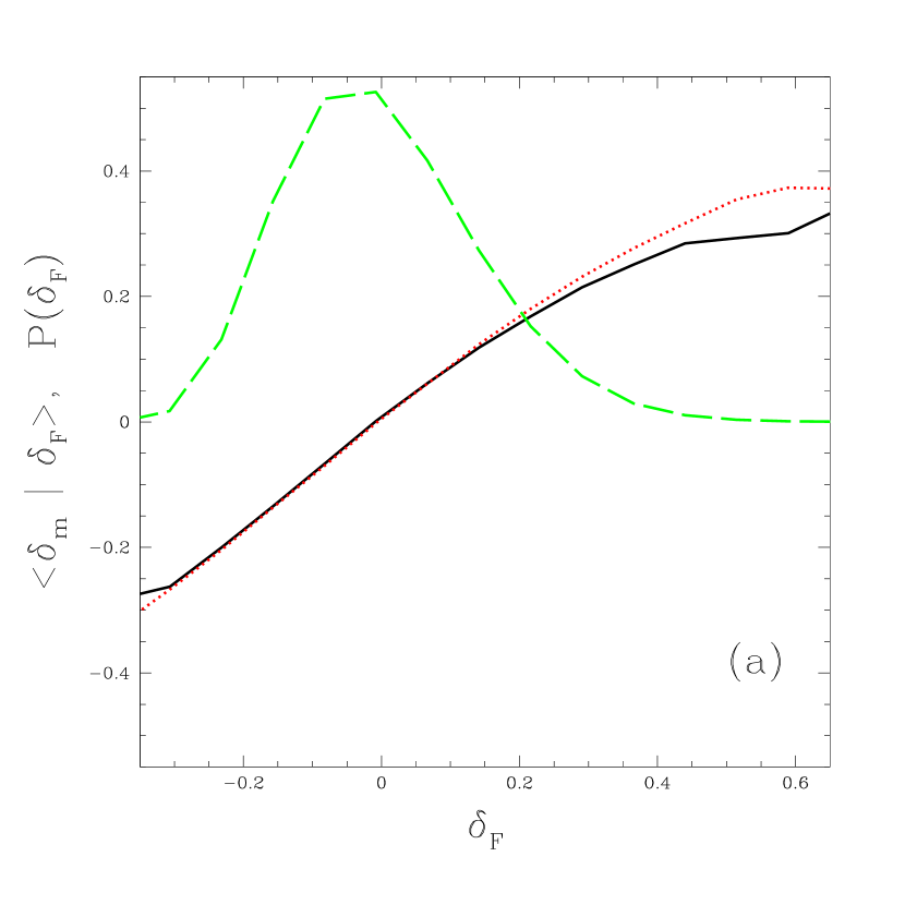
The agreement is excellent except in the highest $\delta_{F}$ regions in the $<\!\delta_{m}|\delta_{F}\!>$ and $<\!\tilde{\delta}_{m}|\tilde{\delta}_{F}\!>$ comparisons (a and c). For reference, in Figure 3(a and b) we plot the PDFs of $\delta_{F}$ and $\delta_{m}$, respectively (defined as the relative volume-weighted probability of finding $\delta$ within each of our usual bins). We see that the regions where the HPM approximation breaks down are extremely rare (at low $\delta_{m}$ in Figure 2b the lines terminate at the lowest density found in the simulations).

2.4 Convergence of the Results with Resolution and Box Size

We start by testing the sensitivity of our numerical results to the resolution. For this purpose, we use boxes with size $20\,h^{-1}\,{\rm Mpc}$ in addition to our standard value of $40\,h^{-1}\,{\rm Mpc}$.

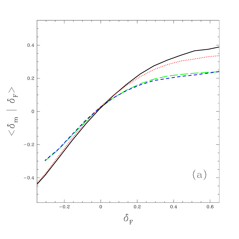
The results for the four functions, $<\!\delta_{m}|\delta_{F}\!>$, $<\!\delta_{F}|\delta_{m}\!>$, $<\!\tilde{\delta}_{m}|\tilde{\delta}_{F}\!>$, and $<\!\tilde{\delta}_{F}|\tilde{\delta}_{m}\!>$, are shown in Figures 4(a,b,c,d) for our standard cosmological model, with box size $20\,h^{-1}\,{\rm Mpc}$, and resolution of $512^{3}$ and $256^{3}$ particles for the long-dashed and short-dashed lines, respectively. The solid and dotted lines show results with box size $40\,h^{-1}\,{\rm Mpc}$, again with $512^{3}$ and $256^{3}$ particles, respectively.

Figure 4: Resolution tests. Green (long-dashed) line: $20\,h^{-1}\,{\rm Mpc}$ simulation box with $512^{3}$ particles; blue (short-dashed) line: $20\,h^{-1}\,{\rm Mpc}$, $256^{3}$ particles. Black (solid) line: $40\,h^{-1}\,{\rm Mpc}$, $512^{3}$ particles; red (dotted) line: $40\,h^{-1}\,{\rm Mpc}$, $256^{3}$ particles. (a) mean mass as a function of transmitted flux, (b) mean flux as a function of mass, (c and d) are as (a and b) except that $\delta_{F}$ and $\delta_{m}$ are divided by their rms fluctuation. The mass is always computed in redshift space.

The agreement between the $20\,h^{-1}\,{\rm Mpc}$ simulations differing only in the resolution is excellent, verifying that $40\,h^{-1}\,{\rm Mpc}$ simulations with $512^{3}$ particles should be well resolved. The agreement between $40\,h^{-1}\,{\rm Mpc}$ simulations with different resolution is still quite good except at high $\delta_{F}$, indicating that $80\,h^{-1}\,{\rm Mpc}$, $512^{3}$ particle simulations could still be useful.

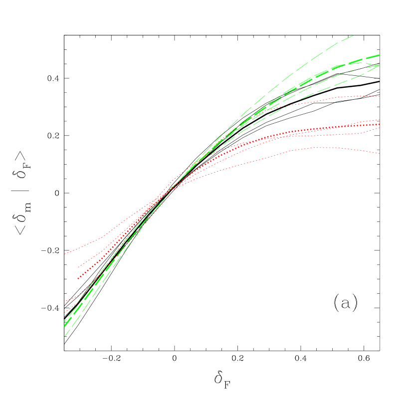
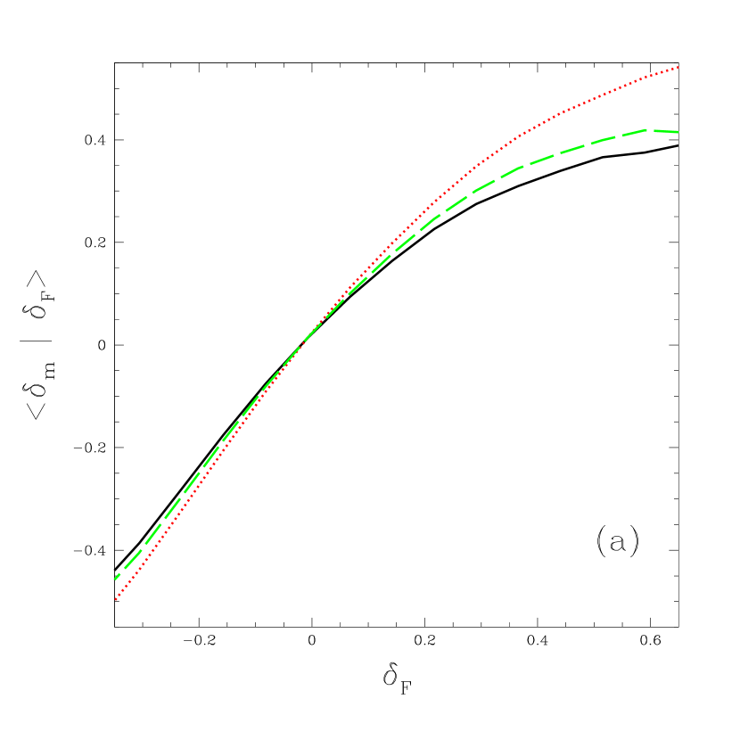
Figure 4 shows a disturbingly large difference between the results for $20\,h^{-1}\,{\rm Mpc}$ and $40\,h^{-1}\,{\rm Mpc}$ boxes; however, assessing the effect of the box size is more difficult than for the resolution, because we cannot use the same set of initial mode amplitudes at each wavenumber, so the statistical fluctuations in the simulations introduce significant random differences in the result. Figures 5(a-d) compare results for $40\,h^{-1}\,{\rm Mpc}$ boxes (black, solid lines), $20\,h^{-1}\,{\rm Mpc}$ boxes (red, dotted lines), and $80\,h^{-1}\,{\rm Mpc}$ boxes (green, dashed lines), all with $512^{3}$ particles.

Figure 5: Box size and statistical error test. The thin curves are from four independent simulations, the thick curves are the average of the four. Black (solid) lines: $40\,h^{-1}\,{\rm Mpc}$ simulations; red (dotted) lines: $20\,h^{-1}\,{\rm Mpc}$ simulations; green (dashed) lines: $80\,h^{-1}\,{\rm Mpc}$ simulations. All with $512^{3}$ particles (the $80\,h^{-1}\,{\rm Mpc}$ simulations are slightly under-resolved).

The thick lines show the average of four simulations, and the thin lines show the results from each separate simulation to demonstrate the statistical error in the curves.

Figure 5(a) shows good agreement between the 40 and $80\,h^{-1}\,{\rm Mpc}$ boxes for $<\!\delta_{m}|\delta_{F}\!>$, except at large $\delta_{F}$, where the trend toward increasing mean mass with increasing box size from 20 to 40 to $80\,h^{-1}\,{\rm Mpc}$ is probably not a result of statistical fluctuations. In fact, the true difference between the 40 and $80\,h^{-1}\,{\rm Mpc}$ boxes is even larger than what is shown because the decreased resolution in the $80\,h^{-1}\,{\rm Mpc}$ box has the effect of suppressing $<\!\delta_{m}|\delta_{F}\!>$ at large $\delta_{F}$ (see Figure 4a). It is clear that much of the flattening of $<\!\delta_{m}|\delta_{F}\!>$ that we see at large $\delta_{F}$ is an effect of the finite box size. Fortunately, the other statistics shown in Figure 5(b-d) generally exhibit better convergence than $<\!\delta_{m}|\delta_{F}\!>$.

The results in Figures 5(a-d) should also serve as a cautionary reminder that statistical fluctuations from one simulation to another can be large, and must be taken into account when comparing to observations or to other simulations, especially single, relatively small simulations. Surprisingly, the scatter between the separate simulations in the high $\delta_{F}$ corner of the plot is not reduced by increasing the box size from 40 to $80\,h^{-1}\,{\rm Mpc}$. This may be an indication that the statistical fluctuations in the result are still dominated by the longest wavelength modes in the box.

For reference, for our standard model, in a $40\,h^{-1}\,{\rm Mpc}$ box with our standard smoothing, the rms fluctuations in $\delta_{F}$ and $\delta_{m}$ are $\sigma_{F}=0.16$ and $\sigma_{m}=0.30$.

3 PARAMETER DEPENDENCE OF THE LY$\alpha$ FOREST - MASS CORRELATION

We now examine the dependence of the four functions $<\!\delta_{m}|\delta_{F}\!>$, $<\!\delta_{F}|\delta_{m}\!>$, $<\!\tilde{\delta}_{m}|\tilde{\delta}_{F}\!>$, and $<\!\tilde{\delta}_{F}|\tilde{\delta}_{m}\!>$ on the most important parameters determining the properties of the Ly$\alpha$ forest. These are the mean transmitted flux, the mean temperature-density relation of the intergalactic gas (parameterized as $T=T_{0}\Delta^{\gamma-1}$), and the amplitude and power-law slope of the power spectrum. These parameters fully determine all the physical effects that are incorporated in an HPM simulation and the calculation of the Ly$\alpha$ spectra: the underlying dark matter fluctuations (assumed to be Gaussian initially), the smoothing of the gas distribution on the Jeans scale, and the neutral fraction of the gas and thermal broadening.

3.1 Mean transmitted flux

The value of the mean transmitted flux used in our standard model, $\bar{F}=0.67$, is appropriate for $z=3$. The variation of the mean transmitted flux is the most important factor accounting for the changes in the Ly$\alpha$ forest with redshift.

Figures 6(a-d) show the four functions defined previously for $\bar{F}=0.67$ (black, solid line), $\bar{F}=0.8$, appropriate for $z\simeq 2.5$ (green, long-dashed line), $\bar{F}=0.6$, appropriate for $z\simeq 3.5$ (blue, short-dashed line), and $\bar{F}=0.7$ (red, dotted line).

Figure 6: Effect of mean transmitted flux fraction. Shown are $\bar{F}=0.67$ (black, solid line), $\bar{F}=0.8$, (green, long-dashed line), $\bar{F}=0.6$, (blue, short-dashed line), and $\bar{F}=0.7$ (red, dotted line), for the same four functions as previously.

The functions $<\!\delta_{m}|\delta_{F}\!>$ and $<\!\delta_{F}|\delta_{m}\!>$ depend strongly on $\bar{F}$, whereas the functions with the normalized quantities $<\!\tilde{\delta}_{m}|\tilde{\delta}_{F}\!>$ and $<\!\tilde{\delta}_{F}|\tilde{\delta}_{m}\!>$ have a much weaker dependence. Essentially, the mean transmitted flux changes the effective “bias” in the Ly$\alpha$ forest that determines the value of $\delta_{F}$ that corresponds to a given mass fluctuation, and once a linear bias is eliminated the dependence on $\bar{F}$ is much smaller. Note that Figures 6a,b reflect the fact that the Ly$\alpha$ forest bias is larger for higher mean flux decrements (see Figure 10c of McDonald 2002, and Croft et al. 1999, McDonald et al. 2000).

We give the results for $\bar{F}=0.6$ and $\bar{F}=0.8$ in Table 1, as rows 6sd and 6ld, respectively. The first row in the Table already contains the results for $\bar{F}=0.67$.

3.2 Temperature-density relation

The temperature-density relation has practically no effect on the functions we are analyzing, as shown in Figures 7(a-d).

Figure 7: Effect of temperature-density relation. Black, solid line: $T_{1.4}=17000$ K, $\gamma-1=0.3$ (standard values); red, dotted line: $T_{1.4}=22000$ K, $\gamma-1=0.3$; green, dashed line: $T_{1.4}=17000$ K, $\gamma-1=0.6$.

The reason for this insensitivity is that the temperature-density relation does not affect the large-scale properties of the Ly$\alpha$ forest directly, and apparently its effect through the large-scale bias factor is quite small (see Figure 10b in McDonald 2002).

3.3 Amplitude of the power spectrum

In Figure 8, we show the variations with the amplitude of the mass power spectrum by increasing the amplitude in our standard model, shown by the solid line, by 33%, to produce the dotted line. In practice, we do this by simply using an output of the same simulation at a scale factor $1.33$ times larger, but keeping the mean transmitted flux in the Ly$\alpha$ spectrum constant (this is completely equivalent to running a new simulation with a different amplitude, except that the effective temperature changes due to the change in the relation between comoving distance and velocity, but the previous figures show that the temperature does not affect the results).

Figure 8: Effect of the mass power spectrum. Black, solid line: Standard power spectrum. Red, dotted line: rms amplitude increased by 33%. Green, dashed line: $n=0.85$ instead of $n=0.95$, with fixed amplitude at $k=1~{}(\,h^{-1}\,{\rm Mpc})^{-1}$.

The result reflects that the bias factor of the Ly$\alpha$ forest decreases with increasing power spectrum amplitude (see Figure 10a of McDonald 2002). The difference is partially cancelled when using the normalized variables $\tilde{\delta}_{F}$ and $\tilde{\delta}_{m}$, although less so for the function $<\tilde{\delta}_{F}|\tilde{\delta}_{m}>$.

We also vary the power-law slope of the power spectrum in Figure 8, by changing $n$ from 0.95 to 0.85 while holding the power fixed at wavenumber $k=1\,h^{-1}\,{\rm Mpc}$. The effect we see is relatively small. Had we carefully chosen the value of $k$ at which we hold the power fixed to minimize the variation with $n$, the effect might be even smaller.

We give the results for $\sigma_{8}=1$ and $n=0.85$ in Table 1, as rows 8d and 8ld, respectively. The first row in the Table is for the standard power spectrum.

4 DISCUSSION

We have presented predictions for the expected correlation of the mass and the Ly$\alpha$ forest transmitted flux, smoothed over a cube size of $\sim 10\,h^{-1}\,{\rm Mpc}$. Our most basic result is that the relation between $<\!\tilde{\delta}_{m}|\tilde{\delta}_{F}\!>$ and $\tilde{\delta}_{F}$ is linear over most of the range of $\tilde{\delta}_{F}$ (excluding rare, high $\tilde{\delta}_{F}$ values), with a slope of 0.6 on this smoothing scale. We have shown that this correlation is not sensitive to the temperature-density relation of the gas. There is a dependence on the mean transmitted flux and the amplitude of the mass power spectrum, but these quantities are already measured to reasonable accuracy (Croft et al. 1999, McDonald et al. 2000). We have also shown that the predictions do not suffer from uncertainties due to the resolution of the simulations. Calculations with even larger boxes than used here will be desirable, because the uncertainties in the predictions due to the variance in the simulations and the suppression of the large-scale power may still be significant; however, this uncertainty is mostly isolated in the most rare, high density regions.

A similar relation holds between $<\!\tilde{\delta}_{F}|\tilde{\delta}_{m}\!>$ and $\tilde{\delta}_{m}$. We notice, however, that the observational determination of this other function will be affected by galaxy shot noise. The number of galaxies observed in a certain cube in redshift space containing a fixed mass is subject to shot noise, and this inevitably introduces a smoothing of the function $<\!\tilde{\delta}_{F}|\tilde{\delta}_{m}\!>$, which must be taken into account before any comparisons to our theoretical results are made (in contrast, galaxy shot noise does not change the average $<\!\delta_{F}|\delta_{m}\!>$, but it does alter the rms dispersion $\sigma_{F}$ needed to compute $\tilde{\delta}_{F}$). Measuring the effects of galaxy shot noise can also teach us useful information about how galaxies form, because galaxy shot noise does not generally need to be strictly described by Poisson statistics. For example, for a fixed mass contained within a cube, once a galaxy is found in the cube the probability to find others may be lower because some mass has already been used up by that galaxy.

Comparing these theoretical predictions with observations allows for several tests of the basic theory of the Ly$\alpha$ forest, and can reveal new information on the spatial distribution of the galaxies. The functions $<\!\tilde{\delta}_{m}|\tilde{\delta}_{F}\!>$ and $<\!\tilde{\delta}_{F}|\tilde{\delta}_{m}\!>$, which should not be affected by any linear galaxy bias, provide a powerful test of the assumption that the basic framework assumed here for the nature of the Ly$\alpha$ forest is correct, and that galaxies trace the mass on large scales apart from linear bias. If the slope of $<\!\tilde{\delta}_{m}|\tilde{\delta}_{F}\!>$ as a function of $\tilde{\delta}_{F}$ were found to be larger than predicted, this would imply that the Ly$\alpha$ forest is much more closely associated with galaxies than is expected from their common correlation with the mass distribution. If the observed slope were smaller than predicted, it would indicate that the Ly$\alpha$ absorbing gas and the galaxies tend to avoid each other for some reason.

If the correlation of $\tilde{\delta}_{m}$ and $\tilde{\delta}_{F}$ is as expected, this will imply a strong confirmation of the basic model we have for the Ly$\alpha$ forest, and will justify using the Ly$\alpha$ forest as a predictor of the mass fluctuations. Comparing the predicted function $<\!\delta_{m}|\delta_{F}\!>$ with the observed $<\!\delta_{g}|\delta_{F}\!>$ will then yield the bias factor of any type of galaxies for which these observations can be made.

The correlation of galaxies and the Ly$\alpha$ forest can be measured as a function of scale. Our predicted value of 0.6 for the slope of $<\!\tilde{\delta}_{m}|\tilde{\delta}_{F}\!>$ as a function of $\tilde{\delta}_{F}$ should decrease with the smoothing scale, in a way that reflects the shape of the mass autocorrelation function. This will allow a precise test of the idea that the large-scale distributions of different types of galaxies differ only in a constant linear bias relative to the mass fluctuations.

Table 1: Selected Results

Fig.,			$<\tilde{\delta}_{m}|\tilde{\delta}_{F}>$				$<\tilde{\delta}_{F}|\tilde{\delta}_{m}>$
line	$\sigma_{F}$	$\sigma_{m}$	$\tilde{\delta}_{F}=-1.5$	0	1.5	3	$\tilde{\delta}_{m}=-1$	0	1	2
2, s	0.16	0.30	-0.97	0.07	0.80	1.17	-0.61	0.09	0.58	1.00
2, ld	0.15	0.26	-0.95	0.09	0.73	1.03	-0.56	0.09	0.53	0.94
2, sd	0.18	0.36	-1.00	0.05	0.87	1.35	-0.68	0.12	0.63	1.05
6, ld	0.11	0.30	-1.09	0.10	0.86	1.26	-0.63	0.06	0.60	1.11
6, sd	0.19	0.30	-0.92	0.06	0.77	1.12	-0.60	0.11	0.56	0.94
8, d	0.18	0.39	-0.98	0.06	0.84	1.27	-0.65	0.12	0.60	1.03
8, ld	0.17	0.33	-1.00	0.07	0.84	1.21	-0.64	0.11	0.60	1.03

Note. — First column gives the Figure and curve to which the row of results applies. Solid line=s, dotted=d, long-dashed=ld, and short-dashed=sd. Value for $<\tilde{\delta}_{m}|\tilde{\delta}_{F}=3>$ underestimated due to limited box size. $\sigma_{m}$ and $\sigma_{F}$ intended only for use as conversion factors from $\tilde{\delta}$ to $\delta$ – alone they may be sensitive to resolution and box size.