Generalizing the MOND description of rotation curves

Abstract

We present new mathematical alternatives for explaining rotation curves of spiral galaxies in the MOND context. For given total masses, it is shown that various mathematical alternatives to MOND, while predicting flat rotation curves for large radii ($r/r_{d}\gg 4$, where $r_{d}$ is the characteristic radius of the galactic disc), predict curves with different peculiar features for smaller radii ($0.1<r/r_{d}\lesssim 4$). They are thus testable against observational data.

,

1 Introduction

The first mathematical descriptions of the effects of gravity, made by Galileo in his study of the free fall of bodies and by Kepler in his study of planetary motions, were purely empirical. Though Newton offered a coherent explanation of what was behind the laws governing gravitational effects, it was only with Einstein’s General Relativity that we had an apparently complete theory of gravity.

However, at the end of the 20^th century, a new enigma concerning the motion of ‘celestial bodies’ emerged, in particular, in studying rotation curves of spiral galaxies. While Newton’s law of gravity predicts that the velocity of rotation in the interior of a galaxy should fall with increasing distance from the galactic center if the observed light traces mass, what is observed is the maintenance of a constant velocity with increasing radius, generating flat rotation curves [1].

Two simple ways of dealing with this problem have been suggested:

1. assuming that there is more mass (i.e., dark matter) in galaxies than is observed;

2. modifying the law of gravity.

While much work has been done in the search for possible particle candidates for dark matter [2], very little has been done to explore the possibilities of modified gravity laws. Until now, the most popular suggestion for a modified gravitational law has been Modified Newtonian Dynamics, or, MOND [3, 4, 5]. In MOND the acceleration $a$ of a body in an external gravitational field is not exactly equal to the acceleration $g_{N}$ obtained from the Newtonian gravitational force. Mathematically, one can write $a\mu=g_{N}$, where $\mu\left(x\right)$ is a dimensionless function of the ratio $x\equiv a/a_{0}$ of the acceleration $a$ to an empirically determined constant $a_{0}$. Only in the limit $a\gg a_{0}$ is Newtonian gravity restored. The strongest objection to MOND is that it does not have a relativistic theory supporting it. For recent articles criticizing MOND, see Scott et al. (2001) [6] and Aguirre et al. (2001) [7]. For a recent positive review of MOND, see Sanders (2001) [8].

The objective of this letter is to expand the original MOND proposal by presenting mathematical alternatives for the modified gravitational law. Specifically, we present several alternative mathematical alternative formulations for the dimensionless function $\mu$, thus following closer the structure of the pioneering work of MOND by Milgrom [3, 4, 5]. In the next section we present the basics of MOND. Simulated rotation curves for several possible MONDian-like functions are given in Section 3. The final section presents some brief conclusions and perspectives for future work.

2 MOND

As discussed in the introduction, the original MOND proposal uses the relation

$$a\mu=g_{N}\;\;,$$ (1)

where $g_{N}$ is the usual Newtonian acceleration and $\mu\left(x\right)$ is a function which obeys

$$\mu\left(x\right)=\left\{\begin{array}[]{lll}1&&\left(x\gg 1\right)\\ x&&\left(x\ll 1\right)\end{array}\right.\;\;.$$ (2)

Therefore, in the limit of large accelerations, $x\gg 1$, the usual Newtonian gravity law is obtained. In the other extreme, $x\ll 1$, however, we have

$$a\mu\simeq a^{2}/a_{0}=g_{N}=GMr^{-2}\;\;.$$ (3)

Thus, using $a=V^{2}r^{-1}$, where $V$ is the rotation velocity of the galaxy,

$$V\simeq\left(GMa_{0}\right)^{1/4}\;\;,$$ (4)

which is a constant, as is observed for large galactic radii.

It is common in the literature (e.g. [6], [7]) to use the expression

$$\mu\left(x\right)=x\left(1+x^{2}\right)^{-1/2}\;\;.$$ (5)

This formula, proposed by Milgrom [3, 4, 5], has the advantage of being invertible. With it one can solve eq. (1) analytically for the acceleration $a$ and, consequently, for the rotation velocity $V$ as a function of the radius $r$. However, other functions are also possible, and are discussed in the next section.

3 Alternative mathematical formulations of MOND

In his work on the implications of MOND for galaxies [4], Milgrom used as a model for a spiral galaxy of total mass $M$, a disc of mass $M_{d}$ and a central spheroidal bulge of mass $M_{s}$. The fractional masses for the disc and the spherical bulge are $\alpha_{d}\equiv M_{d}/M$ and $\alpha_{s}\equiv M_{s}/M=1-\alpha_{d}$, respectively, so that the total fractional mass $\gamma\equiv M\left(r\right)/M$ inside a radius $r\equiv sr_{d}$ is

$$\gamma\left(s\right)=\alpha_{d}\gamma_{d}\left(s\right)+\left(1-\alpha_{d}\right)\gamma_{s}\left(s\right)\;\;,$$ (6)

where [4]

$$\gamma_{d}\left(s\right)=\left(\frac{s^{3}}{2}\right)\left[I_{0}\left(\frac{s}{2}\right)K_{0}\left(\frac{s}{2}\right)-I_{1}\left(\frac{s}{2}\right)K_{1}\left(\frac{s}{2}\right)\right]\;,$$ (7)

$$\gamma_{s}\left(s\right)=\frac{\sqrt{8\pi^{3}}b^{-9}}{m_{t}}\gamma\left(8.5,bs^{1/4}u^{-1/4}\right)\;\;,$$ (8)

and $\gamma\left(a,z\right)=\int_{0}^{z}e^{-t}t^{a-1}dt$ is the incomplete gamma function. $b=7.66924944$ and $m_{t}=2.4082\times 10^{-3}$ are numerical constants. The dimensionless variable $s=r/r_{d}=ur/r_{s}$ is the ratio of the radius $r$ to the characteristic length $r_{d}$. The ratio of $r_{s}$ to $r_{d}$, $u=r_{s}/r_{d}$, is less than unity. The radii $r_{d}$ and $r_{s}$ are obtained, in practice, by adjusting the luminosity profiles of the spheroidal and disc components, using the empirical law of de Vaucoulers for the spherical bulge and an exponential function for the disc.

Following the MOND proposal, we define

$$a=\mu^{\prime}\left(y\right)g_{N}\;,$$ (9)

where $\mu^{\prime}$ is a dimensionless function with a dimensionless argument $y\equiv r\sqrt{a_{0}G^{-1}M^{-1}(r)}$, similar to the $\mu$ of Milgrom [3, 4, 5] in eq. (5). This new function $\mu^{\prime}\left(y\right)$ is such that

$$\mu^{\prime}\left(y\right)=\left\{\begin{array}[]{lll}y&&\left(y\gg 1\right)\\ 1&&\left(y\ll 1\right)\end{array}\right.\;\;.$$ (10)

We investigate the following functions $\mu^{\prime}\left(y\right)$ which obey the constraints of eq. (10):

$$\left\{\begin{array}[]{l}\mu^{\prime}_{1}=\sqrt{1+y^{2}}\\ \mu^{\prime}_{2}=y\coth y\\ \mu^{\prime}_{3}=y\left(1-e^{-y}\right)^{-1}\\ \mu^{\prime}_{4}=y\left(\coth 3y-\frac{1}{3y}\right)^{-1}\end{array}\right.\;\;.$$ (11)

The behaviour of each of these functions as a function of $y$ can be seen in the expansions [9]

$$\left\{\begin{array}[]{l}\begin{array}[]{ll}\mu_{1}^{\prime}&=\sum_{k=0}^{\infty}\Gamma\left(n-1/2\right)\left(2\sqrt{\pi}n!\right)^{-1}(-1)^{n-1}y^{2n}\\ &=1+y^{2}/2-y^{4}/8+y^{4}/16-5y^{6}/128+...\end{array}\\ \begin{array}[]{llr}\mu_{2}^{\prime}&=1+2y^{2}\sum_{k=1}^{\infty}\left(y^{2}+k^{2}\pi^{2}\right)^{-1}&\\ &\simeq 1+y^{2}/3-y^{4}/45+2y^{6}/245+...&\left(y<\pi\right)\end{array}\\ \begin{array}[]{llr}\mu_{3}^{\prime}&=y\sum_{k=0}^{\infty}e^{-ky}&\\ &\simeq 1+y/2+y^{2}/12-y^{4}/720+y^{6}/30240+...&\left(y<2\pi\right)\end{array}\\ \begin{array}[]{llr}\mu_{4}^{\prime}&=\frac{1}{6}\left[\sum_{k=1}^{\infty}\left(9y^{2}+k^{2}\pi^{2}\right)^{-1}\right]^{-1}&\\ &\simeq 1+27y^{2}/45-\left(27y/45\right)^{4}+\left(27y/45\right)^{6}+...&\left(y\ll 1\right)\end{array}\end{array}\right.\;\;.$$ (12)

The functions are plotted in Figure 1.

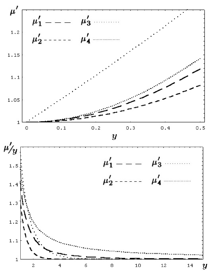
Figure 1: Top: Curves showing the behaviour of the $\mu^{\prime}$ functions as a function of $y\equiv r\sqrt{a_{0}G^{-1}M^{-1}\left(r\right)}$ for $y<1$. Bottom: Curves showing the behaviour of $\mu^{\prime}/y$ as a function of $y$ for $y>1$ (the functions $\mu_{1}^{\prime}$, $\mu_{2}^{\prime}$, $\mu_{3}^{\prime}$ and $\mu_{4}^{\prime}$ versus $y$ are defined in eq. (11)).

Using these functions, together with equations (6), (7) and (8), we obtain curves for the dimensionless rotation velocity $v\equiv V\left(r\right)/\left(GMa_{0}\right)^{1/4}$ as a function of $s=r/r_{d}$ for different values of $M$, $\alpha_{d}=M_{d}/M$, and $u=r_{s}/r_{d}$. The curves are shown in Figures 2 and 3.

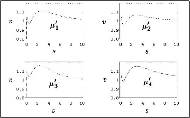
Figure 2: Curves of $v\equiv V\left(r\right)/\left(GMa_{0}\right)^{1/4}$ as a function of $s\left(=r/r_{d}\right)$ and $\mu^{\prime}$. The functions $\mu^{\prime}$ are defined in eq. (11). In all graphs, $\alpha_{d}=3/4$, $u=1/4$, and $M=M_{0}$, where $M_{0}$ is an arbitrary mass. The functions $\alpha_{d}$ and $u$ are defined as $\alpha_{d}\equiv M_{d}/M$ and $u\equiv r_{s}/r_{d}$, where $M_{d}$ is the mass of the disc and $r_{s}$ ($r_{d}$) is the effective radius of the spherical bulge (disc).

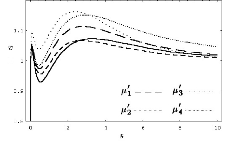
Figure 3: Curves of $v\equiv V\left(r\right)/\left(GMa_{0}\right)^{1/4}$ as a function of $s\left(=r/r_{d}\right)$ and $\mu^{\prime}$. The functions $\mu^{\prime}$ are defined in eq. (11). The solid line is the curve obtained using Milgrom’s original proposal, eq. (5). For all curves $M=M_{0}$, where $M_{0}$ is an arbitrary mass, $\alpha_{d}=3/4$, $u=1/4$. The functions $\alpha_{d}$ and $u$ are defined as $\alpha_{d}\equiv M_{d}/M$ and $u\equiv r_{s}/r_{d}$, where $M_{d}$ is the mass of the disc and $r_{s}$ ($r_{d}$) is the effective radius of the spherical bulge (disc).

4 Conclusion

Inspection of Figures 2 and 3 shows clearly that all the functions $\mu^{\prime}\left(y\right)$ produce flat rotation curves. This is true not only for the particular values of $M$, $\alpha_{d}$, and $u$ of the figures, but for the entire range of physically reasonable values for these parameters. Figure 3 shows that a comparison between the curves obtained, using the different $\mu^{\prime}$ functions presented, together with the original Milgrom proposal (eq. (5)), may be useful to distinguish between them, since each curve has a peculiar feature in the region $0.1<r/r_{d}\lesssim 4$.

It would be interesting to test the formulas presented here against observational data, noting that $\alpha_{d}$ and $u$ are not free parameters, but are given by the luminosity profiles of the galaxies. The mass $M$ and the constant $a_{0}$ are the only free parameters to be adjusted. The study of different galaxies gives a single value for $a_{0}$, the mass $M$ and the mass-luminosity ratio, $M/L$, of each galaxy. $\mu$ and $\mu^{\prime}$ can lead to different relativistic extensions of MOND, important for future studies. For instance, using the expression for the gravitational potential $\varphi\left(r\right)=-\int a\left(r\right)dr$, valid for purely radial forces, one can naively ascribe a $\varphi\left(r\right)$ to the modified gravitational laws obtained with $\mu^{\prime}_{1}$, $\mu^{\prime}_{2}$ and $\mu^{\prime}_{3}$, for example,

$$\varphi_{\mu^{\prime}_{1}}\left(r\right)=-\frac{GM}{r}\sqrt{1+\frac{r^{2}a_{0}}{GM}}+\sqrt{GMa_{0}}\mathrm{arcsinh}\left(r\sqrt{\frac{a_{0}}{GM}}\right)+\varphi_{0}\;\;,$$ (13)

$$\varphi_{\mu^{\prime}_{2}}\left(r\right)=-\frac{GM}{r}+2\sqrt{GMa_{0}}\sum_{n=1}^{\infty}\frac{1}{n\pi}\arctan\left(\frac{r}{n\pi}\sqrt{\frac{a_{0}}{GM}}\right)+\varphi_{0}\;\;,$$ (14)

and

$$\varphi_{\mu^{\prime}_{3}}\left(r\right)=\sqrt{GMa_{0}}\left[\ln\left(r\sqrt{\frac{a_{0}}{GM}}\right)+\sum_{n=1}^{\infty}{\mathrm{E}i}\left(-nr\sqrt{\frac{a_{0}}{GM}}\right)\right]+\varphi_{0}\;\;,$$ (15)

where $\varphi_{0}$ is a constant of integration.

Therefore, in the search for a complete theory for MOND, it is important to study alternative MONDian functions. The MONDian functions given in this letter can be seen as a step in this direction.

References

[1] Peebles, P.J.E. – “Principles of Physical
Cosmology”, Princeton University Press, New Jersey, 1993.
[2] Khalil, S.; Muñoz, C. – e-printhep-ph 0110122 (2001).
[3] Milgrom, M. – Ap. J.270, 365 (1983).
[4] Milgrom, M. – Ap. J.270, 371 (1983).
[5] Milgrom, M. – Ap. J.270, 384 (1983).
[6] Scott, D.; White, M.; Cohn, J.D.; Pierpaoli, E. – e-printastro-ph 0104435 (2001).