Chromospherically young, kinematically old stars

We have investigated a group of stars known to have low chromospheric ages, but high kinematical ages. Isochrone, chemical and lithium ages are estimated for them. The majority of stars in this group show lithium abundances much smaller than expected for their chromospheric ages, which is interpreted as an indication of their old age. Radial velocity measurements in the literature also show that they are not close binaries. The results suggest that they can be formed from the coalescence of short-period binaries. Coalescence rates, calculated taking into account several observational data and a maximum theoretical time scale for contact, in a short-period pair, predict a number of coalesced stars similar to what we have found in the solar neighbourhood.

1 Introduction

The chromospheric activity of a late-type star is frequently interpreted as a sign of its youth. Young dwarfs show high rotation rates, and the interaction between rotation and outer envelope convection is expected to drive the chromospheric activity. Nevertheless, not only young single stars present high rotation rates. Close and contact binaries can keep high rotation over several billion years. In such stars, the rotational angular momentum loss is balanced by the proximity of the stars in the system, which results in transfer of orbital angular momentum to the rotational spins. Thus in chromospheric activity surveys aimed at late type stars, we expect to find two classes of objects: young stars and chromospherically active binaries. Sometimes, a star suspected of being young can be instead a spectroscopic binary (Soderblom et al. soder98 (1998)), not yet investigated by radial velocity surveys.

The chromospheric activity surveys by the Mount Wilson group are directed at, but not only at, late type stars. The two surveys that comprise the bulk of a sample used by some of us in the derivation of chemodynamical constraints on the evolution of the Galaxy (Rocha-Pinto et al. 2000a , 2000b ) were based on solar-type stars, in a spectral range from F8 V to K4 V. Chromospherically active binaries were generally avoided, since the surveys investigate the chromospheric activity in single stars. Due to this, the division of these surveys into two classes, of active and inactive stars, corresponds closely to an age segregation.

This was very well demonstrated by Soderblom (soder90 (1990), see also Jeffries & Jewell JJ (1993)), who studied the kinematics of active and inactive stars. The active stars are concentrated in a region of low velocities in a space velocity diagram, as expected for young objects; on the other hand, the inactive stars are scattered in this diagram, just like old stellar populations. Few active stars do not follow this rule, showing considerably high velocities. Soderblom calls attention to them, but interpret them as possible runaway stars. Rocha-Pinto et al. (paperIII (2002)) have increased the number of active stars with spatial velocities to 145. Several of these stars, show velocities which are inconsistent with their presumed age.

The term CYKOS (acronym for chromospherically young, kinematically old stars) is applied here to all chromospherically active stars which, in a velocity diagram, present velocity components greater than the expected value for such stars, irrespective of the fact that this object is an undiscovered close binary, a runaway star or another kind of object.

This paper presents several newly identified CYKOS, and proposes an explanation for some of them. It is organized as follows: in section 2, we present the sample and the method used to define a CYKOS. Section 3 analyses what is presently known about their ages from chromospheric and isochrone age measurement methods. In section 4, we show that these objects have very low Li abundances compared to other stars with the same temperature. A critical review of the literature about some individual CYKOS follow in section 5. Finally, in section 6, we propose that a small number of these objects could probably have been formed by coalescence of binaries.

Table 1: Identified CYKOS. The columns list the stellar name, MK type, $(B-V)$, chromospheric index, chromospheric and isochrone ages, heliocentric spatial velocities $U$, $V$ and $W$, and the components, according to which the object was classified as CYKOS. In the sixth cloumn, the remarks ‘ZAMS’, ‘red MS’ and ‘sd’ refer, respectively, to stars near the zero age main sequence, in the red part of the main sequence, or that are subdwarfs according to their position, and for which no age determination was possible.

HD/BD	MK	$(B-V)$	$\log R^{\prime}_{\rm HK}$	${\rm chrom.age}$	${\rm isoch.age}$	$U$	$V$	$W$	${\rm criteria}$
5303	G3: V+	$0.71$	$-4.03$	$0.38$	$2.30$	$81\pm 5$	$-58\pm 3$	$-13\pm 1$	${U}{V}\phantom{W}$
7983	G2 V	$0.59$	$-4.75$	$7.91$	$18.0$	$-138\pm 11$	$-72\pm 6$	$-51\pm 5$	${U}{V}{W}$
13445	K1 V	$0.77$	$-4.74$	$2.34$	${\rm redMS}$	$98\pm 0.7$	$-75\pm 1$	$-25\pm 2$	${U}{V}{W}$
16176	F5 V	$0.48$	$-4.73$	$2.07$	$2.0$	$25\pm 2$	$-46\pm 2$	$-22\pm 1$	$\phantom{U}{V}\phantom{W}$
20766	G2.5 V	$0.64$	$-4.65$	$2.09$	${\rm redMS}$	$71\pm 0.5$	$-47\pm 1$	$16\pm 1$	${U}{V}\phantom{W}$
39917	G8 V	$0.76$	$-4.05$	$0.28$	$1.3$	$-61\pm 6$	$-31\pm 2$	$-19\pm 2$	${U}\phantom{V}\phantom{W}$
51754	G0	$0.57$	$-4.56$	$3.35$		$-194\pm 17$	$-139\pm 13$	$3\pm 1$	${U}{V}\phantom{W}$
65721	G6 V	$0.74$	$-4.67$	$2.86$	${\rm redMS}$	$-37\pm 2$	$-39\pm 2$	$28\pm 1$	$\phantom{U}{V}\phantom{W}$
74385	K1 V	$0.91$	$-4.55$	$0.93$	${\rm redMS}$	$15\pm 0.4$	$-21\pm 2$	$-30\pm 0.5$	$\phantom{U}\phantom{V}{W}$
88742	G1 V	$0.62$	$-4.69$	$2.53$	$10.0$	$36\pm 0.5$	$-45\pm 1$	$-4\pm 1$	$\phantom{U}{V}\phantom{W}$
89995	F6 V	$0.46$	$-4.74$	$4.70$	$2.6$	$55\pm 2$	$-42\pm 2$	$-17\pm 3$	$\phantom{U}{V}\phantom{W}$
103431	dG7	$0.76$	$-4.68$	$1.74$	${\rm redMS}$	$68\pm 4$	$-39\pm 2$	$-13\pm 2$	${U}{V}\phantom{W}$
106516	F5	$0.46$	$-4.65$	$6.43$	$7.4$	$-54\pm 1$	$-74\pm 2$	$-59\pm 2$	$\phantom{U}{V}{W}$
120237	G3 IV-V	$0.58$	$-4.75$	$4.16$	$13.8$	$47\pm 2$	$-57\pm 2$	$-3\pm 1$	$\phantom{U}{V}\phantom{W}$
123651	G0/G1 V	$0.53$	$-4.74$	$5.39$	$13.0$	$29\pm 4$	$-10\pm 4$	$-33\pm 2$	$\phantom{U}\phantom{V}{W}$
131582	K3 V	$0.96$	$-4.73$	$2.79$	${\rm redMS}$	$66\pm 2$	$-67\pm 2$	$15\pm 2$	${U}{V}\phantom{W}$
131977	K4 V	$1.11$	$-4.49$	$0.21$	${\rm redMS}$	$-49\pm 2$	$-22\pm 1$	$-32\pm 1$	$\phantom{U}\phantom{V}{W}$
144872	K3 V	$0.96$	$-4.74$	$2.89$	${\rm redMS}$	$-70\pm 1$	$1\pm 1$	$-2\pm 2$	${U}\phantom{V}\phantom{W}$
149661	K2 V	$0.81$	$-4.58$	$0.83$	${\rm redMS}$	$2\pm 2$	$-1\pm 0.4$	$-30\pm 1$	$\phantom{U}\phantom{V}{W}$
152391	G8 V	$0.76$	$-4.39$	$0.28$	${\rm redMS}$	$-85\pm 2$	$-112\pm 2$	$8\pm 1$	${U}{V}\phantom{W}$
165401	G0 V	$0.63$	$-4.65$	$3.92$	$18.9$	$79\pm 2$	$-90\pm 1$	$-40\pm 1$	${U}{V}{W}$
183216	G2 V	$0.60$	$-4.62$	$0.50$	$1.8$	$40\pm 2$	$-46\pm 1$	$0\pm 1$	$\phantom{U}{V}\phantom{W}$
189931	G1 V	$0.60$	$-4.64$	$0.76$	${\rm ZAMS}$	$41\pm 2$	$-50\pm 1$	$1\pm 1$	$\phantom{U}{V}\phantom{W}$
196850	G0	$0.57$	$-4.64$	$1.31$	${\rm redMS}$	$0\pm 0.4$	$-22\pm 2$	$-33\pm 1$	$\phantom{U}\phantom{V}{W}$
209100	K4.5 V	$1.06$	$-4.56$	$0.39$	${\rm redMS}$	$80\pm 1$	$-41\pm 0.2$	$4\pm 1$	${U}{V}\phantom{W}$
219709	G2/G3 V	$0.65$	$-4.62$	$1.14$	$8.5$	$25\pm 1$	$-42\pm 1$	$-10\pm 0.1$	$\phantom{U}{V}\phantom{W}$
230409	G0	$0.70$	$-4.70$	$8.78$	${\rm sd}$	$-133\pm 16$	$-129\pm 13$	$-13\pm 1$	${U}{V}\phantom{W}$
+15 3364	G0	$0.63$	$-4.43$	$0.49$	$8.7$	$-59\pm 3$	$-22\pm 2$	$2\pm 1$	${U}\phantom{V}\phantom{W}$
+51 1696	sdG0	$0.55$	$-4.42$	$3.51$		$228\pm 23$	$-277\pm 33$	$53\pm 1$	${U}{V}{W}$

2 Identification of CYKOS

The CYKOS can be identified by a diagram of spatial velocities ($U\times V$ or $W\times V$) showing only active stars, in analogy to their first discovery by Soderblom. Not all objects identified in a $U\times V$ diagram are also identified in a $W\times V$ diagram, and vice versa. We expect that CYKOS showing high velocities in more than one component are really peculiar objects, and not just stars having a component velocity in the tail of the distribution.

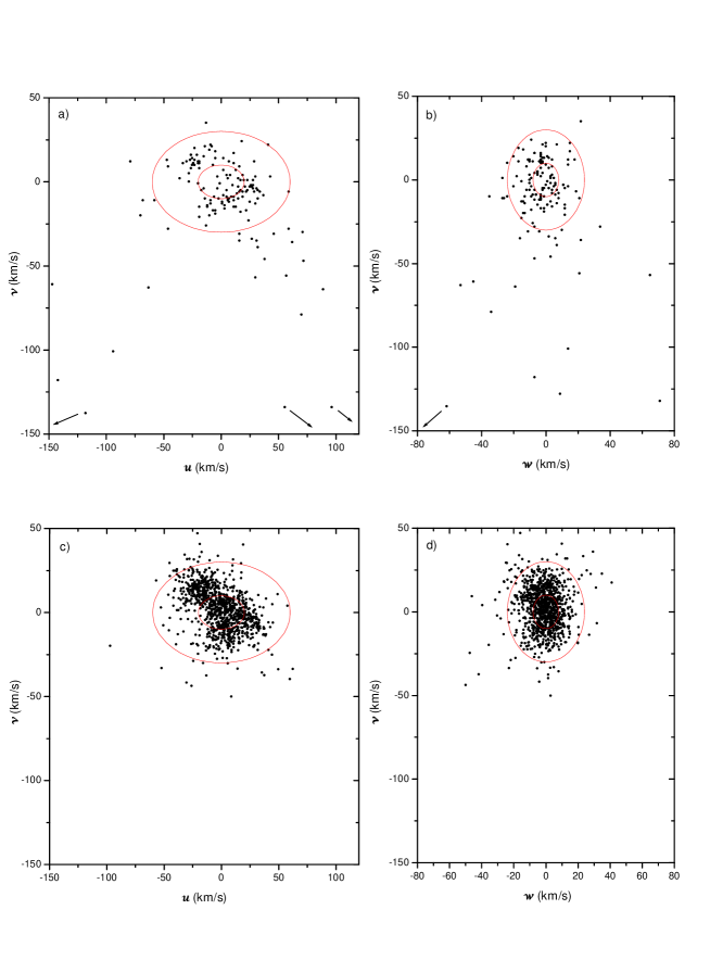
Figure 1: Panels a and b: spatial velocity diagrams for 145 active stars. The ellipses have semiaxes equal to $\sigma$ and $3\sigma$, where $\sigma$ is the velocity dispersion for stars with ages lower than 1 Gyr (Rocha-Pinto et al. paperIII (2002)) in the corresponding velocity components. For these dispersions, we use $\sigma_{u}=20$ km/s, $\sigma_{v}=10$ km/s and $\sigma_{w}=8$ km/s. Objects located beyond the outer ellipses, corresponding to $3\sigma$, are considered CYKOS. Panels c and d: spatial velocity diagrams for 1023 A dwarfs, taken from the sample of Palouš (palous (1983)). In all panels, we have used spatial velocities corrected for the solar motion (Mihalas & Binney mihalas (1981)).

Some CYKOS also appear clearly in an age–velocity diagram, so that, in principle, this diagram could also be used to identify them. However, the uncertainty in the chromospheric ages can make some inactive stars appear young in such a plot, and our main purpose is not the study of young inactive stars, but rather of active stars that are kinematically old.

We have used as our primary source the sample containing 145 active stars built by Rocha-Pinto et al. (paperIII (2002)). This sample is composed by all active stars from Rocha-Pinto et al. (2000b ) for which radial velocity measurements are available in the literature. The heliocentric velocities are calculated with the equations provided by Johnson & Soderblom (johnsod (1987)).

Figs.1a and b show the $U\times V$ and $W\times V$ diagrams for these stars. The velocities were corrected for the solar motion $(U_{\odot},V_{\odot},W_{\odot})=(-9,11,6)$ km s^-1 according to Mihalas & Binney (mihalas (1981)). In the plots, the semiaxes of the inner and outer ellipses are equal to 1$\sigma$ and 3$\sigma$, respectively, where $\sigma$ is the velocity dispersion of stars with ages lower than 1 Gyr. We have adopted $\sigma_{U}=20$ km/s, $\sigma_{V}=10$ km/s and $\sigma_{W}=8$ km/s, which correspond to the velocity dispersion of the youngest stellar population (ages 0 to 1 Gyr), according to Rocha-Pinto et al. (paperIII (2002)), and have considered as CYKOS all objects located beyond the outer ellipses. The velocity dispersions for the youngest population are in good agreement with other determinations in the literature. The values for $\sigma_{U}$ range from 11.7 km/s (Meusinger et al. meusinger (1991)) to 23 km/s (Cayrel de Strobel cayrel (1974)). The agreement is closer for $\sigma_{V}$, ranging from 5.9 km/s (Meusinger et al. meusinger (1991)) to 10.1 km/s (Cayrel de Strobel cayrel (1974)), and $\sigma_{W}$, ranging from 8 km/s (Wielen wielen (1974)) to 9.7 km/s (Cayrel de Strobel cayrel (1974)).

In Tab. (1), we list the thirty stars identified as CYKOS. The first column gives the name of the star, followed by the spectral type, $(B-V)$ colour, chromospheric activity index, chromospheric and isochrone ages, as commented upon later, and the $U$, $V$ and $W$ heliocentric velocities, which are given with formal uncertainties. The last column shows the velocity criteria used in order to classify the object as a CYKOS.

The results also show that CYKOS are generally more apparent in $V$ than in the other velocity components, as expected for a kinematically old stellar population: the $V$ component is systematically more negative than in the case of normal active stars, which are presumably young. This is an effect of the asymmetrical drift. The stars are likely to acquire increasing random velocities with respect to the local standard of rest, due to subsequent encounters with giant molecular clouds. In $U$ and $W$, there will be a symmetric increase in the velocity dispersion and we would not expect the CYKOS to be much different from the normal stars, from the consideration of these velocity components only.

The peculiar character of these objects can be seen from Figs. 1c and d, where the same diagrams are shown for 1023 A dwarfs, taken from the large compilation by Palouš (palous (1983)). Since A dwarfs are very young stars, due to their maximum life expectancy, their kinematical properties are consistent with those of very young late-type dwarfs. We do find stars having velocity components greater than 3$\sigma$, where we have used the same velocity dispersions used in Figs. 1a and b. Nevertheless, these A dwarf outliers have smaller velocities than the average velocities of the CYKOS as shown in Figs. 1a and b. Aroung 4% of the A dwarfs are outliers, while this number goes to 20% in the case of the late-type dwarfs. For the A stars, these outliers probably represent the tail of the velocity distribution, which is reinforced by the fact that their $V$ distribution is nearly symmetrical, contrary to what happens for the CYKOS.

3 What age measurement methods tell us

The chromospheric ages of half of the objects listed in Tab. (1) are lower or similar to 2 Gyr. This can be seen from the fourth and fifth columns of the Table, which give the chromospheric activity index $\log R^{\prime}_{\rm HK}$ and the chromospheric ages in Gyr, respectively. The chromospheric index was defined by Noyes et al. (annoyes (1984)) and the calculation of chromospheric ages was discussed by Rocha-Pinto & Maciel (RPM98 (1998)).

There are 9 stars in Table 1 whose chromospheric age is larger than 3 Gyr. Strictly speaking, they cannot be considered as ‘chromospherically young’, and are listed in view of their activity levels ($\log R^{\prime}_{\rm HK}>-4.75$), which traditionally indicate a young age (Soderblom soder90 (1990)). Five of them have $\log R^{\prime}_{\rm HK}\leq-4.70$. Given that the error in $\log R^{\prime}_{\rm HK}$ is expected to be around 0.04 dex, it is possible that these stars are inactive, rather than active stars. On the other hand, at least one of them presents significant X-ray emission (HD 89995). Also, we must take into account that a high chromospheric age could be caused by the metallicity of the star. Metal-poor CYKOS are also chromospherically older, due to the metallicity dependence of the chromospheric age (Rocha-Pinto & Maciel RPM98 (1998)). In fact, some of these 9 stars are metal-poor, in comparison with the majority of the other stars. However, since the metallicity introduces an additional source of error in the calculation of the chromospheric age, it is not unlikely that these objects could be younger than what is shown in Table 1. For instance, we have remarked that even some of these older CYKOS have velocities considerably larger than the mean velocity of their coeval stars (this is particularly true for the CYKOS having chromospheric age between 2 and 4 Gyr). For these reasons only, we have decided to keep them in the sample.

The basic problem deserving an explanation is why the chromospheric ages of these objects are low (sometimes very low), while their kinematic ages are high (sometimes very high). What can be said about their ages from other methods?

The objects in Tab.(1) have a broad metallicity distribution. Most of these stars have [Fe/H] between $-0.40$ and $+0.20$, but 11% of them have photometric metallicities lower than $-0.60$ dex. From the point of view of chemical evolution, they have a broad age range, with averages around 3-5 Gyr if we adopt the age–metalliticy relation given by Rocha-Pinto et al. (2000b ).

For the calculation of isochrone ages, we have used the isochrones by Bertelli et al. (bertelli (1994)). The age of the star was calculated by interpolation in each isochrone. A final interpolation, taking into account the ages at several metallicities (that is, several isochrone grids), uses the real stellar metallicity to find the stellar age. The results are shown in the sixth column of Tab. 1.

These ages are somewhat rough and some care must be taken when interpreting these results. The reason for this is that the $m_{1}$ deficiency, present in active stars (see Rocha-Pinto & Maciel RPM98 (1998), and references therein), hinders the determination of accurate stellar parameters by photometric indices. In our case, $\log T_{\rm eff}$, which is estimated from the equations given by Olsen (olsen84 (1984)), can be miscalculated. Three stars do not have parallaxes measured by HIPPARCOS, or have uvby colours outside the range covered by the calibrations by Olsen, and do not have isochrone ages in Table 1.

Nearly 40% of the stars lie in the red part of the main sequence, for which no age determination is possible. The remaining stars are distributed nearly equally between young (7 stars having less or about 2 Gyr) and old stars (8 stars with ages greater than 7 Gyr). There are no preferred ages for these stars.

Our results show that, in spite of some of CYKOS having low isochrone ages, others can be very old. The cooler stars in the red MS can have very different ages, since they are in a colour range where no perceptible evolution in the HR diagram is visible.

4 Lithium in CYKOS

Table 2: Observations of CYKOS and active stars.

HD/BD	R.A. (2000)			Dec. (2000)			J.D.	exp.	Teff	$\log g$	$\xi_{T}$	${\rm[Fe/H]}$	N(Li)	vr
	h	m	s	$\degr$	′	′′	(2451000 +)	(s)	(K)		(km/s)			(km/s)
870	00	12	51	$-$57	54	48	037.782	900	5350	4.40	0.5	$-0.12$	0.50	$-$2
1237	00	16	04	$-$79	51	02	384.785	660	5250	4.33	0.7	$0.00$	1.90	$-$3
13445	02	10	15	$-$50	50	00	037.836	900	5270	4.50	0.8	$-0.10$	0.50	+53
17051	02	42	31	$-$50	48	12	384.837	450	6040	4.25	1.0	$0.10$	2.40	+4
20766	03	17	36	$-$62	35	04	037.850	600	5715	4.30	1.0	$-0.20$	0.50	+9
22049	03	32	59	$-$09	27	31	384.832	220	5215	4.83	1.3	$-0.15$	0.75
106516	12	15	10	$-$10	17	54	384.398	600	6190	4.20	1.0	$-0.55$	$<1.20$	+8
124580	14	15	38	$-$44	59	55	037.410	1200	5845	4.28	1.5	$-0.20$	2.75	+4
131977	14	54	32	$-$21	11	28	033.452	900	4585	4.58	1.0	$0.20$	$<-1.00$	+26
138268	14	15	58	$-$44	59	55	033.502	2400	5975	4.40	1.0	$0.30$	2.90	$-$59
”							037.426	1200					2.90
149661	16	36	19	$-$02	19	13	037.442	600	5235	4.50	1.0	$0.05$	$<-1.00$	$-$14
152391	16	53	01	$-$00	00	22	037.455	900	5450	4.37	1.2	$0.00$	1.10	+44
154417	17	05	16	00	42	25	037.481	666	5970	4.35	1.3	$-0.10$	2.80	$-$18
165401	18	05	37	04	39	42	037.468	900	5755	4.21	1.0	$-0.40$	0.50	$-$120
174429	18	53	05	$-$50	10	49	037.528	1320	5100	4.10			3.00	$-$10
181321	19	21	29	$-$34	58	56	037.567	780	5975	4.30	1.5	$0.10$	3.10	$-$19
185124	19	37	46	$-$04	38	48	037.579	480	6760	4.20			2.80	$-$33
189931	20	04	02	$-$37	52	15	037.587	900	5865	4.35	1.0	$0.10$	2.15	$-$44
202628	21	18	25	$-$43	20	05	384.697	660	5750	4.24	1.0	$0.05$	2.15	+9
202917	21	20	49	$-$53	01	58	384.672	1800	5555	4.25	1.6	$0.05$	3.35	$-$1
206667	21	44	44	$-$42	07	46	384.709	1000	5950	4.22	1.0	$0.00$	2.40	+14
209100	22	03	21	$-$56	47	09	384.664	400	4660	4.90	1.5	$0.10$	0.15	$-$44
217343	23	00	18	$-$26	09	05	384.723	900	5755	4.44	1.3	$0.00$	3.20	$-$9
221231	23	31	00	$-$69	04	29	384.751	800	5910	4.42	1.3	$0.00$	2.95	+2
223913	23	53	40	$-$65	56	55	384.762	660	5985	4.50	1.0	$0.15$	2.65	+18
+15 3364	18	07	18	15	56	54	037.491	1800	5685	4.20	0.8	$0.00$	0.00	+24
”							037.504	1800					0.00

Although Li depletion and production in stars are processes not completely well understood, in some cases the Li abundance could be used as a youth indicator. If CYKOS are young objects, as suggested by their chromospheric activity, they must present high Li abundances. On the other hand, if they show very depleted Li, they must be evolved objects, irrespective of what their magnetic activity might tell us.

4.1 Observations

We have obtained spectra for 28 stars, including CYKOS and normal active stars (used as reference objects). The observations were carried out at the Laboratório Nacional de Astrofísica (LNA, Brazil) in two observing runs, in August 1998 and July 1999. The spectra were obtained with the coudé spectrograph at the 1.6m telescope, using a SITe CCD of 1024$\times$1024 pixels with 24$\mu$m$\times$24$\mu$m pixel size, and a grating of 1800 l/mm yielding a resolution over two pixels of $\approx$ 24,000 covering the wavelength range $\lambda\lambda$ 6640–6780 Å.

The data were reduced using standard tasks of IRAF package. Spectra from different exposures were added by weighting them with (S/N)². The final S/N ratio for the stars are in the range of 100 to 200. The spectrum of a hot star obtained with the same configuration was inspected for telluric lines. The log of observations is reported in Table 2 together with some other information. The radial velocities listed were calculated using a set of unblended atomic lines in the same data. The error in the radial velocity is 2 km/s.

4.2 Spectra of normal stars and CYKOS

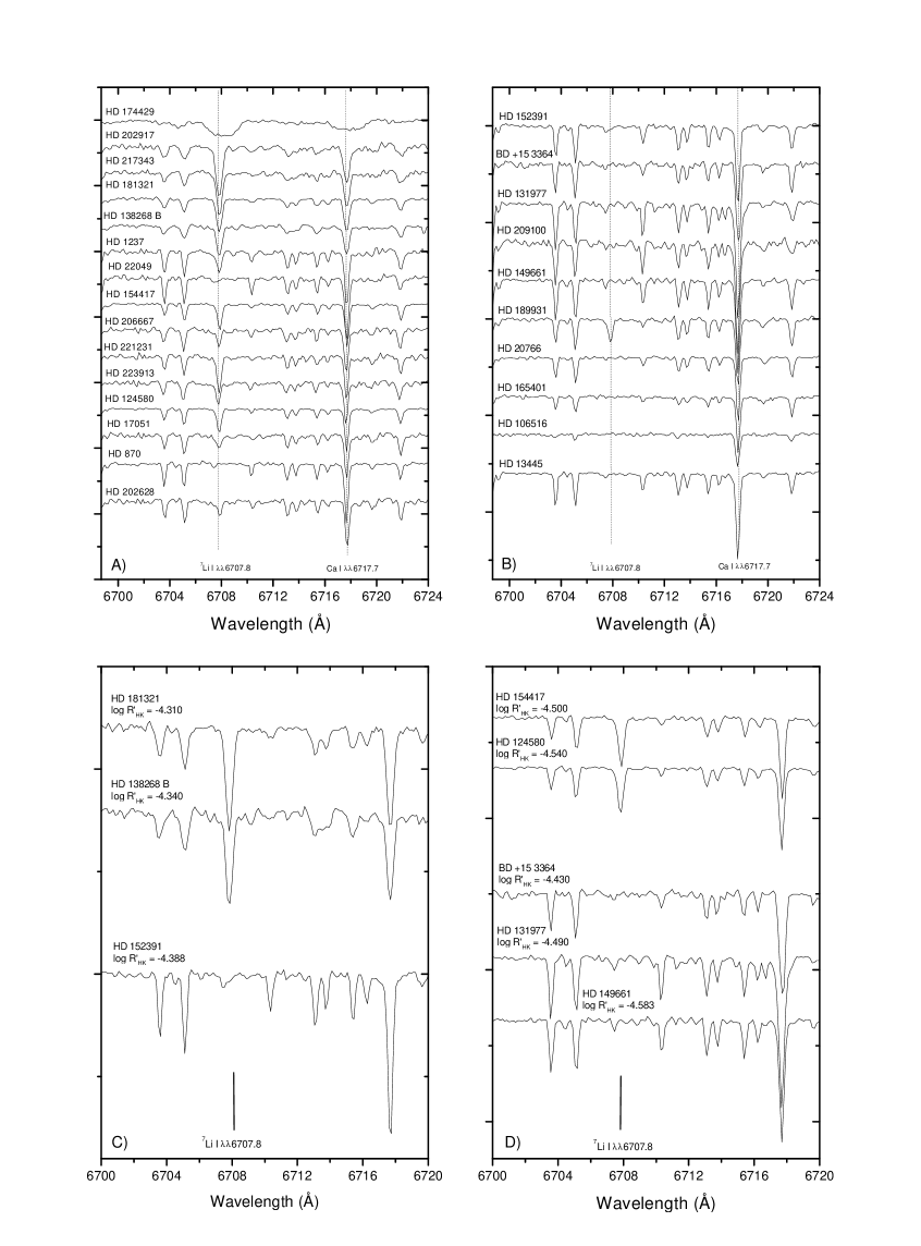
Figure 2: Spectra for active stars in the Li region ($\lambda$ 6707 Å). Panel a presents normal young stars, while panel b presents CYKOS. The spectra are ordered according to the chromospheric activity, with the most active stars in the upper part of the figure. With few exceptions it is seen that the Li line is present in all normal active stars, and its equivalent width becomes smaller towards less active stars. This behaviour is totally absent from the spectra of CYKOS. In panels c and d we compare spectra of stars having the same activity levels and, supposedly, the same age. The upper spectra are for normal stars, in which there is Li. In the bottom spectra, of CYKOS, the Li line is absent.

In Fig. 2a, we show spectra in the Li region ($\lambda$ 6707 Å) for some objects taken as normal. The spectra in this plot are ordered according to the chromospheric activity, the lowest spectra being that of the least active star.

The chromospheric activity order must represent approximately an age order: the most active objects are supposed to be younger than the least active ones. In fact, by inspecting the plot we can see a gradual increase in the equivalent width of the Li line, in going up the Figure, from HD 202628 to HD 174429. The spectrum of HD 185124 was too broadened to allow some comparison with other stars, and was not included in the figure. The presence of lithium and a high chromospheric activity are classical youth indicators in late-type stars. The exceptions are few, and do not contradict this idea. HD 22049 ($\equiv\epsilon$ Eri) is a BY Dra variable, and possibly older than its chromospheric activity suggests. HD 870 has an activity level near that of the Vaughan-Preston gap, and could be considered as an inactive star, observed during a maximum of activity.

The spectra of CYKOS are presented in Fig. 2b. When we examine the same chromospheric activity sequence amongst the CYKOS, we find nothing similar to that found in normal stars. The Li line is only present in the spectra of HD 189931. In the others there is no trace of Li. The comparison can be done more properly in the bottom panels of this figure, where we show normal stars and CYKOS with the same chromospheric activity levels, and supposedly, the same age.

4.3 Stellar Parameters and Models

Stellar parameters (T_eff, $\log g$, [Fe/H]) for the program stars were first derived from the ubvy photometry and the classical relation $\log g_{*}=4.44+4\log T_{*}/T_{\odot}+0.4(M_{\rm bol}-4.74)+\log M_{*}/M_{\odot}$, using the same procedure described in Castilho et al. (cast00 (2000)).

The metallicities of the program stars were then redetermined using curves of growth of Fe I lines where the updated code RENOIR by M. Spite was employed. The stellar parameters used, with the spectroscopic metallicity that we have found, are listed in Table 2. For HD 185124 and HD 174429 a metallicity determination was not possible, due to the line broadening. The error in [Fe/H] is 0.10 dex.

Model atmospheres employed have been interpolated in tables computed with the MARCS code by Edvardsson et al. (edv93 (1993)).

4.4 Li abundances

The Li depletion must not be identical in all observed stars, since it depends on factors such as mass and metallicity. Even the equivalent width of the ⁷Li resonance doublet ($\lambda$ 6707.8Å) depends strongly on the temperature of the star (Castilho et al. cast00 (2000)). Therefore, a strong Li line does not always warrant a high lithium abundance. The stars in Fig. 2 do not have the same temperature, and those plots shall be taken as illustrative comparisons. More accurate estimates of the Li age must be done by considering Li abundances rather than the equivalent widths.

Spectrum synthesis calculations were used to fit the observed spectra of the stars listed in Tab. 2. The calculations of synthetic spectra were carried out using a revised version of the code described in Barbuy (1982), where molecular lines of C₂ (A${}^{3}\Pi$-X${}^{3}\Pi$), CN red (A${}^{2}\Pi$-X${}^{2}\Sigma$) and TiO $\gamma$ (A${}^{3}\Phi$-X${}^{3}\Delta$) systems are taken into account. The oscillator strengths adopted are the laboratory values obtained by Fuhr et al. (fuhr (1988)), Martin et al. (martin (1988)), Wiese et al. (wiese (1969)). When these were not available, we have used those given by Spite et al. (spite (1987)) or Barbuy et al. (barbuy1999 (1999)) obtained by inverse solar analysis. Solar abundances are adopted from Grevesse & Sauval (gs99 (1999)). The derived lithium abundances $N({\rm Li})$ of the observed stars are given in column 10 of Tab. 2.

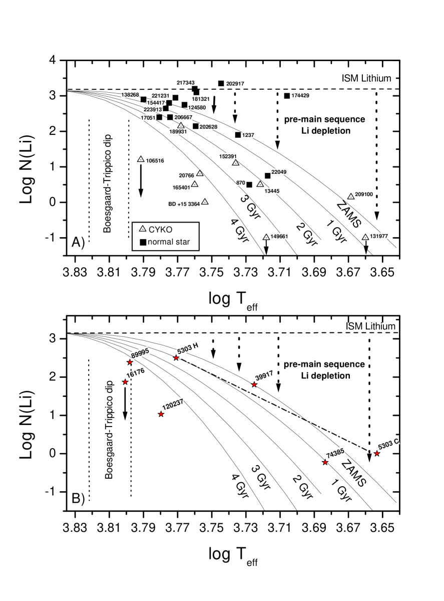
Figure 3: Li depletion diagram for late-type stars, according to Soderblom (soder83 (1983)). Panel a: stars that we have observed; panel b: CYKOS with Li abundances from the literature. In this figure, the dashed horizontal line at the top indicates the Li abundance in the interstellar medium. Vertical arrows correspond to the Li depletion before the main sequence. Several curves indicate the Li depletion expected for stars of a given age. The vertical dotted lines in the left part of the plots correspond to the region of the Boesgaard–Trippico dip.

For the determination of the lithium ages of these stars, we have considered the lithium depletion diagram of Soderblom (soder83 (1983)). Fig. 3 presents a Li depletion diagram as a function of the stellar effective temperature, according to Soderblom (soder83 (1983)). The diagram is an approximation for the calculation of Li ages. The dashed horizontal line corresponds to the Li abundance in the interstellar medium, and the curves indicate the expected depletion as a function of the stellar age. Vertical arrows show the expected lithium depletion before the ZAMS. The vertical dotted lines mark the region corresponding to the Boesgaard–Trippico dip (cf., Boesgaard & Trippico boes (1986)), where depletion is not linked with age, but probably with the internal structure of the star. The filled squares in the top panel of Fig. 3 are the normal young stars of Table 2, while the triangles show the CYKOS. The lower panel of Fig. 3 shows the Li depletion diagram of a few CYKOS (stars) whose abundances are from the literature (section 5). It is clear that normal young stars have lithium abundances very similar to that of the interstellar medium. That is, in these stars there was no depletion. The CYKOS, on the other hand, have Li ages greater than 2 Gyr.

HD 870 is the only exception amongst normal young stars. As mentioned before, this could be an inactive star, included in the sample by an error in $\log R^{\prime}_{\rm HK}$ (for instance, it has been observed in the H an K Ca II lines only once, by Henry et al. HSDB (1996)). HD 189931, in spite of having N(Li) $\ga 2.0$, has the same Li age as HD 152391 and HD 13445.

We conclude that CYKOS present Li ages higher than the ages estimated by their chromospheric activity, although in better agreement with their kinematic properties.

5 Data on individual objects

The initial suggestion by Soderblom (soder90 (1990)) that the CYKOS can be runaway stars seems very unrealistic. If these stars were young, they should present Li abundances typical of their youth. Their high kinematic age is a clear indication of their older status. An initial hypothesis that can be tested is that they could be chromospherically active binaries, which can be tested by searching for radial velocity variations. Before giving a general explanation, it is important to see what is known about the stars in Tab. 1.

HD 5303 $\equiv$ CF Tuc

This is a G0 V + K4 IV RS CVn-type spectroscopic binary (Strassmeier et al. strass (1993)), with an orbital period of 2.80 days. Li abundances were measured by Randich et al. (randich94 (1994)) for both components. In Fig. 3b, both components are linked by a dot-dashed line. Note that this line presents roughly the same slope of the curves with the same Li age.

HD 13445 $\equiv$ HR 637

The index $\log R^{\prime}_{\rm HK}=-4.74$ indicates that this star could be an inactive star. A comparison between H$\alpha$ fluxes (Pasquini & Pallavicini pasquini (1991)) with other stars is ambiguous: HR 13445 presents fluxes similar to HD 42807 and HD 81997 (active stars) and to HD 4308 and the Sun (inactive stars). Favata et al. (favata (1997)) have measured N(Li) $<-0.24$, one order of magnitude lower than our measured value. Queloz et al. (queloz (2000)) have found a planet with 4 Jupiter masses at a distance of 0.11 AU from the star.

HD 16176 $\equiv$ HR 756

This is classified as F5. Balachandran (bal (1990)) measured N(Li) $<1.87$. The depletion would be high for this spectral type, if due to age alone. However, the star is found within the Boesgaard–Trippico dip, and this low lithium abundance cannot be considered as indicative of old age.

HD 20766 $\equiv\zeta_{1}\,\,{\rm Ret}\equiv$ HR 756

This is a G2.5 V star, visual companion of HD 20807, with an angular separation of 307^′′. Wooley (wooley (1970)) suggests that they are members of the $\zeta$ Her moving group, which has an isochrone age of a few billion years. da Silva & Foy (licio (1987)) measured a metallicity typical of population I stars and, therefore, criticized the hypothesis by Johnson et al. (johnson (1968)) that the pair is composed of subdwarfs. There is no sign of radial velocity variability in either stars (da Silva & Foy licio (1987)).

HD 39917 $\equiv$ SZ Pic

This is a RS CVn chromospherically active star (Strassmeier et al. strass (1993)), having an orbital period of 4.80 days. However, Mason et al. (mason (1998)) have not detected a companion within $\Delta V\leq 3.0$ and angular separation between $0.035^{\prime\prime}$ and $1.08^{\prime\prime}$. The lithium abundance was measured by Randich et al. (randich93 (1993)), and is consistent with the expected abundance at the ZAMS (see Fig. 3).

HD 65721

G6 V variable star, ROSAT source (Hünsch et al. huensch98 (1998)). Mason et al. (mason (1998)) have not detected a companion within $\Delta V\leq 3.0$ and angular separation between $0.035^{\prime\prime}$ and $1.08^{\prime\prime}$.

HD 74385

Dwarf K1 V. Favata et al. (favata (1997)) have measured N(Li) $<-0.23$.

HD 88742 $\equiv$ HR 4013

G1 V star, ROSAT source (Hünsch et al. huensch99 (1999)). Mason et al. (mason (1998)) have not detected a companion within $\Delta V\leq 3.0$ and angular separation between $0.035^{\prime\prime}$ and $1.08^{\prime\prime}$.

HD 89995 $\equiv$ HR 4079

F6 V star, ROSAT source (Hünsch et al. huensch99 (1999)). The lithium abundance measured by Balachandran (bal (1990); N(Li) $=2.38$) is high compared to some stars, but small for the temperature of this star (6280 K). The star is located within the Boesgaard–Trippico dip, where depletion is uncorrelated with age.

HD 103431

It is a dG7 star, visual companion of HD 103432, angular separation of 73.2^′′. Constant radial velocity during a time span of 2499 days (Duquennoy & Mayor duc91 (1991)).

HD 106516 $\equiv$ HR 4657

F5 V spectroscopic binary with period of 853.2 days (Latham et al. latham (1992)). Lithium abundance was measured by Lambert et al. (lambert (1991)), N(Li) $<1.32$. The star is also located within the Boesgaard–Trippico dip. Edvardsson et al. (edv93 (1993)) calculate an isochrone age of 5.37 Gyr. Fuhrmann & Bernkopf (fuhrmann (1999)) suggest that this star is a field blue straggler, having a chemical composition and kinematics typical of thick disk stars, in spite of having an age typical of thin disk stars.

HD 120237 $\equiv$ HR 5189

It is classified as G3 IV-V. There is no indication of a companion within $\Delta V\leq 3.0$ and angular separation between $0.035^{\prime\prime}$ and $1.08^{\prime\prime}$ (Mason et al. mason (1998)). The lithium abundance was calculated by Randich et al. (randich99 (1999)), N(Li) $=1.03$. The depletion seems substantial for the temperature of this star.

HD 123651

There is no indication of a companion within $\Delta V\leq 3.0$ and angular separation between $0.035^{\prime\prime}$ and $1.08^{\prime\prime}$ (Mason et al. mason (1998)).

HD 131977

K4 V visual binary, with angular separation of 20^′′. The companion is HD 131976. Its x-ray emission level is moderate (Wood et al. wood (1994)), but there seems to be no doubt about its activity (Robinson, Cram & Giampapa robin (1990)). Duquennoy & Mayor (duc88 (1988)) have found no invisible companion for this star.

HD 149661 $\equiv$ 12 Oph $\equiv$ V2133 Oph $\equiv$ HR 6171

K2 V variable of BY Dra type (Petit petit (1990)). It was detected by ROSAT in EUVE with moderate intensity (Tsikoudi & Kellett tsil (1997)). Habing et al. (habing (1996)) report a Vega-like protoplanetary disk, but the presence of cirrus during the observation has somewhat made this finding inconclusive. Young, Mielbrecht & Abt (young (1987)) and Tokovinin (tokovin (1992)) have found a constant radial velocity for this star, and McAlister et al. (mcallister (1987)) did not detect the presence of an unseen companion by using speckle interferometry.

HD 152391 $\equiv$ V2292 Oph

G8 V variable star of BY Dra type (Petit petit (1990)). Detected by ROSAT in EUVE with moderate intensity (Tsikoudi & Kellett tsil (1997)). Constant radial velocity during a timespan of 3387 days (Duquennoy & Mayor duc91 (1991)).

HD 165401

It is a G0 V, relativaly metal-poor star ([Fe/H] $\sim-0.50$ dex). The index $\log R^{\prime}_{\rm HK}$ that we have used refers to a sole observation (Duncan et al. duncan (1991)). We have considered the possibility that this star is inactive, but its emission in H$\alpha$ (Herbig herbig (1985)) seems consistent with its $\log R^{\prime}_{\rm HK}$. There is no unseen companion with a magnitude diference lower than 2.5 mag and angular separation greater than 3 AU, according to speckle interferometry (Lu et al. lu-patinadora (1987)). Abt & Levy (abtlevy (1969)) have found a radial velocity variability of $\pm 5$ km/s, but recent investigations do not confirm this result (Duquennoy & Mayor duc91 (1991); Abt & Willmarth abtwill (1987)). Curiously, radial velocities measured for this star during the sixties and seventies yield values homogeneously around $v_{r}\approx-114$ km/s, while all recent studies yield values around $v_{r}\approx-120$ km/s.

HD 196850

G2 V star, with constant radial velocity during a time span of 3995 days (Duquennoy & Mayor duc91 (1991)).

BD +15 3364

Solar-metallicity G0 V star. Duquennoy & Mayor (duc91 (1991)) have found a constant radial velocity during a time span of 2264 days. Carney (carney (1983)) found no photometric variability characteristic of an unseen companion.

6 The nature of CYKOS

6.1 Coalescence of close binaries

The majority of objects considered in the previous section are undoubtedly active, have lithium abundances lower than that of stars with 2 Gyr of age, and some show no indication of radial velocity variations. They are thus single objects, most probably old.

As we have seen, some of them are chromospherically active binaries. Their chromospheric activity results from the synchronization of the orbital with the rotational motion. This is the reason why they have a low chromospheric age, but a higher age from the point of view of their kinematics. Nevertheless, in the case of single stars, there is no known mechanism that could store angular momentum to be used later by the star. The anomalously low lithium abundance, together with the high velocity components, are hardly interpreted as a consequence of anything but an old age. Even the BY Dra variables in the sample must be single stars, and not chromospherically active binaries, since there is no indication of variability in $v_{r}$ for them. Amongst BY Dra stars are found binaries as well as single stars (Eker eker (1992)). Soderblom (soder90 (1990)) has estimated a kinematic age of 1-2 Gyr for them, contrary to the expectation that these stars could keep high activity levels at advanced ages. The low kinematic age must be understood as an evidence that the BY Dra-type variability is not exclusive of chromospherically active stars, but could be generated by the intensity of the magnetic activity itself amongst low-mass stars, binaries or not.

Poveda et al. (1996a ,b) also have found several CYKOS amongst UV Ceti stars, which are known as young low-mass stars. The authors suggest that these objects could be red stragglers, a low-mass analogous of the well-known blue stragglers. According to this hypothesis, the red stragglers would be produced by the coalescence of two low-mass stars (with about 0.5 $M_{\odot}$ each) originally in a short-period binary pair. According to them, these objects would be stragglers in a velocity diagram, compared to other stars. However, being more rapid, they would not be stragglers in the sense they are in the HR diagram. Thus, the name ‘field blue stragglers’ includes not only the idea about their origin, but also their present location out of a cluster. Note that the same denomination was used by Fuhrmann & Bernkopf (fuhrmann (1999)).

The coalescence scenario was already considered as a classic explanation for the formation of blue stragglers. Two works (van’t Veer & Maceroni vant (1989); Stȩpień stepien (1995)) that investigate the coalescence of short-period binaries into a single star predict the formation of low-mass blue stragglers. Stȩpień (stepien (1995)) has even shown that the coalescence is more easily attained for low-mass binaries (each having around 0.6 $M_{\odot}$, forming a star with 1.2 $M_{\odot}$) than for more massive stars that originate the classic blue stragglers in open clusters. The formation of a low-mass blue straggler could be achieved within 2.5 Gyr, for systems having an initial orbital period of 2 days.

The properties of a supposed low-mass field blue straggler would be tightly similar to that of some CYKOS, as we will see in what follows.

In short-period binaries, we expect the occurrence of synchronization between the orbital and rotational periods. For low-mass stars, the magnetic activity is strong, and increases the angular momentum loss. When both orbital and rotational periods are synchronized, the rotational angular momentum loss occurs at the expenses of the orbital angular momentum. As a result, the period decreases, the components rotate more rapidly, and become closer to each other, eventually becoming contact binaries, as those of W UMa-type.

Rasio & Shapiro (rasio (1995)) simulate systems like these, using the technique of smooth particle hydrodynamics. The authors show that once the contact is achieved, these systems are dynamically unstable and can rapidly coalesce into a single object, having a high rotation rate. The events related to this coalescence can produce an extense outer envelope that would make the star appear like a pre-main sequence star. According to the authors, the coalescence can occur in a time scale of a few hours, once the dynamical instability is set. The envelope is kept gravitationally bound to the star, which eventually contracts towards thermal equilibrium. Mass loss, in this event, would be minimal.

In a coalescence of two low-mass stars (0.5 $M_{\odot}$ each), the resulting star must present a mass similar to that of the Sun and a high rotation rate. This rotation rate, together with the convection in the outer stellar atmosphere, would produce a copious chromospheric activity, similar to the one found in very young stars. In the case of low-mass stars that have not ignited hydrogen in their cores, the just formed single star would be similar in many respects to a young star, positioning in the zero-age main sequence, like the blue stragglers. However, this star would inherit the same velocity components of the binary pair from which it was formed. Thus, due to the time before the coalescence, the velocity components are not similar to that of a young star. We would have a star almost in everything young, but kinematically old. The lithium abundance is also one of the few tracks that can show the real nature of these objects. In spite of not burning hydrogen considerably, stars having around 0.5 $M_{\odot}$ are highly convective, and Li burning is very efficient in them. Blue Stragglers like these should present small or no Li abundance (Pritchet & Glaspey pritchet (1991); Glaspey et al. glaspey (1994)), since they would be formed by older objects.

A criticism that could be made is that, if CYKOS are field blue stragglers, formed during the coalescence of low-mass short-period binaries, why do their spectra not present very broad lines, as it is expected in stars with high rotation rates? The same problem occurs for blue stragglers in open and globular clusters, that do not rotate more rapidly than young normal stars. Leonard & Livio (leonard (1995)) suggest that the majority of the angular momentum is stored in the extense disk that is formed around just formed blue stragglers. The central object would expand, due to the thermal energy resulting from the coalescence, and contracts toward thermal equilibrium, in a time scale lower than 10⁷ years, similar to that of pre-main sequence stars. Thus, we do not find CYKOS with broader lines simply because we do not expect that they all have been formed within the last 0.5 Gyr.

Seven amongst our stars seem to fit well within these criteria: HD 20766, HD 106516, HD 131977, HD 149661, HD 152391, HD 165401, BD +15 3364. Other stars are suspect, but the information is insufficient to characterize them as low-mass blue stragglers. One of the stars (HD 189931) seems to be a real young single object with high velocity components (see also Tab. 1). Nevertheless, there is little information in the literature that could test this hypothesis. The other stars need more data to investigate whether they are field blue stragglers, chromospherically active stars or runaway stars.

6.2 Coalescence Rate

The formation rate of these objects can be calculated from considerations about the initial mass function, star formation rate, initial period distribution in binaries and the time scale for contact. The time needed for the coalescence, once contact is achieved, is very small compared to the time scale for contact (Rasio & Shapiro rasio (1995)), and we will consider it negligible.

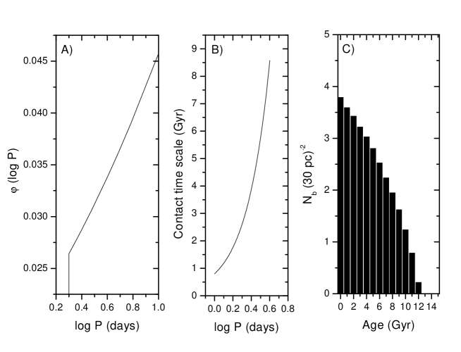
Figure 4: Calculations for the formation rate of population I field blue stragglers having masses between 0.8-1.2 $M_{\odot}$. Panel a: initial period distribution, adapted from Duquennoy & Mayor (duc91 (1991)); panel b: time scale for contact; panel c: number of field blue stragglers, with mass in the considered range, formed within a sphere of 30 pc radius centred at the Sun.

It can be shown that the total number of stars, having masses between $m_{1}$ and $m_{2}$, that becomes contact binaries in $t$ is

$$N_{b}(t)=b\int^{{m_{2}}}_{{m_{1}}}\int^{\infty}_{0.3}\int^{0.5}_{0}{{\cal P}}(\mu,\log P,m,t)\,{\rm d}\mu\,{\rm d}\log P\,{\rm d}m$$ (1)

$${{\cal P}}(\mu,\log P,m,t)=f(\mu)\varphi(\log P)\psi(t-\tau_{\mu Pm})\phi(m),$$ (2)

where $\tau_{\mu Pm}$ is the time scale for contact for a binary, having initial period in the range $(\log P,\log$ $P+\Delta\log P)$, secondary-to-total mass ratio between $(\mu,\mu+\Delta\mu)$ and total mass between $(m,m+\Delta m)$, $\varphi(\log P)$ is the initial period distribution, $f(\mu)$ is the distribution of mass ratio, $\psi(t)$ is the star formation rate, and $\phi(m)$ is the initial mass function.

For the computation of the equation above, we will consider $\varphi(\log P)\approx 0.018+0.027\log P$, with a cutoff for $\log P<0.3$, which approximates fairly well the initial period distribution of Duquennoy & Mayor (duc91 (1991)), for the region $0.3<\log P<1.0$, where $P$ is in days. We have assumed $f(\mu)=24\mu^{2}$ (Matteucci & Greggio greggio (1986)), $m_{1}=0.8M_{\odot}$ and $m_{2}=1.2M_{\odot}$, which correspond to pairs having total masses equal to the mass range for G dwarfs.

The function $\tau_{\mu Pm}$ is very complicated. Stȩpień (stepien (1995)) published calculations for only three binary configurations: $1M_{\odot}+1M_{\odot}$, $1M_{\odot}+0.65M_{\odot}$ and $0.6M_{\odot}+0.6M_{\odot}$. The last of these has total mass equal to $m_{2}$, but calculations for lower total masses are not published, neither for different $\mu$. However, Stȩpień says that configurations for lower total masses achieve contact in a time scale lower than that for the system $0.6M_{\odot}+0.6M_{\odot}$. We consider that $\tau_{\mu Pm}$ can be approximated by a function $\tau_{P}$, which depends only on the initial period, and that is given by the time for contact for the system $0.6M_{\odot}+0.6M_{\odot}$. Note that being $\tau_{P}$ a maximum time scale, our estimates will be a little underestimated, since the total number of systems that have achieved contact $\tau_{P}$ after the formation of the binary will be greater that the calculated number, due to the number of binaries with lower total masses that achieve contact more rapidly. Also, due to the initial mass function, the number of systems with lower total masses must be higher. Taken these into account, Eq. 1 reduces to $N_{b}(t)\ga cF(t)$, where

$$c=b\int^{1.2}_{0.8}\phi(m)\,{\rm d}m$$ (3)

and

$$F(t)=\int^{\infty}_{0.3}\varphi(\log P)\psi(t-\tau_{P})\,{\rm d}\log P,$$ (4)

since the integral in $\mu$ is unity.

For the calculation of $\tau_{P}$, we have considered Fig. 2 of Stȩpień (stepien (1995)). The time scales for contact were fitted by $\tau_{P}=0.8e^{4\log P}$. We have assumed a constant star formation rate, in spite of the evidences for its non-constancy (Rocha-Pinto et al. 2000b ), since we are only interested in the magnitude of the coalescence rate.

In Fig. 4a, the initial period distribution is shown. The time scale for contact is shown in panel b. The number of field blue stragglers already formed was calculated for a sphere of radius 30 pc around the Sun, which correspond approximately to the volume within which our sample is nearly complete. This rate is shown in Fig. 4c. Integrating the data in this panel, we have a total number of 28 blue stragglers already formed in this sphere.

The calculations are very rough, as can be seen from the approximations considered. However, the number of objects formed in the sphere is similar in order of magnitude to the number of field blue stragglers in our sample (including suspect objects). This reinforces our hypothesis for the nature of these objects.

From these results, we believe to have found population I field blue stragglers. Poveda et al. (1996a ,b) arise a hypothesis that cannot be tested with the same probability level as ours, since they do not have an indication of old age for their stars, besides their kinematics.

The traditional method used for finding a blue straggler, based on its position in the HR diagram, is not possible to be used for a population I field blue straggler. The search for objects with strong chromospheric activity, or little Li, or with high velocity, also do not allow their identification, since normal stars present these properties. Only by the intersection of several properties we have found objects which apparently can be best explained by this scenario.

It is worth mentioning an independent research on ultra-lithium-deficient halo stars recently published by Ryan et al. (ryan (2001)), which conclude that such stars can have the same origin of the blue stragglers, being their lower mass the only significant difference between them.

- (1) Abt H.A., Levy S.G., 1969, AJ 74, 908
- (2) Abt H.A., Willmarth D.W., 1987, ApJ 318, 786
- (3) Balachandran S., 1990, ApJ 354, 310
- (4) Barbuy B., 1982, Ph.D. Thesis, Univ. Paris VII
- (5) Barbuy B., Renzini A., Ortolani S., Bica E. 1999, A&A 341, 539
- (6) Bertelli G., Bressan A., Chiosi C., Fagotto F., Nasi, E., 1994, A&AS 106, 275
- (7) Boesgaard A.M., Tripicco M.J., 1986, ApJ 302, L49
- (8) Carney B.W., 1983, AJ 88, 623
- (9) Castilho B.V., Gregorio-Hetem J., Spite F., Barbuy B., Spite M. 2000, A&A 364, 674
- (10) Cayrel de Strobel G., 1974, in Highlights of Astronomy, 3 , 369
- (11) da Silva L., Foy R., 1987, A&A 177, 204
- (12) Duncan D.K., Vaughan A.H., Wilson O. C., et al., 1991, ApJS 76, 383
- (13) Duquennoy A., Mayor M., 1988, A&A 200, 135
- (14) Duquennoy A., Mayor M., 1991, A&A 248, 485
- (15) Edvardsson B., Andersen J., Gustafsson B. et al., 1993, A&A 275, 101
- (16) Eker Z., 1992, ApJS, 79, 481
- (17) Favata F., Micela G., Sciortino S., 1997, A&A 322, 131
- (18) Fuhr J.R., Martin G.A., Wiese W.L., 1988, Journal of Physical and Chemical Reference Data, vol. 17, suppl. 4
- (19) Fuhrmann K., Bernkopf J., 1999, A&A 347, 897
- (20) Glaspey J.W., Pritchet C.J., Stetson P.B., 1994, AJ 108, 271
- (21) Grevesse N., Sauval A.J., 1999, A&A 347, 348
- (22) Habing H.J., Bouchet P., Dominik C., et al., 1996, A&A 315, L233
- (23) Henry T.J., Soderblom D.R., Donahue R.A., Baliunas S.L., 1996, AJ 111, 439
- (24) Herbig G.H., 1985, ApJ 294, 310
- (25) Hünsch M., Schmitt J.H.M.M., Sterzik M.F., Voges W., 1999, A&AS 135, 319
- (26) Hünsch M., Schmitt J.H.M.M., Voges W., 1998, A&AS 127, 251
- (27) Jeffries R.D., Jewell S.J., 1993, MNRAS, 264, 106
- (28) Johnson H. L., MacArthur J. W., Mitchell R. I., 1968, ApJ 152, 465
- (29) Johnson D.R.H., Soderblom D.R., 1987, AJ 93, 864
- (30) Lambert D.L., Heath J.E., Edvardsson B., 1991, MNRAS 253, 610
- (31) Latham D.W., Mazeh T., Stefanik R.P., Davis R.J., Carney B.W., Krymolowski Y., Laird J.B., Torres G., Morse J.A., 1992, AJ 104, 774
- (32) Leonard P.J.T., Livio M., 1995, ApJ 447, L121
- (33) Lu P.K., Demarque P., Van Altena W., McAlister H., Hartkopf W., 1987, AJ 94, 1318
- (34) Martin G.A., Fuhr J.R., Wiese W.L., 1988, Journal of Physical and Chemical Reference Data vol. 17, suppl. no. 3
- (35) Mason B.D., Henry T.J., Hartkopf W.I., ten Brummelaar T., Soderblom D.R., 1998, AJ 116, 2975
- (36) Matteucci F., Greggio L., 1986, A&A 154, 279
- (37) McAllister H.A., Hartkopf W.I., Hutter D.J., Shara M.M., Franz O.G., 1987, AJ 93, 183
- (38) Meusinger H., Reimann H.-G., Stecklum B., 1991, A&A, 245, 57
- (39) Mihalas D., Binney J., 1981, Galactic Astronomy, W.H. Freeman and Co., San Francisco
- (40) Noyes R.W., Hartmann L.W., Baliunas S.L., Duncan D.K., Vaughan A.H., 1984, ApJ 279, 778
- (41) Olsen E.H., 1984, A&AS 57, 443
- (42) Palouš J., Bull. Astron. Inst. Czech., 1983, 34, 286
- (43) Pasquini L., Pallavicini R., 1991, A&A 251, 199
- (44) Petit M., 1990, A&AS 85, 971
- (45) Poveda A., Allen C., Herrera M.A., Cordero G., Lavalley C., 1996a, A&A 308, 55
- (46) Poveda A., Allen C.., Herrera M.A., 1996b, RMA&A Conf. Ser., 5, 16
- (47) Pritchet C.J., Glaspey J.W., 1991, ApJ 373, 105
- (48) Randich S., Giampapa M.S., Pallavicini R., 1994, A&A 283, 893
- (49) Randich S., Gratton R., Pallavicini R., 1993, A&A 273, 194
- (50) Randich S., Gratton R., Pallavicini R., Pasquini L., Caretta E., 1999, A&A 348, 487
- (51) Rasio F.A., Shapiro S.L., 1995, ApJ 438, 887
- (52) Queloz D., Mayor M., Weber L., Blécha A., Burnet M., Confino B., Naef D., Pepe F., Santos N., Udry S., 2000, A&A 354, 99
- (53) Robinson R.D., Cram L.E., Giampapa M.S., 1990, ApJS 74, 891
- (54) Rocha-Pinto H.J., Maciel W.J., 1998, MNRAS, 298, 332
- (55) Rocha-Pinto H.J., Maciel W.J., Scalo J., Flynn C., 2000a, A&A, 358, 850
- (56) Rocha-Pinto H.J., Scalo J., Maciel W.J., Flynn C., 2000b, A&A, 358, 869
- (57) Rocha-Pinto H.J., Flynn C., Scalo J., Maciel W.J., 2002, in preparation
- (58) Ryan S.G., Beers T.C., Kajino T., Rosolankova K., 2001, ApJ, 547, 231
- (59) Soderblom D.R., 1983, ApJS 53, 1
- (60) Soderblom D.R., 1990, AJ 100, 204
- (61) Soderblom D.R., King J.R., Henry T.J., 1998, AJ 116, 396
- (62) Spite M., Huille S., François P., Spite F. 1987, A&AS 71, 591
- (63) Stȩpień K., 1995, MNRAS 274, 1019
- (64) Strassmeier K.G., Hall D.S., Fekel F.C., Scheck M., 1993, A&AS 100, 173
- (65) Tokovinin A.A., 1992, A&A 256, 121
- (66) Tsikoudi V., Kellett B.J., 1997, MNRAS 285, 759
- (67) van’t Veer F., Maceroni C., 1989, A&A 220, 128
- (68) Wielen R., 1974, in Highlights of Astronomy, 3 , 395
- (69) Wiese W.L., Martin G.A., Fuhr J.R., 1969, Atomic Transition Probabilities: Sodium through Calcium. NSRDS-NBS 22
- (70) Wood B.E., Brown A., Linsky J.L., Kellett B.J., Bromage G.E., Hodgkin S.T., Pye J.P., 1994, ApJS 93, 287
- (71) Wooley R.v.d.R., 1970, in Galactic Astronomy, H.Y.Chiu, A.Muriel, eds., Gordon & Breach, New York, 95
- (72) Young A., Mielbrecht R.A., Abt H.A., 1987, ApJ 317, 787