Empirical calibration of the near-infrared Ca II triplet – III. Fitting functions

Abstract

Using a near-IR stellar library of 706 stars with a wide coverage of atmospheric parameters, we study the behaviour of the Ca ii triplet strength in terms of effective temperature, surface gravity and metallicity. Empirical fitting functions for recently defined line-strength indices, namely CaT^∗, CaT and PaT, are provided. These functions can be easily implemented into stellar populations models to provide accurate predictions for integrated Ca ii strengths. We also present a thorough study of the various error sources and their relation to the residuals of the derived fitting functions. Finally, the derived functional forms and the behaviour of the predicted Ca ii are compared with those of previous works in the field.

1 Introduction

This is the third paper in a series dedicated to the understanding of stellar populations of early–type galaxies and other stellar systems by using their near–IR spectra and, particularly, the strength of the integrated Ca ii triplet. In the previous papers, we have presented the basic ingredients of this project. First, we have observed a new stellar library of 706 stars at 1.5 Å (FWHM) spectral resolution in the range $\lambda\lambda$ 8348-9020 Å (Cenarro et al. 2001a, Paper I). That paper also includes the definition of 3 new, improved line-strength indices in the Ca ii triplet region (namely CaT, PaT, CaT^∗), which are especially suited to be measured in the integrated spectra of stellar populations. Paper II of the series (Cenarro et al. 2001b) presents an updated set of atmospheric parameters ($T_{{\rm eff}}$, $\log g$ and [Fe/H]) for the stars of the library. The objective of this third paper is to provide empirical fitting functions describing the behaviour of the above indices in terms of the atmospheric parameters. Together with the spectra of the stellar library, the fitting functions will be implemented into an evolutionary stellar populations synthesis code to predict both the spectral energy distribution and the strengths of the indices for stellar populations of several ages and metallicities (Vazdekis et al. 2001, Paper IV).

A popular method to investigate the star formation history and the stellar content of galaxies is to compare observed line strength indices with stellar population models. This requires an accurate, prior knowledge of the behaviour of the spectral features of interest for a wide range of stellar spectral types, luminosity classes and metallicities, which can be accomplished with the aid of either empirical stellar libraries or theoretical model atmospheres. There are two common alternatives for the stellar populations synthesis approach. The first method mixes the spectra of the different stars with their relative ratios given by evolutionary synthesis models to predict spectral energy distributions (Fioc & Rocca-Volmerange 1997; Leitherer et al. 1999; Vazdekis 1999; Schiavon, Barbuy & Bruzual 2000; Bruzual & Charlot 2001). The major advantage of this spectral synthesis is that it provides full information of all the spectral features within the spectral range covered by the stellar library. However, its usefulness relies on the availability of a complete stellar library at the appropriate spectral resolution. The second procedure, and probably the most widely employed in the past, is the use of empirical fitting functions describing the strength of previously defined spectral features in terms of the main atmospheric parameters. These calibrations are directly implemented into the stellar populations models to derive the index values for populations of different ages and metallicities. It must be noted that one of the main advantages of using fitting functions to reproduce the behaviour of spectral indices is that it allows stellar populations models to include the contribution of all the required stars by means of smooth interpolations between well-populated regions in the parameter space. One should not forget that, in any of the above two methods, a common limitation of the empirical procedures arises from the fact that they implicitly include the chemical enrichment history of the solar neighborhood. This caveat must be kept in mind when using model predictions to interpret the stellar populations of external galaxies, whose star formation histories might be completely different to that of the Galaxy.

The usefulness of the fitting functions approach has been clearly demonstrated by the fact that the most important evolutionary synthesis models (e.g., Worthey 1994, Vazdekis et al. 1996, Tantalo et al. 1996 or Bruzual & Charlot 2001) have implemented the available fitting functions to fit observed line strengths in the literature. Unfortunately, at present fitting functions are only available in the blue and visible part of the spectrum (e.g. Gorgas et al. 1993, Worthey et al. 1994 and Worthey & Ottaviani 1997 for the Lick/IDS indices; Poggianti & Barbaro 1997 and Gorgas et al. 1999 for the $\lambda$ 4000Å break). Since other spectral regions also contain very useful, complementary, absorption lines, it is necessary to extend this kind of calibrations to line-strength indices in other spectral regimes, such as the ultraviolet and the near infrared (e.g. the CO index at 2.2 $\mu$m analyzed by Doyon, Joseph & Wright 1994). This is indeed an important motivation for this paper. So, before we give a comprehensive analysis of the predictions of both the spectral synthesis and the fitting functions for stellar populations (Paper IV), we will concentrate in this paper on understanding the behaviour of the Ca ii triplet as a function of the atmospheric parameters, providing the corresponding fitting functions.

The Ca ii triplet is one of the most prominent features in the near-IR region of the spectrum of cool stars. Even though there are many previous works dealing with the near-IR Ca ii triplet (we refer the reader to the short review presented in Section 2 of Paper I), the papers by Díaz, Terlevich & Terlevich (1989), Zhou (1991), J$\o$rgensen, Carlsson & Johnson (1992) and Idiart, Thevenin & de Freitas-Pacheco (1997) (hereafter DTT, ZHO, JCJ and ITD, respectively) deserve a special mention, since they provide empirical fitting functions for the Ca ii triplet. They have been very useful to obtain a first understanding of the behaviour of the Ca ii triplet as a function of the stellar parameters but, as we will see in this paper, suffer from several limitations that make it impossible for stellar populations models to predict reliable calcium strengths, especially for old stellar populations. Previous papers which have made use of the above mentioned fitting functions to predict the Ca ii triplet in the integrated spectra of galaxies include Vazdekis et al. (1996), ITD, Mayya (1997), García–Vargas, Mollá & Bressan (1998), Leitherer et al. (1999) and Mollá & García–Vargas (2000).

Section 2 of this paper describes the qualitative behaviour of the Ca ii triplet as a function of the atmospheric parameters, as derived from the new stellar library. We also include a comparison with the results of the previous work. We devote Section 3 to the mathematical fitting procedure, providing the significant terms, coefficients and statistics of the derived fitting functions. Afterwards, a thorough analysis of residuals and possible error sources is presented, including the sensitivity of the fitting functions to differences in Ca/Fe ratios. In Section 4, we compare the new fitting functions with those presented in previous papers. Finally, Sections 5 is reserved to discuss some important issues and to summarize the contents of this paper.

2 Behaviour of the Ca ii triplet as a function of atmospheric parameters

Figure 1: Sequences in spectral types for (a) dwarf and (b) giant stars from the near-IR stellar library. Effective temperatures, names, spectral types, luminosity classes and surface gravities ($\log g$ in dex) are given in the labels. All the spectra have been normalized and reproduced using the same scales so relative differences among the spectra are kept.

Figure 2: Metallicity and gravity effects on the strength of the Ca ii triplet for a subsample of stars from the near-IR stellar library. Panel (a) shows stars with similar temperature and gravity but spanning a wide range in metallicity. Panel (b) displays a sequence in gravity for stars with similar temperature, and metallicity around solar. Temperatures in K are given in brackets. All the spectra have been normalized and reproduced using the same scale.

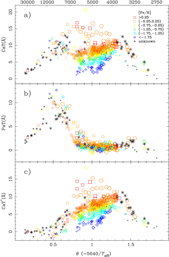
Figure 3: CaT, PaT and CaT${}^{*}(={\rm CaT}-0.93{\rm PaT})$ indices versus $\theta(\equiv 5040/T_{\rm eff})$ for the whole stellar library. Different symbols are used to indicate different metallicities (as in the key), while sizes are related with surface gravity, in the sense that the larger the symbol (supergiants), the lower the gravity. On the top, the effective temperature scale is given.

2.1 Qualitative behaviour

As a first step to understand the behaviour of the Ca ii triplet as a function of the atmospheric parameters, this section describes, from a qualitative point of view, the effect of temperature, surface gravity and metallicity on the strength of the Ca ii lines. Figure 1 shows a comparative sequence in spectral types for a sample of dwarfs (a) and giants (b) taken from the new near-IR stellar library (see also Figure 1 in Paper I for a detailed description of the strongest spectral features). The effects of metallicity and gravity on the Ca ii lines are clearly shown in Figure 2. In Figure 3 we plot the measured CaT, PaT and CaT^∗ indices versus $\theta$ ($\equiv 5040/T_{\rm eff}$) for the whole sample of stars.

Table 1: Bandpass limits for the generic indices CaT and PaT.

CaT central	PaT central	Continuum
bandpasses (Å)	bandpasses (Å)	bandpasses (Å)
Ca1 8484.0–8513.0	Pa1 8461.0–8474.0	8474.0–8484.0
Ca2 8522.0–8562.0	Pa2 8577.0–8619.0	8563.0–8577.0
Ca3 8642.0–8682.0	Pa3 8730.0–8772.0	8619.0–8642.0
		8700.0–8725.0
		8776.0–8792.0

It is worth reminding that the indices CaT and PaT measure, respectively, the strengths of the raw calcium triplet and of three pure H Paschen lines. They consist of five continuum bandpasses (which are the same for both indices) and three central bandpasses covering, in each case, the three Ca ii lines (CaT) or the P17, P14 and P12 lines of the Paschen series (PaT). Table 1 lists the bandpass limits of these indices. The PaT index was specially designed to quantify the CaT contamination with Paschen lines, and it makes it possible to define the corrected index CaT${}^{*}(={\rm CaT}-0.93{\rm PaT})$ as a reliable indicator of the pure Ca ii strength. We refer the reader to Paper I for further details about the definition and measurement of the above indices.

The spectra of hot stars (Fig. 1, top) are dominated by Paschen lines, whose relative depths exhibit a smooth sequence with wavelength, with the Ca ii strengths, both in dwarfs and giants, being clearly negligible (see also Fig. 3c). As temperature decreases, the Ca ii lines become prominent, standing out over the Paschen lines sequence (see the A and F types in Fig. 1). The increasing strength of the Ca ii index with the decreasing temperature peaks at late K and early M types. For a wide range of spectral types ($0.7\leq\theta\leq 1.2$), the Ca ii lines are heavily affected by metallicity and gravity effects (leading to the large spread of CaT and CaT^∗ values in Figs. 3a and  3c), in the sense that their strengths increase as metallicity increases and gravity decreases (Fig. 2). For lower temperatures, Ca goes gradually into a neutral state and the Ca ii strength decreases. The turning point at which the trend with temperature changes depends on the luminosity class, being cooler for giants ($\theta\sim 1.3$) than for dwarfs ($\theta\sim 1.1$). Such an effect is readily seen in Figs. 3a and  3c, and also by comparing the depths of the Ca ii lines for the M4 V and M4 III types in Fig. 1. Finally, strong molecular bands of TiO and VO dominate the latest spectral types, in which the Ca ii strength is almost negligible (Fig. 1, bottom). For these stars, as well as for the very hot ones, metallicity seems not to affect the calcium strength.

The behaviour of the PaT index is illustrated in Fig 3b. As expected for a hydrogen index, it attains high values for hot and warm stars ($\theta\la 0.8$), showing a maximum at an effective temperature which depends on the luminosity class (already reported by Andrillat, Jaschek & Jaschek 1995). Even though, in the low temperature regime, the stellar spectra do not present Paschen lines, the index takes values slightly larger than zero. This is mainly due to the contamination of weak metallic lines falling within the central bands. Also, the presence of strong molecular bands in the spectra of cold giants ($\theta\ga 1.4$) causes a fictitious enlargement of the PaT values.

2.2 Comparison with previous work

In Paper I we have already presented a brief review of the previous work studying the Ca ii triplet as a function of atmospheric parameters. To facilitate the following discussion, in Table 2 we give a summary of the conclusions of these previous studies. We include the main empirical papers on the subject, together with the theoretical calibration of JCJ. Columns 3 to 5 give the ranges of the atmospheric parameters spanned by the calibrating stars (the numbers of stars used are listed in column 2) or atmosphere models. The atmospheric parameters on which the Ca ii triplet was found to be dependent in these previous works are indicated in columns 6 to 8, where the keywords strong and weak are used to remark that the Ca ii strength was reported to be more sensitive to one parameter than to another.

Table 2: Previous calibrations of the Ca ii triplet. Sources are the following: JAJ (Jones, Alloin & Jones 1984), CVP (Carter, Visvanathan & Pickles 1986), A&B (Alloin & Bica 1989), DTT (Díaz, Terlevich & Terlevich 1989), ZHO (Zhou 1991), MAL (Mallik 1997), ITD (Idiart, Thévenin & de Freitas Pacheco 1997), and JCJ (Jørgensen, Carlsson & Johnson 1992).

Source	No.	$\theta$	$\log g$	[Fe/H]	$T_{\rm eff}$	$g$	[Fe/H]	Fitting functions
	stars	range	range	range	dependences			parameters
JAJ	62	$0.68-1.47$	$0.7-4.8$	$-0.60-+0.43$	no	strong	weak
CVP	51	$0.93-1.68$	$0.0-4.6$	$0-+0.50$	yes	yes	no
A&B	63	$0.68-1.46$	$0.7-4.8$	$-0.60-+0.43$	?	yes	yes
DTT	106	$0.74-1.43$	$0.2-4.6$	$-2.70-+0.55$	no	yes	yes	$\log g$, [Fe/H]
ZHO	144	$0.76-1.72$	$0.7-4.8$	$-2.28-+0.60$	yes	yes	yes	$(R-I)$, $(R-I)^{2}$, $\log g$, $\log^{2}g$, $10^{\rm[Fe/H]}$
MAL	146	$0.81-1.58$	$-0.6-4.8$	$-3.0-+1.01$	weak	yes	yes
ITD	67	$0.74-1.20$	$0.8-4.5$	$-3.15-+0.35$	yes	weak	strong	$\theta$, $\log g$, [Fe/H], $\theta{\rm[Fe/H]}$, $\log g{\rm[Fe/H]}$, [Ca/Fe]
JCJ	–	$0.76-1.26$	$0.0-4.0$	$-1.0-+0.20$	yes	yes	yes	$T_{\rm eff}$, $T_{\rm eff}^{2}$, $\log g$, $\log^{2}g$, $T_{\rm eff}\log g$

A first glance at Table 2 reveals that there are several apparent inconsistencies among the previous papers. These discordant results are mainly due to differences in the coverage of the parameter space and the index definitions. One of the points of discrepancy is the sensitivity to effective temperature. For the low temperatures, as it was first reported by Cohen (1978), Figs. 3a and 3c clearly show that the Ca ii strength decreases for stars colder than $\theta\approx 1.3$. This behaviour has been thus acknowledged by the papers which include a good number of M stars, like Carter, Visvanathan & Pickles (1986) and ZHO. However, other authors, in particular Jones, Alloin & Jones (1984; hereafter JAJ) and DTT, were not able to detect such an effect. The problem here is that the index definitions that they used are not well suited for stars with strong TiO absorption bands (see both Section 4.2 and Figure 2 of Paper I). In the first case (JAJ), the index is uncertain for cold stars since the red sideband falls in a strong TiO absorption. In the second one (DTT), the position of the local continuum causes the index to overestimate the Ca ii absorption. Concerning the hotter stars, Fig. 3c shows that the Ca ii strengths decrease when $T_{\rm eff}$ increases. However, and with the exception of Alloin & Bica (1989; hereafter A&B), this behaviour has not been noted in the previous empirical papers since the Ca ii lines are heavily contaminated by the Paschen series for $\theta\leq 0.8$ (compare Figs. 3a and 3c). Note that JCJ do reproduce this dependence since they compute synthetic calcium equivalent widths without the inclusion of Paschen lines.

Concerning the gravity dependence, Table 2 shows that most previous papers have remarked the strong luminosity sensitivity of the Ca ii triplet. One exception is the work by ITD, in which they found a weaker dependence on gravity. However, it should be noticed that their sample comprises only a small number (8) of supergiants, and that most of them (7) exhibit very low metallicities ($-2.6\leq{\rm[Fe/H]}\leq-1.4$). In other words, gravity and metallicity effects may not be well separated. Note also that, as it is shown below, gravity effects at the low metallicity range are milder. The discrepancies among different works, as far as the sensitivity to metallicity is concerned, are clearly due to the [Fe/H] range spanned by the calibrating stars. While the early works by JAJ and Carter et al. (1986) could not detect a significant metallicity dependence, subsequent papers which explored a broader [Fe/H] range (like DTT and ITD) clearly showed that metal abundance is also a key parameter.

2.3 The gravity and metallicity dependences

In order to explore in more detail the interrelationship between gravity and metallicity effects on the Ca ii triplet of the cool stars, we plot in Figure 4 the gravity dependence for different metallicity ranges, for stars with effective temperatures $0.8\leq\theta\leq 1.3$. To guide the eye, we have fitted parabola’s for each metallicity bin (note that these lines are not the definitive fitting functions), checking that the second order term is statistically significant in all cases. From this figure, it is clear than the dependence on gravity is not linear. This shows that the Ca ii triplet is much more sensitive to gravity for giants and supergiants than for dwarfs (for $\log g\ga 3.5$ the relation is almost flat). This behaviour contrasts with the results of JAJ, A&B and DTT, who find a linear relation with $\log g$, but it is in qualitative agreement with ZHO and, especially, with the conclusions of Mallik (1997; hereafter MAL). Another result of Fig. 4 is that the gravity dependence tends to flatten off for low metallicities. This effect was already noted by DTT when they concluded that, at low $Z$, metallicity was the main parameter and it is, again, in perfect agreement with the results of MAL (see their Figure 6 and, also, Mallik 1994). It must also be noted that our conclusions about the gravity dependence also agree extremely well with the qualitative predictions of the theoretical study by JCJ. We even notice their result about a Ca ii increase at high gravities for metallicities around ${\rm[Fe/H]}=-1$.

Figure 4: Gravity dependence of the CaT^∗ index for stars in the temperature range $0.8\leq\theta\leq 1.3$. Symbols types indicate different metallicities following the code of Fig. 3a. The lines represent quadratic fits in $\log g$ for stars in the metallicity ranges: ${\rm[Fe/H]}>0.25$, $-0.25<{\rm[Fe/H]}\leq 0.25$, $-0.75<{\rm[Fe/H]}\leq-0.25$, $-1.25<{\rm[Fe/H]}\leq-0.75$, $-1.75<{\rm[Fe/H]}\leq-1.25$, and ${\rm[Fe/H]}\leq-1.75$ (from top to bottom).

The metallicity dependence is analysed in more detail in Figure 5, where we have grouped our cool stars into three luminosity classes. We also show linear fits to the [Fe/H] dependence of each gravity subsample (in this case, the second order terms are not statistically significant). The CaT^∗–metallicity relation is thus roughly linear for the cool stars, in agreement with A&B. Furthermore, we must note that we do not find any flattening of the metallicity relation at high [Fe/H], as was reported by DTT (although they derived a linear relation with [Fe/H], they concluded that, in the high metallicity range, the Ca ii strength is a function of gravity only). More interestingly, we find that the slope of the metallicity relation is statistically the same for giants and dwarfs (already noticed by A&B), but much steeper for the supergiant subsample. Again, this is in agreement with the findings of MAL. In particular, at low metallicities, giants and supergiants do not differ in their Ca ii strengths (as it was already apparent in Fig 4).

Figure 5: Metallicity dependence of the CaT^∗ index for stars in the temperature range $0.8\leq\theta\leq 1.3$. Different symbols are used to indicate different luminosity classes, as shown in the key. The straight lines are linear fits to each set of stars, with slopes of $3.6\pm 0.3$, $2.2\pm 0.1$ and $2.0\pm 0.1$, for supergiants, giants and dwarfs, respectively

To summarize, we find that the Ca ii triplet in cool stars ($\sim$ F7 – M0 spectral types) follows a complex dependence on temperature, metallicity and gravity. Our conclusions are in very good agreement with the empirical results of MAL and the theoretical predictions of JCJ.

3 The fitting functions

In this section we present the empirical fitting functions for the new indices, as well as the general procedure followed to compute them. These fitting functions have been calculated using the index measurements given in Paper I and the atmospheric parameters derived in Paper II. The complete tables of indices and parameters are available at the URL addresses:
http://www.ucm.es/info/Astrof/ellipt/CATRIPLET.html
and
http://www.nottingham.ac.uk/~ppzrfp/CATRIPLET.html

3.1 The fitting procedure

The main objective of this paper is to derive empirical fitting functions for the indices CaT^∗, CaT and PaT in terms of the stellar atmospheric parameters. Keeping in mind that any of the above indices can be expressed as a linear combination of the other two ones, we have only computed fitting functions for CaT^∗ and PaT. We chose them since these indices are better measurements of pure Ca ii and H line-strengths respectively than CaT and, therefore, their behaviours with atmospheric parameters are expected to be simpler than in the case of a mixed line-strength like CaT. In any case, it is important to clarify that the empirical calibrations are only mathematical representations of the behaviour of the indices as a function of the atmospheric parameters and, thus, a physical justification of the derived coefficients is beyond the scope of this paper.

Given the wide range of spectral types in the stellar library we prefer to use $\theta$ as the effective temperature indicator, together with $\log g$ and [Fe/H], the classical parameters for surface gravity and metallicity. Following Gorgas et al. (1999) (see also Gorgas et al. 1993, and Worthey et al. 1994), the fitting functions have been computed as polynomials of the atmospheric parameters in two possible functional forms,

$${\cal I}_{\rm a}(\theta,\log g,{\rm[Fe/H]})=p(\theta,\log g,{\rm[Fe/H]}),\;\;\;\;{\rm or}$$ (1)

$${\cal I}_{\rm a}(\theta,\log g,{\rm[Fe/H]})={\rm const.}+\exp{\left[p(\theta,\log g,{\rm[Fe/H]})\right]},$$ (2)

We chose the one that minimizes the residuals of the fit. ${\cal I}_{\rm a}$ refers to any of the above indices and $p$ is a polynomial with terms of up to the third order, including all possible cross–terms among the parameters, i.e.,

$$p(\theta,\log g,{\rm[Fe/H]})=\sum_{0\leq i+j+k\leq 3}c_{i,j,k}\theta^{i}(\log g)^{j}{\rm[Fe/H]}^{k},$$ (3)

with $0\leq i+j+k\leq 3$ and $0\leq i,j,k$.

Note however that, as a result of the wide parameter space covered by the stellar library, there exists no single function of the forms given by Eqs. (1) and (2) which can accurately reproduce the complex behaviour of the indices CaT^∗ and PaT. We have therefore divided the whole parameter space into several ranges of parameters (boxes) in which local fitting functions can be properly computed. Finally, a general fitting function for the whole parameter space has been constructed by interpolating the derived local functions. To do so, we have defined the boundaries of the boxes in such a way that they overlapped, including several stars in common. In the overlapping zones cosine-weighted means of the functions corresponding to both boxes were performed. This would mean that, if ${\cal I}_{\rm a1}(x,y,z)$ and ${\cal I}_{\rm a2}(x,y,z)$ are two local fitting functions overlapping in the generic parameter $z$, and defined respectively in the intervals $(z_{1,1},z_{1,2})$ and $(z_{2,1},z_{2,2})$ with $z_{2,1}<z_{1,2}$, the predicted index in the intermediate region will be given by

$${\cal I}_{\rm a}(x,y,z)=w\,{\cal I}_{\rm a1}(x,y,z)+(1-w)\,{\cal I}_{\rm a2}(x,y,z),$$ (4)

where the weight $w$ is modulated by the distance to the overlapping limits as

$$w=\cos\left[\frac{\pi}{2}\left(\frac{z-z_{2,1}}{z_{1,2}-z_{2,1}}\right)\right],\,\,\,{\rm with}\,\,z_{2,1}\leq z\leq z_{1,2}.$$ (5)

After trying several functional forms for the weights, we confirmed that the analytical expression given in Eq. (5) guarantees, in most cases, a smooth interpolation between local functions and preserves the quality of the final fit.

The local fitting functions were derived through a weighted least squares fit to all the stars within each parameter box, with weights according to the uncertainties of the indices for each individual star, as computed in Section 5 of Paper I. Since not all possible terms of Eq. (3) were necessary, we followed a systematic procedure to obtain the appropriate local fitting function in each case. To begin with, a general fit to all the 20 possible terms is computed together with the residual variance of the fit and the coefficients errors. The significance of each term is then calculated by means of a $t$-test (that is, using the error in that coefficient to check whether it is significantly different from zero) and the term with the highest significance level ($\alpha$) is removed from the fit. The whole procedure in then iterated, removing in each turn the least significant coefficient, until all remaining coefficients are statistically significant. Typically, we have used a threshold value of $\alpha=0.10$ to keep a significant term. It must be noted that the above procedure does not guarantee that we are obtaining the best solution, so alternative approaches, like an inverse one (starting from a one parameter fit and introducing the most significant term in each iteration) were also followed to ensure that the final combination of terms was the one which provided the minimum unbiased residual variance.

Table 3: Stars which were not used for the fitting functions computation, coded as: C, carbon star; EmL, emission lines of the elements in brackets; P, pulsating star; SB, spectroscopic binary; Var, variable star; *: bad quality spectrum because of low signal-to-noise ratios, bad exposing conditions, unreliable spectral features, and others.

Name	Diagnostic	Name	Diagnostic
HD 108	EmL (Ca,H)	HD 120933	Var (CVn)
HD 1326B	Flare star	HD 121447	Var
HD 17491	P	HD 138279	Var (RR Lyr)
HD 35601	P	HD 181615	EmL (Ca)
HD 42475	P	HD 217476	Var
HD 46687	C	HD 222107	Var (RS CVn)
HD 54300	C	BD+ 61 154	EmL (Ca,H)
HD 58972	SB	M5 IV-87	*
HD 60522	Var	M92 I-13	*
HD 74000	*	M92 II-23	*
HD 112014	SB	M92 VI-74	*
HD 115604	Var

It should be noted that, after computing any local fit in the above procedure, we made sure that the residuals did not present any systematic deviation, especially for stars of a given cluster or metallicity range. In some cases we found single stars with small index errors deviating excessively from the local fit, raising the residual variance of the final fit. When this occurred, the stars were analyzed in detail (looking for uncertainties in the atmospheric parameters, variability, chromospheric activity, spectroscopic binarity, etc) and, when necessary, they were rejected from the fit. These stars are listed in Table 3. Furthermore, all the previous steps in the fitting procedure (e.g. boxes design, overlapping zones definition, etc.) were also optimized to enlarge the quality and accuracy of the final fitting functions.

3.2 Fitting functions for the indices CaT^∗ and PaT

Figure 6: $\log g$ – $\theta$ diagrams for the whole stellar library. The upper scale gives effective temperature in K. Different symbols are used to indicate stars of different metallicities, as coded in Fig. 3a. The boxes (labelled as in Tables 4 and 6) display the regions of the corresponding local fitting functions for the CaT^∗ (upper) and PaT (lower) indices. In the overlapping zones, the final fitting functions were derived by interpolating between boxes, as described in the text. Except for the box (c’) in the upper diagram, specially designed to reproduce the proper behaviour of warm giants with low metallicities (dashed line), the rest of the regions are defined for the whole range of metallicities.

The derived local fitting functions for the indices CaT^∗ and PaT are presented, respectively, in Tables 4 and 6. The Tables are subdivided according to the atmospheric parameters ranges of each fitting box and include: the functional forms of the fits (polynomial or exponential), the significant coefficients and their corresponding formal errors, the typical index error for the $N$ stars employed in each interval ($\sigma^{2}_{\rm typ}=N/\sum_{i=1}^{N}\sigma_{i}^{-2}$), the unbiased residual variance of the fit ($\sigma^{2}_{\rm std}$) and the determination coefficient ($r^{2}$). Note that this coefficient provides the fraction of the index variation in the sample which is explained by the derived fitting functions. Figure 6 displays the parameter regions (labelled according to the atmospheric parameters regimes of Tables 4 and 6) in which the final fitting function was calculated by interpolating between the overlapping zones. Note that, in some cases, these boxes are somewhat narrower that the fitting regions listed in Tables 4 and 6. This guarantees smoother transitions between different regimes.

Users interested in implementing these fitting functions into their population synthesis codes can make use of the fortran subroutine included in the URL addresses given above. This program performs the required interpolations to provide the CaT^∗, PaT and CaT (computed as CaT $={\rm CaT}^{*}+0.93{\rm PaT}$) indices as a function of the three input atmospheric parameters. It also gives an estimation of the errors in the predicted indices (see below).

Table 4: Coefficients and statistical data of the local fitting functions for the index CaT^∗ in each range of atmospheric parameters. The term “giant” also includes supergiant stars.

(a) Hot dwarfs		0.13 $<$ $\theta$ $<$ 0.69			2.75 $<$ $\log$ $g$ $<$ 4.37
polynomial fit					$N$ = 44
$c_{0}$	:	1.010	$\pm$	0.333	$\sigma_{{\rm typ}}$ = 0.193
$\theta^{2}$	:	–40.80	$\pm$	5.24	$\sigma_{{\rm std}}$ = 0.641
$\theta^{3}$	:	67.12	$\pm$	7.29	$r^{2}$ = 0.85
(b) Hot giants		0.14 $<$ $\theta$ $<$ 0.69			0.69 $<$ $\log$ $g$ $<$ 3.01
polynomial fit					$N$ = 26
$c_{0}$	:	–0.4492	$\pm$	0.2930	$\sigma_{{\rm typ}}$ = 0.148
$\theta^{3}$	:	20.46	$\pm$	1.64	$\sigma_{{\rm std}}$ = 0.612
					$r^{2}$ = 0.93
(c) Warm stars		0.50 $<$ $\theta$ $<$ 0.90			0.40 $<$ $\log$ $g$ $<$ 4.53
polynomial fit					$N$ = 193
$c_{0}$	:	–27.12	$\pm$	5.62	$\sigma_{{\rm typ}}$ = 0.192
$\log$ $g$	:	18.27	$\pm$	5.69	$\sigma_{{\rm std}}$ = 0.649
$\theta$ [Fe/H]	:	36.08	$\pm$	6.16	$r^{2}$ = 0.94
$\theta$ $\log$ $g$	:	–29.44	$\pm$	7.25
$\theta^{2}$	:	127.8	$\pm$	17.2
$\log^{2}$$g$	:	–2.932	$\pm$	0.983
${\rm[Fe/H]}^{2}$	:	3.611	$\pm$	1.256
$\log$ $g$ [Fe/H]	:	–5.038	$\pm$	1.051
$\theta^{3}$	:	–73.18	$\pm$	10.86
$\log^{2}$$g$ [Fe/H]	:	0.4446	$\pm$	0.1701
$\theta^{2}$ [Fe/H]	:	–20.51	$\pm$	4.69
$\theta$ $\log^{2}$$g$	:	4.406	$\pm$	1.239
$\log$ $g$ [Fe/H]2	:	–0.8168	$\pm$	0.3179
(c’) Warm giants		0.13 $<$ $\theta$ $<$ 1.10			0.10 $<$ $\log$ $g$ $<$ 3.10
metal–poor					[Fe/H] $<$–0.25
polynomial fit					$N$ = 85
$c_{0}$	:	–0.1213	$\pm$	2.277	$\sigma_{{\rm typ}}$ = 0.230
$\theta$	:	8.780	$\pm$	2.056	$\sigma_{{\rm std}}$ = 0.637
$\log$ $g$	:	–0.3118	$\pm$	0.4345	$r^{2}$ = 0.89
$\theta$ [Fe/H]	:	2.396	$\pm$	0.337
(d) Cool stars		0.70 $<$ $\theta$ $<$ 1.30			0.00 $<$ $\log$ $g$ $<$ 4.85
polynomial fit					$N$ = 551
$c_{0}$	:	–70.87	$\pm$	14.56	$\sigma_{{\rm typ}}$ = 0.191
$\theta$	:	302.2	$\pm$	44.0	$\sigma_{{\rm std}}$ = 0.540
$\log$ $g$	:	–20.58	$\pm$	2.11	$r^{2}$ = 0.95
${\rm[Fe/H]}$	:	57.60	$\pm$	11.20
$\theta$ [Fe/H]	:	–80.81	$\pm$	20.67
$\theta$ $\log$ $g$	:	12.77	$\pm$	1.88
$\theta^{2}$	:	–312.5	$\pm$	44.2
$\log^{2}$$g$	:	3.514	$\pm$	0.453
${\rm[Fe/H]}^{2}$	:	2.314	$\pm$	0.888
$\log$ $g$ [Fe/H]	:	–5.789	$\pm$	0.971
$\theta^{3}$	:	99.75	$\pm$	14.51
$\log^{3}$$g$	:	–0.1520	$\pm$	0.0323
$\log^{2}$$g$ [Fe/H]	:	0.1315	$\pm$	0.0738
$\theta^{2}$ [Fe/H]	:	29.58	$\pm$	9.29
$\theta$ ${\rm[Fe/H]}^{2}$	:	–2.103	$\pm$	0.916
$\theta$ $\log^{2}$$g$	:	–1.674	$\pm$	0.329
$\theta$ $\log$ $g$ [Fe/H]	:	4.071	$\pm$	0.886

Table 5: continued

(e) Cool giants		1.00 $<$ $\theta$ $<$ 1.40			0.00 $<$ $\log$ $g$ $<$ 3.50
polynomial fit					$N$ = 287
$c_{0}$	:	368.9	$\pm$	146.4	$\sigma_{{\rm typ}}$ = 0.182
$\theta$	:	–884.9	$\pm$	382.9	$\sigma_{{\rm std}}$ = 0.529
$\log$ $g$	:	–7.260	$\pm$	2.101	$r^{2}$ = 0.91
${\rm[Fe/H]}$	:	10.40	$\pm$	2.96
$\theta$ [Fe/H]	:	–5.575	$\pm$	2.477
$\theta^{2}$	:	742.7	$\pm$	333.4
$\log^{2}$$g$	:	0.6285	$\pm$	0.1689
$\log$ $g$ [Fe/H]	:	–0.8552	$\pm$	0.2305
$\theta^{2}$ $\log$ $g$	:	2.389	$\pm$	1.312
$\theta^{3}$	:	–209.8	$\pm$	96.4
(f) Cold dwarfs		1.07 $<$ $\theta$ $<$ 1.84			4.45 $<$ $\log$ $g$ $<$ 5.13
polynomial fit					$N$ = 23
$c_{0}$	:	–104.7	$\pm$	23.8	$\sigma_{{\rm typ}}$ = 0.200
$\theta$	:	245.1	$\pm$	51.1	$\sigma_{{\rm std}}$ = 0.290
$\theta^{2}$	:	–173.2	$\pm$	36.0	$r^{2}$ = 0.99
$\theta^{3}$	:	38.71	$\pm$	8.35
(g) Cold giants		1.30 $<$ $\theta$ $<$ 1.73			0.00 $<$ $\log$ $g$ $<$ 1.60
exponential fit		cte.	=	2.0	$N$ = 27
$c_{0}$	:	–29.66	$\pm$	14.28	$\sigma_{{\rm typ}}$ = 0.127
$\theta$	:	48.10	$\pm$	19.76	$\sigma_{{\rm std}}$ = 0.888
$\theta^{2}$	:	–18.21	$\pm$	6.80	$r^{2}$ = 0.83

Table 6: Coefficients and statistical data of the local fitting functions for the index PaT in each range of atmospheric parameters. The term “giant” also includes supergiant stars.

(a) Hot dwarfs		0.13 $<$ $\theta$ $<$ 0.69			2.75 $<$ $\log$ $g$ $<$ 4.37
polynomial fit					$N$ = 46
$c_{0}$	:	–6.415	$\pm$	0.792	$\sigma_{{\rm typ}}$ = 0.165
$\theta$	:	54.71	$\pm$	3.39	$\sigma_{{\rm std}}$ = 0.911
$\theta^{2}$ $\log$ $g$	:	–4.283	$\pm$	1.091	$r^{2}$ = 0.91
$\theta^{3}$	:	–55.44	$\pm$	5.66
(b) Hot giants		0.14 $<$ $\theta$ $<$ 0.69			0.69 $<$ $\log$ $g$ $<$ 3.01
polynomial fit					$N$ = 29
$c_{0}$	:	1.601	$\pm$	1.512	$\sigma_{{\rm typ}}$ = 0.123
$\theta^{2}$	:	44.81	$\pm$	21.41	$\sigma_{{\rm std}}$ = 1.310
$\theta^{3}$		–46.88	$\pm$	29.20	$r^{2}$ = 0.64
(c) Warm stars		0.50 $<$ $\theta$ $<$ 0.90			0.40 $<$ $\log$ $g$ $<$ 4.53
polynomial fit					$N$ = 193
$c_{0}$	:	–149.0	$\pm$	21.7	$\sigma_{{\rm typ}}$ = 0.170
$\theta$	:	651.2	$\pm$	88.4	$\sigma_{{\rm std}}$ = 0.553
$\log$ $g$	:	18.74	$\pm$	3.83	$r^{2}$ = 0.96
$\theta$ [Fe/H]	:	–4.651	$\pm$	1.766
$\theta$ $\log$ $g$	:	–56.40	$\pm$	10.92
$\theta^{2}$	:	–840.9	$\pm$	124.0
$\theta^{2}$ $\log$ $g$	:	39.26	$\pm$	7.62
$\theta^{3}$	:	338.0	$\pm$	60.0
$\theta^{2}$ [Fe/H]	:	5.880	$\pm$	2.139
(d) Cool stars		0.70 $<$ $\theta$ $<$ 1.30			0.00 $<$ $\log$ $g$ $<$ 4.85
polynomial fit					$N$ = 551
$c_{0}$	:	177.1	$\pm$	12.0	$\sigma_{{\rm typ}}$ = 0.171
$\theta$	:	–445.5	$\pm$	33.8	$\sigma_{{\rm std}}$ = 0.296
$\log$ $g$	:	–16.00	$\pm$	1.38	$r^{2}$ = 0.89
$\theta$ $\log$ $g$	:	29.20	$\pm$	2.82
$\theta^{2}$	:	372.9	$\pm$	31.2
${\rm[Fe/H]}^{2}$	:	–0.3610	$\pm$	0.1033
$\theta^{2}$ $\log$ $g$	:	–13.33	$\pm$	1.43
$\theta^{3}$	:	–103.3	$\pm$	9.50
${\rm[Fe/H]}^{3}$	:	–0.1080	$\pm$	0.0453
(e) Very cool stars		1.00 $<$ $\theta$ $<$ 1.30			0.00 $<$ $\log$ $g$ $<$ 4.85
polynomial fit					$N$ = 300
$c_{0}$	:	0.7600	$\pm$	0.0343	$\sigma_{{\rm typ}}$ = 0.166
${\rm[Fe/H]}$	:	0.1743	$\pm$	0.0550	$\sigma_{{\rm std}}$ = 0.251
	:				$r^{2}$ = 0.13
(f) Cold dwarfs		1.07 $<$ $\theta$ $<$ 1.84			4.45 $<$ $\log$ $g$ $<$ 5.13
polynomial fit					$N$ = 23
$c_{0}$	:	1.200	$\pm$	0.208	$\sigma_{{\rm typ}}$ = 0.177
$\theta^{3}$	:	–0.3094	$\pm$	0.0679	$\sigma_{{\rm std}}$ = 0.374
	:				$r^{2}$ = 0.63
(g) Cold giants		1.25 $<$ $\theta$ $<$ 1.73			0.00 $<$ $\log$ $g$ $<$ 1.65
polynomial fit					$N$ = 44
$c_{0}$	:	344.3	$\pm$	183.8	$\sigma_{{\rm typ}}$ = 0.112
$\theta$	:	–740.2	$\pm$	374.5	$\sigma_{{\rm std}}$ = 0.351
$\theta^{2}$	:	527.0	$\pm$	253.0	$r^{2}$ = 0.79
$\theta^{3}$	:	–123.8	$\pm$	56.7

3.2.1 CaT^∗ fitting functions

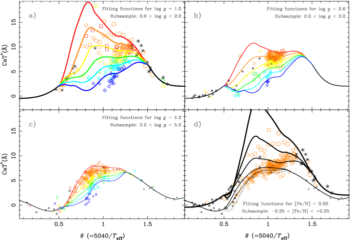
Figure 7: CaT^∗ values and general fitting functions for different atmospheric parameter regimes. Panels $a$, $b$ and $c$ display, respectively, all the stars with gravities in the ranges $0.0\leq\log g<2.0$, $2.0\leq\log g<3.2$ and $3.2\leq\log g<5.2$, together with the derived fitting functions for the mean gravity in each range, i.e., $\log g=$ 1.0 (a), 2.6 (b) and 4.2 (c). In the mid-temperature range, the different lines represent, from top to bottom, the functions for metallicities [Fe/H] = +0.5, 0.0, –0.5, –1.0, –1.5 and –2.0, whilst, for high and low temperatures, the fitting functions do not depend on metallicity. Panel $d$ shows all the stars around solar metallicity ($-0.25<{\rm[Fe/H]}\leq+0.25$) and the corresponding fitting functions computed for [Fe/H] = 0.0 and different values of gravity ($\log g$ = 0.0, 1.0, 2.0, 3.0, 4.0 and 5.0, from the thickest to the thinnest line). Codes and relative sizes of the star symbols (indicating, respectively, metallicity and gravity ranges) are explained in Fig. 3a. Note that, while the lines displayed here correspond to fitting functions at particular values of $\log g$ and [Fe/H], the plotted stars span a range of atmospheric parameters around these central values. This is the reason why the lines do not exactly fit all the points in the plots. Also, note that these fitting functions have not been derived by using only these plotted stars, but the whole sample.

As it is shown in Fig. 3c, the CaT^∗ index in hot stars ($0.13\la\theta\la 0.69$) shows a dichotomic trend for dwarfs on one side, and giants and supergiants on the other one. As a result of this, we designed boxes a and b in Fig. 6 (top) and derived different local fitting functions for the two groups of stars. Gravity effects are nearly negligible within each of the two luminosity bins. Also, due to the expected independence on metallicity for high temperature stars, only terms in $\theta$ were found to be statistically significant to reproduce the increasing CaT^∗ trend with decreasing temperature (Tables 4a and 4b). In the low temperature regime, the behaviour of cold dwarfs also differs from that of cold giants (Fig. 3c). Here, we followed the same strategy and derived two different local fits in which, again, only terms in $\theta$ were needed (Tables 4f and 4g). As we mentioned in Section 2.1, the decreasing CaT^∗ trend with increasing $\theta$ starts at lower temperatures for giants ($\theta\simeq 1.30$) than for dwarfs ($\theta\simeq 1.07$), being also steeper for the former group of stars. Finally, it is worth noting that, although a considerable number of hot and cold stars have unknown [Fe/H] determinations, the small scatter in the data shows that metallicity is indeed not governing the observed CaT^∗ behaviour at these temperature regimes.

The complex behaviour of warm and cool stars was parametrized in terms of the three atmospheric parameters (see Tables 4c, 4d and 4e). Although an unique parameter box enclosing the rest of stars was enough to reproduce the CaT^∗ behaviour at intermediate temperatures (box d in upper panel of Fig. 6), we designed transition boxes (c and e) at both sides to improve the quality of the interpolations with the local functions derived for hot and cold giants stars. Note that cold dwarfs follow a trend smoother than cold giants, and we did not need to include them in box d. Figures 7a, 7b and 7c illustrate the general fitting functions for three gravity bins (representing, roughly, supergiants, giants and dwarfs), showing an increasing dependence on metallicity as gravity decreases (therefore, supergiants span the widest range in CaT^∗ values). Figure 7d displays the derived fitting functions for solar metallicity and different gravity values. It is clear from this figure that gravity effects increase with decreasing gravity. Also, the higher the metallicity, the larger the gravity dependence. These effects were already apparent in Figs. 4 and 5.

Due to the lack of warm metal-poor giants (there are only a few stars in the sample), the local fit in Table 4c’ was specially designed to avoid unreliable interpolations between hot and warm giants in the low metallicity interval. Moreover, in order to ensure a smooth interpolation, the limits of this box are slightly different depending on the range of metallicity ($0.65<\theta<0.95$ for ${\rm[Fe/H]}\leq-1.25$, $0.65<\theta<0.90$ for $-1.25<{\rm[Fe/H]}\leq-0.75$, and $0.65<\theta<0.85$ for $-0.75<{\rm[Fe/H]}\leq-0.25$). Therefore, Fig. 6 only illustrates one particular case (dashed line).

It is important to note that, while the lines in Figure 7 correspond to projections of the fitting functions at particular values of $\log g$ and [Fe/H], the plotted stars span a range of atmospheric parameters around these central values. Therefore, it is not expected that the lines fit all the points in the plots. However, there are still some curves which do not appear to be well constrained by the observations in certain regions of the parameter space. For instance, there are no stars for $\theta<0.5$ in Figure 7a ($\log g=1.0$) and for $\theta>1.3$ in Figure 7b ($\log g=2.6$). Stars with these parameters do not exist (see Fig. 6), and therefore they will never be required by the stellar populations models. The curves at [Fe/H]$=+0.5$ (Figure 7a) and at $\log g=0.0$ (Figure 7d) for $0.50<\theta<1.0$ deserve a word of caution. The problem here is that high abundance, relatively hot supergiants are indeed rare and, therefore, uncertainties in the CaT^∗ predictions for this region may be present. Note that, since the fitting functions have been derived using the whole sample of stars within each parameter box, the CaT^∗ predictions for high metallicity, hot supergiants are partly driven by extrapolations of the functional dependence determined from stars of lower abundances and higher gravities. The contribution of this kind of stars (hot supergiants with metallicities above solar) at the near-IR spectra of old galaxies is not important, although it would not be the case for very young stellar populations.

3.2.2 PaT fitting functions

As in the case of the CaT^∗, the PaT index in hot and cold stars shows a different trend for dwarfs and giants. Once again, we designed proper boxes for each group (a, b, f and g in the lower panel of Fig. 6) and derived the local fitting functions given in Tables 6a, 6b, 6f and 6g. Figure 8 shows the general fitting functions for solar metallicity and different gravities. For hot stars, PaT increases as temperature decreases, reaching a maximum at a temperature that depends on the luminosity class. To reproduce the dependence on gravity of the hot dwarfs, a term in log g was deamed necessary. At the cold temperature end, the PaT in giant stars exhibits a bump due to the presence of strong TiO absorptions falling into the index bandpasses.

Warm stars follow a decreasing trend with increasing $\theta$ up to the cool stars which, as expected, attain values around zero. Boxes c and d were mainly designed to reproduce the maximum and the above trends. For cool stars, we have found a mild metallicity dependence in the sense that the larger the metallicity the stronger the PaT. Finally, box e allows smooth interpolations with the coldest stars.

Figure 8: PaT values for all the stars around solar metallicity ($-0.25<{\rm[Fe/H]}\leq+0.25$). The curves correspond to general fitting functions computed for [Fe/H] = 0.0 and different values of gravity ($\log g$ = 0.0, 1.0, 2.0, 3.0, 4.0 and 5.0, from the thickest to the thinnest line). Codes and relative sizes of the star symbols (indicating, respectively, metallicity and gravity ranges) are explained in Fig. 3a.

3.3 Residuals and error analysis

Figure 9: Residuals of the derived fitting functions ($\Delta{\cal I}={\cal I}_{\rm obs}-{\cal I}_{\rm pred}$) against $\theta$. See Fig. 3a for symbol codes.

We define the residual of any star as the difference between the observed index and the one predicted by the fitting functions ($\Delta{\cal I}={\cal I}_{\rm obs}-{\cal I}_{\rm pred}$). Figure 9 shows the residuals of the indices CaT^∗, PaT and CaT for the whole stellar library as a function of $\theta$. The residuals do not exhibit systematic trends with any of the three atmospheric parameters. Star clusters have also been analyzed separately and, except for the globular cluster M71, no systematic effects have been found. Compared to the predictions of the fitting functions, this cluster shows a significant mean offset of $\Delta{\rm CaT}^{*}=-0.35$ and $\Delta{\rm CaT}=-0.51$. The most plausible source of these systematic offsets is an error in the atmospheric parameters. A systematic error in the controversial reddening of this cluster would affect the adopted values. However, given the Ca ii triplet dependence on atmospheric parameters in this region of the parameters space, only a change in the adopted metallicity could account for the derived offsets. The controversy about the metallicity of M71 has already been discussed in Section 6.1 of Paper II. In fact, these residuals were used as one of the arguments in favour of the Carretta & Gratton (1997) metallicity scale (note that the value of ${\rm[Fe/H]}=-0.56$ established by the Zinn & West (1984) scale leads to even larger residuals). According to the predictions of the new fitting functions, M71 should have a metallicity of [Fe/H]$=-0.84\pm 0.06$, instead of the adopted value of ${\rm[Fe/H]}=-0.70$. Nevertheless, we have decided not to change the input metallicity of this cluster, keeping the Carreta & Gratton scale for all the globular clusters. Note that the CaT metallicity dependence is constrained by using more than 500 field and cluster stars, and a change in the adopted metallicity of M71 would not significantly alter the results. An anomalous [Ca/Fe] abundance ratio for M71 could also explain the derived offsets. However, using the tabulated data from Thévenin (1998), we derive a mean [Ca/Fe] ratio for this cluster of $0.28\pm 0.07$, which is significantly above the expected mean [Ca/Fe] value (0.13) for the cluster metallicity (see Figure 10) and, therefore, can not explain negative residuals in the indices.

Table 7: Statistical data for the general fitting functions of the indices CaT^∗, PaT and CaT. $\sigma_{\rm std}$: unbiased residual standard deviation; $\sigma_{\rm typ}$: typical index error for the stars used in the fits; $r^{2}$: determination coefficient.

	$\sigma_{\rm std}$	$\sigma_{\rm typ}$	$r^{2}$
CaT∗	0.534	0.184	0.965
PaT	0.427	0.163	0.965
CaT	0.629	0.197	0.939

Table 8: Uncertainties of the CaT^∗ fitting functions for different groups of stars, and mean CaT^∗ errors due to uncertainties in the input atmospheric parameters. $N$: number of stars. $\sigma_{\rm std}$: unbiased residual standard deviation of the fit. $\sigma_{\rm typ}$: typical observational CaT^∗ error for the subsample of stars. $\sigma_{\rm res}$: residual error (derived as $\sqrt{\sigma_{\rm std}^{2}-\sigma_{\rm typ}^{2}}$). $\sigma_{T_{\rm eff}}$, $\sigma_{\log g}$ and $\sigma_{\rm[Fe/H]}$: mean CaT^∗ errors due to uncertainties in the input $T_{\rm eff}$, $\log g$ and [Fe/H]. $\sigma_{{\rm par}}$: total error due to atmospheric parameters (quadratic sum of the three previous errors).

	$N$		$\sigma_{\rm std}$	$\sigma_{\rm typ}$	$\sigma_{\rm res}$		$\sigma_{T_{\rm eff}}$	$\sigma_{\log g}$	$\sigma_{\rm[Fe/H]}$	$\sigma_{{\rm par}}$
Open clusters (Coma, Hyades, M67, NGC188, NGC7789)	93		0.54	0.28	0.46		0.24	0.07	0.42	0.49
Globular clusters (M3, M5, M10, M13, M71, M92, NGC6171)	52		0.84	0.76	0.36		0.08	0.11	0.54	0.56
Field dwarfs	243		0.45	0.18	0.41		0.23	0.15	0.23	0.36
Field giants	201		0.46	0.16	0.43		0.15	0.26	0.23	0.38
Field supergiants	75		0.84	0.17	0.82		0.47	0.46	0.52	0.84
Hot stars ($0.13<\theta<0.69$)	68		0.66	0.17	0.64		0.81	0.23	0.42	0.94
Intermediate stars ($0.69<\theta<1.30$)	555		0.48	0.19	0.45		0.12	0.19	0.31	0.38
Cold stars ($1.30<\theta<1.84$)	41		0.71	0.14	0.70		0.69	0.20	0.21	0.75
All	664		0.53	0.18	0.50		0.22	0.20	0.31	0.43

In order to explore in more detail the reliability of the present fitting functions, in Table 7 we list the unbiased residual standard deviation from the fits, $\sigma_{\rm std}$, the typical error in the measured indices, $\sigma_{\rm typ}$, and the determination coefficient, $r^{2}$, for the 664 stars employed in the computation of the general fitting functions (note that, apart from the 23 stars listed in Table 3, 19 stars with unknown [Fe/H] could not be included in the metallicity-dependent fits). It is clear that, for the three indices, the computed $\sigma_{\rm std}$ is larger than what it should be expected uniquely from index uncertainties (see also the partial values of $\sigma_{\rm std}$ and $\sigma_{\rm typ}$ in Tables 4 and 6). Since we are confident that the latter errors are reliable (see full details on index errors computation in Section 5 of Paper I), the residuals must be dominated by a different error source. In fact, such an additional scatter could be due to uncertainties in the input atmospheric parameters of the library stars. In order to check this, we have computed how the parameters errors translate into uncertainties in the predicted CaT^∗. This depends both on the local functional form of the fitting function (e.g., a weak dependence on temperature leads to small index errors due to $T_{\rm eff}$ uncertainties) and on the atmospheric parameters range (e.g., hot stars have $T_{\rm eff}$ uncertainties larger than cooler stars). Thus, we have carried out the following analysis for different groups of stars (listed in Table 8).

For each star of the sample we have derived three CaT^∗ errors, arising from the corresponding uncertainties in $T_{\rm eff}$, $\log g$ and [Fe/H]. As input atmospheric parameters uncertainties we have made use of the values presented in Table 7 of Paper II. Apart from those, we have used errors of 75 K, 0.40 dex and 0.15 dex for the effective temperatures, gravities and metallicities taken from Soubiran, Katz & Cayrel (1998) (stars coded skc in Table 6 of Paper II), and 75 K, 0.05 dex and 0.20 dex for the cluster stars. For each star group we have computed a mean CaT^∗ error as a result of the uncertainty of each parameter ($\sigma_{T_{\rm eff}}$, $\sigma_{\log g}$ and $\sigma_{\rm[Fe/H]}$) by using the input parameters errors for all the individual stars. Finally, an estimate of the total expected error due to atmospheric parameters ($\sigma_{{\rm par}}$) is computed as the quadratic sum of the three previous errors.

Table 8 presents a comparison of these expected errors with the unexplained residual errors of the fits ($\sigma_{\rm res}\equiv\sqrt{\sigma_{\rm std}^{2}-\sigma_{\rm typ}^{2}}$). It is clear from this table that, in most cases, the additional scatter ($\sigma_{\rm res}$) is comparable to $\sigma_{{\rm par}}$, that is, it can be explained from uncertainties in the input atmospheric parameters. Using an $F$ test of comparison of variances we have checked that $\sigma_{\rm res}$ is not significantly larger than $\sigma_{\rm par}$, except for the intermediate stars. This means that, a minor, additional error source may still be needed to account for the observed residuals of field dwarfs and giants with intermediate temperatures.

Table 9: Absolute errors in the fitting functions predictions for different values of the atmospheric parameters. Input $\log g$ values varying with effective temperature for dwarfs, giants and supergiants have been taken from Lang (1991). Since, for extreme temperatures, the fitting functions do not depend on metallicity, no [Fe/H] value has been adopted for 15000 K and 3200 K. This is also the case for some values at 3500 K.

		dwarfs			giants			supergiants
$T_{\rm eff}$	[Fe/H]	$\Delta$CaT*	$\Delta$PaT	$\Delta$CaT	$\Delta$CaT*	$\Delta$PaT	$\Delta$CaT	$\Delta$CaT*	$\Delta$PaT	$\Delta$CaT
15000		0.17	0.25	0.29	0.17	0.25	0.29	0.24	0.60	0.61
8000	+0.5	0.39	0.29	0.47	0.45	0.25	0.51	0.60	0.32	0.67
8000	0.0	0.28	0.24	0.36	0.30	0.20	0.36	0.29	0.28	0.39
8000	–1.0	0.40	0.33	0.50	0.37	0.32	0.47	0.80	0.39	0.87
8000	–2.0	0.76	0.54	0.91	0.77	0.54	0.92	0.81	0.59	0.98
6000	+0.5	0.25	0.09	0.26	0.38	0.11	0.39	0.60	0.20	0.63
6000	0.0	0.10	0.06	0.11	0.22	0.09	0.23	0.37	0.20	0.41
6000	–1.0	0.17	0.09	0.19	0.34	0.11	0.35	0.50	0.21	0.54
6000	–2.0	0.37	0.16	0.40	0.58	0.18	0.60	0.68	0.25	0.72
5000	+0.5	0.28	0.07	0.29	0.19	0.04	0.20	0.31	0.08	0.32
5000	0.0	0.17	0.07	0.18	0.10	0.04	0.11	0.18	0.08	0.20
5000	–1.0	0.19	0.08	0.20	0.14	0.06	0.15	0.28	0.09	0.29
5000	–2.0	0.39	0.12	0.40	0.29	0.10	0.31	0.41	0.11	0.42
4000	+0.5	0.11	0.08	0.13	0.41	0.13	0.42	0.66	0.13	0.68
4000	0.0	0.11	0.07	0.13	0.26	0.12	0.28	0.54	0.12	0.55
4000	–1.0	0.11	0.07	0.13	0.38	0.13	0.40	0.40	0.13	0.42
4000	–2.0	0.11	0.10	0.15	0.74	0.16	0.75	0.54	0.16	0.56
3500	+0.5	0.13	0.10	0.16	0.97	0.19	0.98	0.99	0.19	1.00
3500	0.0	0.13	0.10	0.16	1.00	0.19	1.02	1.00	0.19	1.01
3500	–1.0	0.13	0.10	0.16	1.13	0.19	1.14	1.07	0.19	1.09
3500	–2.0	0.13	0.10	0.16	1.30	0.19	1.31	1.20	0.19	1.22
3200		0.19	0.13	0.23	0.37	0.22	0.42	0.37	0.22	0.42

Finally, since the aim of this paper is to predict reliable index values for any combination of input atmospheric parameters, we have also computed, making use of the covariance matrices of the fits, the random errors in such predictions. These uncertainties are given in Table 9 for some representative values of input parameters. Note that, as is expected, the absolute errors are larger for cold giants and supergiants and, in general, increase as the metallicity departs from the solar value.

3.4 Ca/Fe abundance ratios

Figure 10: [Ca/Fe] ratios against [Fe/H] for 216 stars of the library. Different symbols and sizes indicate metallicities and gravities as in Fig. 3a. The relationship ${\rm[Ca/Fe]}_{0}=0.013(\pm 0.012)-0.173(\pm 0.011)~{}{\rm[Fe/H]}$ (solid line) is a least-squares fit to the data and confirms an intrinsic anticorrelation between both abundance ratios.

Figure 11: Residuals of the CaT^∗ fitting functions (observed – predicted) versus residuals of the linear [Ca/Fe] relationship. Symbols and sizes for the 216 stars are as in Fig. 3a.

Since CaT^∗ is a pure Ca ii index, the parameter governing the metallicity dependence should be the actual [Ca/H] ratio, rather than the classical [Fe/H]. Since, in spite of this, we have been using [Fe/H] as our metallicity parameter, we have investigated whether the residuals of the CaT^∗ fitting functions are correlated with the individual Ca/Fe abundance ratios. Note that, if that were the case, this could account for part of the unexplained residuals reported in the previous section. Using a subsample of 216 library stars, for which we have compiled [Ca/Fe] data from the literature (Gratton & Sneden 1987; Pilachowski, Sneden & Kraft 1996; Nissen & Schuster 1997; Thévenin 1998), we have not found any evidence for such an expected correlation. This agrees with the results of ITD, which, after including a [Ca/Fe] term in their fitting functions, concluded that this relative abundance did not practically affect the value of CaT. In fact, a proper error analysis demonstrates that their derived [Ca/Fe] coefficient is not statistically different from zero.

To investigate this issue in more detail, in Figure 10 we plot the [Ca/Fe] relative abundances versus the assumed metallicities in [Fe/H]. As it has been previously reported (e.g. Edvardsson et al. 1993), there exists a clear anticorrelation between both abundance ratios for Galactic stars. A least-squares linear fit to all the stars in this plot gives ${\rm[Ca/Fe]}_{0}=0.013(\pm 0.012)-0.173(\pm 0.011)~{}{\rm[Fe/H]}$. The existence of this relation indicates that the actual calcium abundance has been implicitly taken into account in the fitting functions through the adopted [Fe/H] and, therefore, a systematic trend between the fitting functions residuals and the Ca/Fe ratios should not be expected. However we could still have a correlation between the residuals from the above relation ($\Delta{\rm[Ca/Fe]}={\rm[Ca/Fe]}-{\rm[Ca/Fe]}_{0}$), and the fitting functions residuals. Figure 11 shows that these residuals are not correlated at all. Thus, we conclude that the new fitting functions do not need any additional term to account for Ca overabundances within the library stars. Note however, that the fitting functions in their present form (i.e. using [Fe/H] as the metallicity indicator) implicitly include the chemical enrichment of the solar neighborhood, although, in principle, they could be corrected, by introducing a new [Ca/Fe]–[Fe/H] relation, to give predictions for other enrichment scenarios.

4 Comparison with previous fitting functions

In this section, we present a comparative analysis of the previous fitting functions by DTT, ITD and JCJ (see Section 2.2 and Table 2) and those presented in this paper. DTT and ITD made use of empirical stellar libraries of 106 and 67 stars repectively, and derived fitting functions for their calcium indices. On the other hand, using NLTE models, JCJ derived fitting functions for the theoretical equivalent widths of the Ca ii lines.

In order to avoid extrapolations of the previous fitting functions, the range of effective temperatures in which comparisons have been performed was constrained to the one approximately spanned by the three previous works ($0.75\leq\theta\leq 1.25$). Also, since the empirical papers by DTT and ITD do not correct for the Paschen contamination, their predictions are compared with our CaT fitting functions. For the comparison with JCJ we use the CaT^∗ fitting functions to compare with their theoretical Ca ii predictions, since they are based on model atmospheres which do not include the contamination by other elements.

Prior to any comparison, the previous fitting functions have been corrected from systematic offsets arising from differences in the index definitions. For the predictions by DTT and ITD, we have applied the calibrations given in Table 8 of Paper I, which were specially designed to convert the values of the literature indices to our system. Although JCJ do not define line-strength indices, they provide fitting functions for the total true equivalent width of the two strongest Ca ii lines. We have increased their predicted equivalent widths by 21.1($\pm 0.3$) percent. Such a fraction, which has been empirically derived using all the library stars within the range of effective temperatures given above, quantifies the strength of the weakest line of the triplet relative to the sum of the two other ones. Hence, after these corrections, differences between the predictions of the fitting functions will only arise from differences in the input data quality (in the case of the empirical papers, this will include the observational errors in the indices, the uncertainties in the atmospheric parameters and the number of calibrating stars), the range of atmospheric parameters spanned by the library, and the mathematical procedure to compute the fits.

Figure 12 shows the present Ca ii fitting functions (dashed lines) together with those derived by DTT, ITD and JCJ (solid lines). The predicted gravity effects are shown in the upper panels (a, b, c), whereas mid (d, e, f) and lower panels (g, h, i) show, respectively, the predicted dependences on metallicity for dwarf and giants.

DTT found a biparametrical, linear Ca ii behaviour with metallicity and gravity, but no dependence on temperature (see also the discussion in Section 2.2). Concerning the gravity effect, DTT predict a milder dependence than what our data shows, as it is apparent from Fig. 12a. Also, there are important differences at the other temperature ranges, although metallicity effects agree with our predictions, especially for warm dwarfs (Figs. 12d) and cool giants (Figs. 12g). We must note that most differences between DTT and our predictions arise from: i) the lack of second order and $\log g$–[Fe/H] cross-terms in their derived functions (a reanalysis of their data shows that these terms were indeed statistically significant), and ii) the absence of an effective temperature dependence. This last discrepancy is mainly due the lack of cold ($\theta>1.05$) dwarfs in their sample (see the effect in panel d) and to the contamination by Paschen lines (panel g).

The fitting functions by ITD include terms in effective temperature and several cross-terms in the parameters. They concluded that the gravity effect is not as important as the dependence on metallicity. Fig. 12b shows that their linear, extremely weak, gravity dependence, does not agree at all with our conclusions. As it was discussed in Section 2.2, this is mostly due to the scarcity of supergiants in their sample and to the fact that most of them have very low metallicities. On the other hand, the metallicity dependence for dwarfs and cool giants roughly matches with our predictions, although it is again very different for warm giants (Figs. 12e,h).

JCJ found a complex dependence on the three atmospheric parameters. Unlike the two previous empirical works, there is a good agreement between the qualitative behaviour of the parametrized gravity dependence (Fig. 12c), in the sense that the lower the gravity, the larger the gravity effect. Also, they find a metallicity dependence with a functional form similar to our predictions, although their values are more sensitive to metallicity than ours, especially for dwarfs (Figs. 12f,i).

We conclude that, in the temperature range of comparisons, the gravity dependence of the Ca ii triplet predicted by JCJ, rather than that of the empirical papers, roughly agrees with our results. On the other hand, for certain temperature ranges, DTT and ITD better reproduce the metallicity dependence found in this work.

Figure 12: Comparison with previous fitting functions. Panels a, b and c display, respectively, the predictions by DTT, ITD and JCJ for solar metallicity stars and different gravities ($\log g$ = 0.5, 1.5, 2.5, 3.5, and 4.5). The thicker the line, the lower the gravity. Solid lines correspond to the fitting functions by the above authors, whilst our predictions are given in dashed lines. Analogously, the predicted dependence on metallicity is also compared for dwarfs ($\log g=4.5$), in panels d, e and f, and giants ($\log g=2.5$), in panels g, h and i. The different lines represent, from top to bottom, the metallicities [Fe/H] = +0.5, 0.0, –0.5, –1.0, –1.5, and –2.0, for DTT and ITD, and [Fe/H] = +0.2, 0.0, –0.5, and –1.0 for JCJ. Note that, in all cases, the predictions by DTT and ITD are compared with the CaT fitting functions, whereas the theoretical work by JCJ is compared with CaT^∗.

5 Conclusions

In this paper, we have analysed the behaviour of the Ca ii triplet strength in the spectra of stars of different spectral types and luminosities, by means of a new near-IR stellar library (presented in Paper I) with a wide coverage of atmospheric parameters (Paper II). We have derived empirical fitting functions which can be easily implemented into stellar populations models. Readers interested in including these functions into their population synthesis codes can make use of the fortran subroutine referred to in Section 3.

Other results of this work are the following: i) We find a complex behaviour of the Ca ii strength as a function of the three main atmospheric parameters ($T_{\rm eff}$, $\log g$ and [Fe/H]). For hot and cold stars, effective temperature and luminosity class are the main driving parameters, whereas, in the mid-temperature regime, all three parameters play an important role (see Fig. 7). ii) The residuals of the fitting functions arise mainly from uncertainties in the input atmospheric parameters. iii) We do not find any correlation between these residuals and [Ca/Fe] abundance ratios. iv) A comparison with the fitting functions derived in the literature reveals striking differences in the predicted gravity and metallicity dependences for some regions of the parameter space (see Fig. 12).

Basically, compared to previous fitting functions for the Ca ii triplet, the main advantage of our predictions is that they include the whole range of effective temperatures. This is extremely important since the Ca ii behaviour in the temperature ranges explored by the previous works can not be extrapolated at all to hot ($\theta\la 0.75$) or cold stars ($\theta\ga 1.35$), as it is readily seen in, for instance, Fig. 3. We should not forget that these cold stars constitute a significant contribution to the integrated near-IR spectra of most stellar populations (to old populations through the role of cold dwarfs and giants, and to relatively young populations through the expected contribution of AGB stars; see Paper IV). This must indeed be remarked since, if the fitting functions by the previous works are extrapolated, stellar populations synthesis models will derive unreliable integrated Ca ii strengths which can not be compared with observations.

In the case of synthesis models that make use of the theoretical fitting functions of JCJ, the comparison of the predictions with the observed Ca ii triplet in galactic spectra is even more uncertain since: i) JCJ predictions do not include the contamination of Paschen lines, which affects the measurement of the observed index if the contribution of warm stars is not negligible; and ii) JCJ provides true equivalent widths, whereas line-strength indices in systems like that of DTT are used for the observational data. Although JCJ measure the strengths using the central bandpasses of DTT, these measurements can not be compared to indices in this system, since the local pseudo-continuum (traced between the sidebands) is far from being a true continuum (especially for hot and cold stars; see Paper I).

As a final conclusion, we want to emphasize the importance of using an empirical library with a wide range of accurate atmospheric parameters and a sufficiently large number of calibrating stars for deriving reliable empirical fitting functions. Also, well defined index definitions and objective fitting procedures are a critical factor. To summarize, the functions presented in this paper alleviate these problems and should lead to more reliable comparisons between models and observations than in the past. The first predictions of population synthesis models using these results will be presented in Paper IV.

References

- [Alloin 1989] Alloin D., Bica E., 1989, A&A 217, 57 (A&B)
- [Andrillat, Jaschek & Jaschek 1995] Andrillat Y., Jaschek C., Jaschek M., 1995, A&AS, 112, 475
- [] Bruzual G., Charlot S., 2001, in preparation
- [Carreta & Gratton 1997] Carretta E., Gratton R.G., 1997, A&AS, 121, 95
- [Carter 1986] Carter D., Visvanathan N., Pickles A.J., 1986, ApJ, 311, 637 (CVP)
- [Cenarro et al. 2001a] Cenarro A.J., Cardiel N., Gorgas J., Peletier R.F., Vazdekis A., Prada F., 2001a, MNRAS, in press (Paper I)
- [Cenarro et al. 2001b] Cenarro A.J., Gorgas J., Cardiel N., Pedraz S., Peletier R.F., Vazdekis A., 2001b, MNRAS, in press (Paper II)
- [Cohen 1978] Cohen J.G., 1978, ApJ, 221, 788
- [Díaz 1989] Díaz A.I., Terlevich E., Terlevich R., 1989, MNRAS, 239, 325 (DTT)
- [] Doyon R., Joseph R.D., Wright G.S., 1994, ApJ, 421, 101
- [] Edvardson B., Andersen J., Gustafsson B., Lambert D.L., Nissen P.E., Tomkin J., 1993, A&A, 275, 101
- [] Fioc M., Rocca-Volmerange B., 1997, A&A, 326, 950
- [García–Vargas 1998] García–Vargas M.L., Mollá M., Bressan A., 1998, A&AS, 130, 513
- [Gorgas et al. 1993] Gorgas J., Faber S.M., Burstein D., González J.J., Courteau S., Prosser C., 1993, ApJS, 86, 153
- [Gorgas et al. 1999] Gorgas J., Cardiel N., Pedraz S., González J.J., 1999, A&AS, 139, 29
- [Gratton & Sneden 1987] Gratton R. G., Sneden C., 1987, A&A 178, 179
- [Idiart 1997] Idiart T.P., Thévenin F., de Freitas Pacheco J.A., 1997, AJ, 113, 1066 (ITD)
- [Jones 1984] Jones J.E., Alloin D.M., Jones B.J.T., 1984, ApJ, 283, 457 (JAJ)
- [Jones 1995] Jones L. A., Worthey G., 1995, ApJ, 446, L31
- [Jørgensen 1992] Jørgensen U.G., Carlsson M., Johnson H.R., 1992, A&A, 254, 258 (JCJ)
- [Lang 1991] Lang K. R., 1991, Astrophysical Data: Planets and Stars, Ed. Springer-Verlag
- [] Leitherer C. et al., 1999, ApJS, 123, 3L
- [Mallik 1997] Mallik S.V., 1997, A&AS, 124, 359 (MAL)
- [Mallik 1994] Mallik S.V., 1994, A&AS, 103, 279
- [Mayya 1997] Mayya Y.D., 1997, ApJ, 482, L149
- [Molla 2000] Mollá M., García–Vargas M.L., 2000, A&A, 359, 18
- [] Nissen P.E., Schuster W.J., 1997, A&A, 326, 751
- [Pilachowski, Sneeden & Kraft 1996] Pilachowski C.A., Sneden C., Kraft R.P., 1996, AJ, 111, 1689
- [] Poggianti B.M., Barbaro G., 1997, A&A, 325, 1025
- [] Schiavon R.P., Barbuy B., Bruzual G., 2000, ApJ, 532, 453
- [Soubiran, Katz & Cayrel 1998] Soubiran C., Katz D., and Cayrel R., 1998, A&AS, 133, 221
- [] Tantalo R., Chiosi C., Bressan A., Fagotto F., 1996, A&A, 311, 361
- [Thévenin 1998] Thévenin F., 1998, Bull. Inf. CDS 49, Catalogue III/193
- [Vazdekis 1999] Vazdekis A., 1999, ApJ, 513, 224
- [Vazdekis et al.1996] Vazdekis A., Casuso E., Peletier R.F., Beckman J.E., 1996, ApJS, 106, 307
- [Vazdekis et al. 2001] Vazdekis A., Cenarro A.J., Gorgas J., Cardiel N., Peletier R.F., 2000, MNRAS, in preparation (Paper IV)
- [] Worthey G., Ottaviani D.L., 1997, ApJS, 111, 377
- [Worthey et al. 1994] Worthey G., Faber S.M., González J.J., Burstein D., 1994, ApJS, 94, 687
- [Zhou 1991] Zhou X., 1991, A&A 248, 367 (ZHO)
- [Zinn & West 1984] Zinn R., West M.J., 1984, ApJS, 55, 45