The Patchy Accretion Disc in HT Cassiopeiae

Abstract

We have reconstructed the temperatures and surface densities in the quiescent accretion disc in HT Cas by performing a Physical Parameter Eclipse Mapping analysis of archival UBVR observations. Using a simple hydrogen slab model and demanding a smooth, maximally artefact-free reconstruction, we derive a formal distance to HT Cas of $207\pm 10$ pc, significantly larger than the $133\pm 14$ pc we derive from a re-analysis of the data in the literature.

The accretion disc is small ($0.3-0.4~{}R_{\SS L1}$) and moderately optically thin but becomes nearly optically thick near the white dwarf. The temperatures and surface densities in the disc range from 9 500 K and 0.013 g cm^-2 in the center to about 4 000 K and 0.04 g cm^-2 at the disc edge. The mass-accretion rate in the disc is roughly constant but – at the derived distance – uncomfortably close to those which would prohibit the dwarf nova eruptions.

We argue that the larger derived distance is probably incorrect but is not produced by inaccuracies in our spectral model or optimization method. The discrepancy can be resolved if the emission regions on the disc are patchy with a filling factor of about 40% of the disc’s surface. This solves the problem with the high effective temperatures in the disc – reducing them to around 6 500 K within a radius of $0.2\,R_{\SS L1}$ – and reduces the derived temperature of the white dwarf and/or boundary layer from 22 600 to 15 500 K.

The viscosity parameters $\alpha$ derived from all reconstructed temperatures and surface densities are of order 10-100 and cannot be lowered significantly by invoking a lower distance or the filling factor. This situation is easily explained using the same patchy nature of the emitting material, since the quiescent disc cannot consist of optically thin regions alone, but also of a dark and hence cold and dense disc which could easily contain most of the matter. If we require global values of $\alpha$ of order 0.1, the implied total surface densities are 1-100 g cm^-2 – just like those expected for quiescent discs awaiting the next eruption.

We discuss several possible sources of the chromospheric emission and its patchiness, including irradiation of the disc, thermal instabilities, spiral-wave-like global structures, and magnetically active regions associated with dynamo action and/or Balbus-Hawley instabilities.

1 Introduction

Cataclysmic variables (CVs), are semi-detached binary stars consisting of a Roche lobe-filling late-type dwarf (the secondary star) which loses matter onto a white dwarf (the primary). Unless the primary has a considerable magnetic field, the transfered matter has enough specific angular momentum to create a gaseous accretion disc around this accreting star. Some CVs – the dwarf novae – have discs which occasionally have luminous phases of high mass-accretion but spend most of their time in a faint quiescent state. In quiescence, the optical light is usually dominated by optically thin line emission from the disc and continuum emission from the white dwarf, the disc and the bright spot caused by the impact of the transferred material onto the disc.

While spectral and eclipse observations of erupting dwarf novae show that the disc is optically thick during the outburst state, there is considerable uncertainty about the state of the quiescent discs. Theoretical models for the outbursts invoking a thermal instability as the cause of the eruption require that the quiescent disc store up material for the next eruption in a less viscous state in which the disc should be cool and optically thick (e.g. Ludwig et al. 1994). The inner disc may be emptied by irradiation from the hot white dwarf (Leach et al. 1999) or by a siphon flow fueled by a hot corona in the inner disc (Meyer & Meyer-Hofmeister 1994). Thus, the expectation is that the outer disc is cool and optically thick and the inner disc is warm/hot and optically thin.

HT Cas was once called “the Rosetta Stone of dwarf novae”, because – being one of the relatively few eclipsing dwarf novae – it more readily revealed its secrets (Patterson 1981). It has seldom been caught in outburst because of the unusually long outburst period of about 400 $\pm$ 50 days (Wenzel 1987). The quiescent periods may even last up to almost 9 years indicating an extremely low mass accretion rate in quiescence. The accretion disc is hardly visible during quiescence and the bright spot, the impact region of the accretion stream from the secondary, is nearly absent (Wood, Horne & Vennes et al. 1992, hereafter WHV92). The light curves predominantly show the eclipse of the white dwarf. The optical spectrum of HT Cas (Young, Schneider & Shectman 1981) shows double peaked emission lines of H I, He I, He II and Ca II, typical for a high inclination system ($i=81^{\circ}$: Horne, Wood & Stiening 1991, hereafter HWS91). Consistent with the broad-band photometry, the averaged profiles do not show any significant blue/red asymmetry, which would normally be attributed to the bright spot.

WHV92 investigated the accretion disc using multicolour eclipse photometry from which the contribution of the white dwarf had been subtracted. They produced independent classical eclipse maps for each colour and then modeled them with a two-parameter model spectrum yielding the temperature and surface density distribution in the disc. While this analysis suggested that the disc is optically thin – as expected – it suffers in detail due to the individual smearing of each eclipse map (see Vrielmann, Horne & Hessman 1999; hereafter VHH99). Furthermore, the pre-subtraction of the white dwarf contribution and the use of simple Cartesian reconstruction maps can make it difficult to produce a consistent physical picture of the various components.

Figure 1: The averaged quiescent light curves in UBVR together with the fits made simultaneously in all four filters. The contact phases of the white dwarf as given by Wood, Horne & Vennes (1992) are drawn as vertical dashed lines. The light curves are offset by 1.5 mJy, the horizontal dotted lines give the zero level for each light curve. In relation to this, the uneclipsed components and the residuals are plotted (solid lines).

Our present investigation is aimed at improving our understanding of the physical state of the quiescent accretion disc in HT Cas. We apply the Physical Parameter Eclipse Mapping method (PPEM) – a distinctly different tomographic ansatz (VHH99) which also uses the Maximum-Entropy Method (MEM; Skilling & Bryan 1984) – to the same UBVR photometry and derive the white dwarf temperature and the disc structure by simultaneously fitting all available eclipse light curves.

2 The data and system parameters

Since the dataset has been previously published and analysed, details about the acquisition can be found in HWS91. The photometric data consist of 16 eclipses taken in September 1982 and November/December 1983 at the Palomar 60-inch telescope using the Stiening photometer which gathers data in four filters simultaneously. The previous outburst occured in March 1980 and the quiescence lasted until the super outburst in January 1985. HT Cas was therefore in the middle of a quiescence period.

The original data have a time resolution of 1 s. As can be seen in Fig. 1 in HWS91 the basic eclipse shape appears to be constant, we do not even see a distiguished difference between the 1982 and 1983 data. But the individual eclipses suffer heavily from flickering. We averaged all light curves in order to enhance any stable patterns and minimize all random features, like flickering. The averaged light curves were then phase-binned to $\Delta\varphi=0.0015$ near the eclipse (within phases $-0.07$ and 0.07) and $\Delta\varphi=0.003$ outside this range (Fig. 1).

We used the photometric system parameters as given by HWS91, namely a mass ratio $q={\cal M}_{rd}/{\cal M}_{wd}=0.15$, an inclination angle $i=81^{\circ}$, as well as a white dwarf mass and radius of ${\cal M}_{wd}=0.61{\cal M}_{\odot}$ and $R_{wd}=0.0118{\cal R}_{\odot}=0.0263R_{\SS L1}$. With an orbital period of 106 min, the distance $R_{L_{1}}$ from the primary to the L₁-point is $3.13\times 10^{10}$ cm. The mass and radius of the secondary star derived by HWS91 are $0.09\,{\cal M}_{\odot}$ and $0.154\,{\cal R}_{\odot}$.

WHV92 determined the $E(B-V)$ as definately smaller than 0.2 and more likely between 0 and 0.1. Therefore, we neglect the interstellar reddening for our calculations.

3 Distance estimates

Wood et al. (1995), using UBVR photometry of the white dwarf extracted from the eclipse light curve, derived a value of 165$\pm$10 pc. Marsh (1990) deduced a distance of 140$\pm$14 pc using the observed Na I and TiO absorption spectrum of the secondary and his own calibration of the TiO $\lambda\lambda 7165,7665$ band strengths, a surface brightness calibration for M giants (the Barnes-Evans relation; Barnes et al. 1978), and the radial velocity amplitude $K_{2}$. This derivation makes several assumptions about the nature of the secondary star. Marsh predicted a mid-eclipse infrared H magnitude of $14.9\pm 0.1$ for the secondary but Berriman et al. (1987) measured $15.7\pm 0.2$, indicating that the system may be farther away than 200 pc. Two months after the first infrared measurements, Berriman et al. measured a much brighter H magnitude of 14.5, apparently confirming Marsh’s distance, but this difference could have been due to an increase in the constribution from the uneclipsed component (e.g. the outer regions of the disc). Although Zhang et al. (1986) derived an even larger distance of 320 pc from their analysis of BVR light curves, this distance is undoubtably made too large by their assumption of pure blackbody emission from the disc and the lack of U-band data.

Marsh’s estimate depends on his identification of the M5.4 $\pm$ 0.03 spectrum (derived from his own calibration of the TiO band strengths), the secondary’s flux at mid-eclipse ($0.224\pm 0.01$ mJy at 7 500 Å), and the Barnes-Evans relation (the surface brightness of giant stars versus V-R colour); Barnes et al. (1978). Beuermann et al. (1999) have recalibrated the Barnes-Evans relations (surface brightness versus colour) for both giants and dwarfs and find that the relation for M5 dwarfs is about 0.12 mag fainter than that for giants. This effect implies a 5% decrease in Marsh’s distance estimate ($132\pm 13$ instead of $140\pm 14$ pc). Marsh’s spectral type depends upon the relative strengths of the TiO features at $\lambda\lambda 7165,7665$: the latter band is contaminated with weak OI emission, so that the $\lambda 7165/\lambda 7665$ ratio may be over-estimated, and the spectral type later than M5.4. Though, the type is probably not any later than M6, since the region around TiO $\lambda 7165$ does not show the multiple absorbtion features prominent for later types.

Weichhold & Beuermann (2000) and Beuermann (2000) have also constructed a TiO surface brightness relation which can be used for systems like HT Cas with severe veiling. Using Marsh’s M5.4 $\pm$ 0.3 spectral type and assuming $M_{rd}=0.09\,M_{\odot}$, the observed TiO flux at mid-eclipse and a 94% correction for the Roche flattening at phase 0.0 implies a distance of $135\pm 14$ pc, in agreement with our revision of Marsh’s estimate. If the spectral type is as late as M6, this number drops to 93 pc, since the flux of the TiO bands drops rapidly after M5.5.

One can reverse the calculation and compute the expected spectral type given the observed TiO flux and assumed distance of 165 pc (Wood et al. 1995): this results in a spectral type of M4.5. This would imply an increase in the $\lambda 7165/\lambda 7665$ ratio of 43% over that measured by Marsh (1990), a ratio which is already too large due to OI contamination. A spectral type as early as M2-M3 (corresponding to a distance of $\sim$200 pc) can be simply ruled out because it would require twice as much light at mid-eclipse as is available for the secondary and the residual disc. The only way to change these results – given that the constraints come from the unilluminated backside of the secondary star – is to decrease the strength of the TiO band by lowering the metalicity to at least $[M/H]\approx-1.0$ (to get a reduction of the band depth by a factor $(133/200)^{2}=44\%$). However, there is no evidence to date of any low-metalicity CV’s (see Beuermann et al. 1998). An earlier spectral type is also implausible due to the fact that there is weak evidence that the spectral types of secondary stars in CV’s have later – not earlier – spectral types than normal main-sequence stars (Beuermann et al. 1998).

We must conclude that Marsh’s observations clearly suggest a distance of $133\pm 14$ pc (weighted average of $132\pm 13$ and $135\pm 14$ pc). This result remains in conflict with the eclipse-mapping results of Wood et al. (1995). Given that the latter depends upon several assumptions about the visibility of the white dwarf and its temperature, and that the plausible corrections to our re-analysis of Marsh’s result tend to make the distance smaller, not larger, we feel that our revision of Marsh’s estimate is still more reliable. Still, given the uncertainties, it is possible that the distance is somewhat larger.

In principle, the PPEM method can provide us with an independent estimate of the distance, as previously shown by Vrielmann, Stiening & Offutt (2002) if a proper spectral model is used. The use of an improper distance produces characteristic features in the maps of the fitted quantities. In Appendix A we demonstrate that reliable distances can be found by maximizing the entropy of the fit (making the disk maps as simple as possible) at fixed $\chi^{2}$ (requiring a good fit to the lightcurves). When the wrong distance is used, the disk maps become more complicated, and the entropy accordingly becomes increasingly negative. The best distance is thus identified as that which maximizes the entropy (simplicity) of the disk maps. The determination of a self-consistent distance to HT Cas was hence one of the objectives of this study.

4 The PPEM analysis

We used the two-parameter spectral model described in VHH99 to map the temperature $T$ and surface density $\Sigma$ of the disc material. The assumed spectrum is that of a simple uniform slab,

$$I_{\nu}=B_{\nu}(T)(1-e^{-\tau_{\nu}/\cos i})$$ (1)

where $\tau_{\nu}=\rho\,\kappa_{\nu}\,2H$ is the optical depth, $\rho=\Sigma\,/\,2H$ is the mass-density, $H\approx c_{s}/\Omega_{Kepler}$ is the vertical scale height of the slab, here assumed to be the disc’s semi-thickness, $\kappa$ is the mass absorption coefficient, $c_{s}$ is the sound speed and $\Omega_{Kepler}$ the Keplerian angular velocity of the disc material.

Although we assume a very simple pure hydrogen slab in local thermodynamic equilibrium (LTE) with no line emission, the difficulty in computing accretion disc spectra and our ignorance of the true vertical structure of optically thick or thin discs makes this model still very useful as a means of distinguishing between optically thick and thin parts of the disc.

At the densities and temperatures considered here, LTE is a very good approximation. The assumption of pure hydrogen is quite adequate for hot or warm regions of the disc. For realistic slabs (i.e. including metals) at temperatures lower than about 6 300K, the opacity is still mostly provided by H^- and hydrogen bound-free emission but the total opacity is much higher due to the increase in the number of free electrons relative to a pure-hydrogen gas. Thus, our method severely underestimates the intensity emerging from cooler parts of the disc. If a certain flux is required, the algorithm will be forced to increase the fitted temperature (which increases the opacity in this range) and/or increase the surface density. Regions of the reconstructed disc with kinetic temperatures less than 6 300K will thus – in fact – have true temperatures and/or surface densities which are significantly lower than those reconstructed using our simple model. Fortunately, this effect will only be important in the least-constrained outer disc where our ability to reconstruct physical parameters is the worst anyway (due to the disappearance of the Balmer Jump and low intensities in the observed filters). We will see that our upper limits on the parameters in some regions are still physically useful.

For theoretical spectra with no line emission, the physical parameter maps derived from the UBVR magnitudes are similar no matter whether one convolves the spectra with the filter band-passes or uses the monochromatic fluxes at the mean wavelengths of the pass-bands (indeed in the latter case our numerical results are slightly better). This is due to the fact that the continuum is very flat (similar fluxes in all four passbands). The inclusion of emission lines would improve the sensitivity of the maps to the U-band fluxes and regions with substantial H$\alpha$, and hence to the optically thin parts of the disc. However, this effect goes in the same direction as that mentioned before for the continuum: these less realistic models have less flux in the filter pass-band and so require higher temperatures and surface densities.

Since HT Cas was in quiescence at the time of observations, we assumed a geometrically thin disc for our PPEM study – an assumption which we will later verify.

We model the white dwarf emission using theoretical white dwarf spectra and treat the star as a true spherical star which is occulted by the secondary, occults the accretion disc behind itself, and can be preset to be partially occulted by the accretion disc. Wood & Horne (1990) find that the white dwarf is not likely to be partially occulted, although they could not completely rule out a partial occultation of the white dwarf. Our reconstructions (Section 6.2) imply that the inner disc is optically thick and therefore would lead to an occulted “lower” hemisphere of the white dwarf. On the other hand, evaporation of the inner disc (Meyer & Meyer-Hofmeister 1994) could lead to a small hole in the accretion disc which, with our limited spatial resolution, would be difficult to detect even with PPEM. However, for the white dwarf to be completely visible, the hole must be larger than $r_{\mbox{\scriptsize hole}}=R_{wd}\tan i=6.3R_{wd}=0.17R_{\SS L1}$, which should be easily detectable in the reconstruction. Thus, following Wood & Horne (1990), we first chose a fully visible white dwarf but then also reconstructed the accretion disc using a partially white dwarf for comparison (see Appendix D).

We assume the white dwarf has a uniform temperature $T_{wd}$, with no limb darkening ($u=0$, Wood & Horne). Therefore, we use HWS91’s white dwarf radius of 0.0263$R_{\SS L1}$, which is derived for a vanishing limb-darkening coefficient. Since the mean wavelengths of the filter pass-band partly coincide with the absorption lines in the theoretical white dwarf spectra, we integrated these spectra over the photometric filter pass-band functions to derive the theoretical white dwarf flux. These were then used within PPEM to determine the white dwarf temperature.

The slow ellipsoidal variations of the secondary star during quiescence and over the small range of orbital phases considered is roughly $\sim$13% of the secondary’s flux (Marsh 1990): given that the secondary star contributes certainly no more than 10% of the light in the R-band and much less in the others, we neglect the variation in the contribution of the secondary over the limited phase range between -0.1 and 0.1 and treat the secondary’s light as simply part of the fitted uneclipsed component.

For our reconstructions we used a default map with medium blurring, as described in Appendix E.

Figure 2: The entropy of the reconstructions (a measure of smoothness) as a function of the assumed distance. For each trial distance the data were fitted with $\chi^{2}/N=2.5$ (triangles), 2.0 (squares) and 1.75 (circles). The dashed lines are parabolic fits to the data, they peak at 214 pc, 210 pc and 207 pc, respectively.

5 Reconstructions using the $d\sim 150$ pc estimates

We first attempted to obtain PPEM paramater maps of the disc in HT Cas using the short distances of $d=140-165$ pc estimated by Wood et al. (1995) and Marsh (1990).

Unlike the results of Wood et al., our reconstructions must fit all of the data simultaneously and so suffer less from additional arteficial spatial smearing. Using $d=165$ pc we see typical features in the maps arising when too small a distance was chosen (Appendix B): they show emission in two bright regions along an axis perpendicular to the binary axis with one of them showing a curiously hot pixel. This is the algorithm’s desperate attempt to preserve the width of the eclipse profiles while minimizing the emitting area. The reconstructed disc using $d\sim 150$ pc would simply produce too much emission if it were axially symmetric.

We could fit the data with a reduced $\chi^{2}/N$ of 2.5 using a distance of 165 pc, but the entropy of the solution is very low compared to the entropies of the maps corresponding to larger trial distances, i.e. there are more arteficial structures and poorer fits for $d\sim 150$ pc. Reconstructions using Marsh’s smaller distance are even worse.

Otherwise, the reconstructions show similar radial temperature, surface density and derived parameter profiles as Wood et al. (e.g. a flat 8 000 K temperature profile within 0.17$R_{\SS L1}$ except for a nearly optically thick arteficial spot with a temperature of 10 000 K) and a disc radius of 0.35$R_{\SS L1}$. The white dwarf is reconstructed with a temperature of about 19 300 K, close to Wood et al.’s $18\,700\pm 1\,800$ K. Note that this reconstruction contains disc temperatures which should be reliable (i.e. are larger than 6 300 K). The effective temperature is also close to expected values of about 7 000 K at small radii. The optical depths range between 0.1 to 0.2 except near the white dwarf, where they reache values of $\sim$0.7.

Figure 3: The reconstructed radial temperature (left) and surface density distribution (right) for a distance of 205pc. The dashed line at 0.25$R_{\SS L1}$ indicates that for larger radii the parameter values become ambiguous, the solid line marks the disc edge.

Figure 4: Azimuthally averaged temperature (left) and surface density (right) distributions with error bars according to an analysis of the T-$\Sigma$ parameter space.

6 Reconstructions including a fitted distance

Given the problems in the reconstructions for $d\sim 150$ pc estimates, we next attempted to find the distance to HT Cas by using the entropy information in the maps (Vrielmann et al. 2002).

We reconstructed the accretion disc maps for a set of trial distances and determined the entropy for a fixed $\chi^{2}/N$. The result is presented in Fig. 2. A parabolic fit to the function for $\chi^{2}=1.75$ peaks at 207 pc, a distance which is significantly larger than the previous estimates using the white dwarf or the secondary flux. As a confirmation for this value, in Appendix C we show the maps using a larger distance of 240 pc showing typical features of too large a trial distance used.

We estimated the error in the PPEM distance estimate by performing the test described in Appendix A using an arteficial disc with a dominant bright spot. The resulting distance is 2.5% larger than the original one. This translates into an error of at least $\pm$5 pc for our distance of 207 pc.

In the following Sections we present the maps and derived quantities using the distance of 205 pc which should effectively give the same results as 207 pc. We use this distance although it does not agree with previous estimates and although we do accept the smaller distance of 133 pc because – as we will explain in Section 7.2 – the maps do represent part of the real disc.

6.1 The light curves

Despite the simplicity of the hydrogen model, we find a very good fit to the eclipse light curve, as shown in Fig. 1 with a $\chi^{2}/N$ of 1.75. The residuals (at the bottom of the plot) show little correlation, apart from the flickering between phases 0.055 and 0.075. In the U filter, this looks like the re-appearance of a bright spot, but the light curves in the filters V and R rather suggest two flares at phases 0.055 and 0.07.

The residuals between the observed and fitted light curves are at most 5.6% throughout the eclipse (between phases -0.05 and 0.05), in general largest for the V light curve and smallest for U and B, i.e. the Balmer Jump is very well reconstructed. The larger residuals of the V and R light curves may be due to the lack of line emission in our model, particularly H$\alpha$. This is also compatible with the R light curve having slightly negative residuals in mid-eclipse.

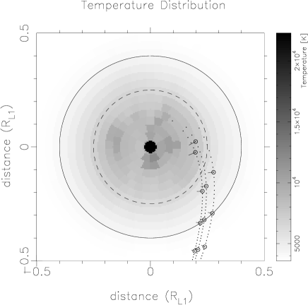
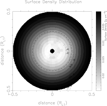
Figure 5: The reconstructed temperature (left) and surface density (right) map. The Roche-lobe of the primary component lies just about outside the plotted region. The dashed line at 0.25$R_{\SS L1}$ indicates that for larger radii the reconstructed parameter values become ambiguous, the solid line marks the disc edge. The curved, dotted lines in the grey-scale plot are theoretical accretion stream paths for mass ratios 0.15 $\pm$ 50%. The secondary is at the bottom.

6.2 The reconstructed accretion disc

The reconstructed temperature $T$ and surface density $\Sigma$ distributions (maps) are displayed in Fig. 4 and Fig. 5. The most prominent features are the radially decreasing temperature and increasing surface density. However, before reliable quantitative results can be drawn from these maps, the ($T,\Sigma$) parameter space has to be analysed in a way described in detail in VHH99.

This analysis shows that both the temperature and surface density values are very well constrained up to a radius of 0.25$R_{\SS L1}$. For radii larger than 0.25$R_{\SS L1}$, the fitted temperatures and surface densities become significantly anti-correlated and hence ambiguous. Since we reconstruct both parameters simultaneously, we cannot rely on the exact values of these two parameters for radii larger than 0.25$R_{\SS L1}$ and any derived parameters (with the exception of the effective temperature, see Section 6.5). To illustrate the reliability of the reconstructed values of $T$ and $\Sigma$, Fig. 4 shows azimuthally averaged parameter distributions with approximate error bars calculated using the assumption that the spectrum at each particular point may vary by up to a $\chi^{2}/N$ of 3. This $\chi^{2}/N$ is larger than that of the fit to the data and therefore allows some deviation of the parameters due to MEM smearing.

Given local values of temperature and surface density, we calculate the specific intensity distributions and find that the inner disc’s R-band intensity is 30% of that of the white dwarf. This drops with radius to 7% at 0.25 $R_{\SS L1}$, and to less then 1% at 0.4 $R_{\SS L1}$ which we call the disc edge. The region outside 0.25 $R_{\SS L1}$ contributes so little flux that the data provide only upper limits: the $T$ and $\Sigma$ values found in this range are controlled by the entropy extrapolating the radial $T$ and $\Sigma$ gradients defined by the data for the region inside 0.25 $R_{\SS L1}$.

The temperature in the inner part of the disc lies at about 9 500 K (with a range of 8 500 K to nearly 11 000 K) and drops to about 7 000 K at 0.25$R_{\SS L1}$ and to 4 000 K at the edge of the disc. The surface density increases in the same radial range from about 0.013 g cm^-2 to about 0.026 g cm^-2 at a radius of 0.25$R_{\SS L1}$ and 0.038 g cm^-2 at a radius of 0.4$R_{\SS L1}$. Given that the temperatures for $R>0.25R_{\SS L1}$ are lower than 6 300 K, – corresponding to temperatures where our spectral model is bound to underestimate both physical parameters – the true temperatures and/or surface densities are likely to be lower. Thus, we estimate that the outer disc radius is 0.3-0.4 $R_{\SS L1}$.

To obtain a bolometric measure of the optical depth, we compare the spectrally averaged intensity distribution $I(T,\Sigma)$ to the black body intensity distribution $I_{BB}(T)$ derived from the reconstructed temperature $T$ (Fig. 6). The ratios of the intensities at each radius show that all of the disc has an optical depth of order unity, but the inner parts are more nearly optically thick. A more quantitative picture is drawn by the spectra of different disc regions as shown in Fig. 7. The parameters are selected according to the azimuthally averaged maps (Fig. 4). While the Balmer Jump is present in the central parts, it disappears for radii larger than 0.25$R_{\SS L1}$, because of the low intensity at the blue end of the spectrum. Note that the disc is optically thin at all radii in the B-band, is marginally thin in the V-band, is optically thick in the inner disc in the U-band, and nearly optically thick in the R-band.

The leading side of the inner disc has higher optical depths and so is closer to a black-body radiator. This coincides with the larger temperature and surface density values seen in Fig. 4 at small radii. This asymmetry is reproduced in the eclipse profile of the accretion disc. To explain the asymmetry in the light curve, we seperate the phases in four different ranges $A,B,C,D$ with $A<\phi_{wd,i}$, $\phi_{wd,i}<B<0$, $0<C<\phi_{wd,e}$ and $\phi_{wd,e}<D$ where $\phi_{wd,i}$ and $\phi_{wd,e}$ denote the phases of white dwarf ingress and egress, respectively. Before the white dwarf is eclipsed, we see a gradual, linearly sloped disc ingress (phase range $A$). While the central star is obscured, the disc ingress profile is short and rounded, reaching minimum light before phase 0 ($B$). The following egress ($C$) is again more gradual and after the reappearance of the white dwarf we see the short, steep egress of the remaining disc ($D$). Phases $A$ and $C$ with the more gradual profiles correspond to the following lune, phases $B$ and $D$ to the leading, brighter lune of the accretion disc. Hence, the leading lune has a steeper gradient in the parameter distributions than the following lune. A comparison with a much more symmetric reconstruction of the disc corresponding to a fit to the data with $\chi^{2}/N=2.5$ shows that exactly these features in the eclipse profile are responsible for the asymmetric parameter distributions. At this higher $\chi^{2}/N$ level we see correlated residuals especially inside the white dwarf eclipse profile.

For comparison, we reconstructed the accretion disc using a partially visible white dwarf. The results are described in Appendix D. We note here only that considering the PPEM method, the solution with the partially visible white dwarf is inferiour to the above presented solution.

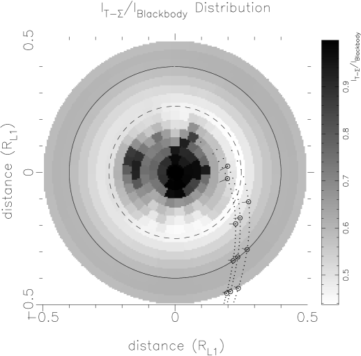
Figure 6: Left: The radial distributions of the spectrally and azimuthally averaged intensity distributions of $I(T,\Sigma)$ and $I_{BB}(T)$. Right: The distribution of the ratio $I_{T,\Sigma}/I_{BB}$ as a gray-scale plot (see text for explanation). The Roche-lobe of the primary component lies just about outside the plotted region. For both plots: The dashed line at 0.25$R_{\SS L1}$ indicates that for larger radii the reconstructed parameter values become ambiguous, the solid line marks the disc edge. The curved, dotted lines in the grey-scale plot are theoretical accretion stream paths for mass ratios 0.15 $\pm$ 50%. The secondary is at the bottom.

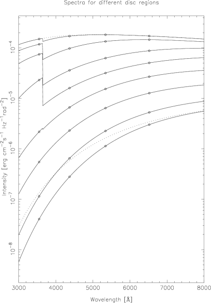
Figure 7: Reconstructed intensity spectra for disc radii 0.03 (uppermost), 0.08, 0.15, 0.22, 0.28, 0.35, 0.42 and 0.48 $R_{\SS L1}$ (lowermost) with overall intensity decreasing monotonically with increasing radius. The parameters $T,\Sigma$ used to calculate the spectra are the averaged values from Fig. 4. Additionally, black body spectra are shown for comparison at temperatures 9 900 K (upper dashed line) and 3 650 K (lower dashed line), corresponding to the inner and outer disc temperatures at 0.03 and 0.48 $R_{\SS L1}$, respectively; the circles indicate the mean wavelengths of the UBVR band-passes.

6.3 The white dwarf

Our white dwarf fluxes are 0.55 mJy, 0.51 mJy, 0.43 mJy and 0.31 mJy for the filters UBVR, respectively. Except for the U flux, our white dwarf fluxes are smaller than WHS’s fluxes (their Table 1). The remaining flux in the BVR filters must originate in the inner part of the accretion disc.

The reconstructed temperature of the white dwarf is 22 600 K. This value is larger than Wood et al.’s (1995) value of $18\,700\pm 1\,800$ K determined from the same data, because of the larger distance used. If we use a partially obscured white dwarf (Appendix D) we arrive at a white dwarf temperature of $T_{wd,1/4}=26\,700$K, even larger than Wood et al.’s (1995) value.

The fact that PPEM favours a fully visible white dwarf is problematic, because this means we should expect a substantial hole in the inner part of the disc of the radial size $0.17R_{\SS L1}$. Such a hole is not evident in our reconstructions. However, Wood & Horne’s (1990) analysis of the white dwarf ingress and egress profiles also favours a fully visible white dwarf or a white dwarf fully covered by a boundary layer, but specifically excludes a white dwarf with $u=0$ and an occulted lower hemisphere.

In our study we have not specified a location of boundary layer, but expected it to be reconstructed in the inner disc. Since we do not see any indication of a boundary layer in the disc, its temperature must be mixed into the white dwarf temperature, making it in our model indistinguishable from the central object. In this scenario might lie the solution to the problem, since the boundary layer has a different geometrical and radiative structure than a white dwarf.

The white dwarf or boundary layer appears to have different temperatures at different times, as reported by Wood et al. (1995): it varies between 13 000 and 20 000 K, lower temperatures associated with low states of the accretion disc. The white dwarf and/or boundary layer cools down during quiescence when the accretion rate is reduced and is heated up again during an outburst. Since the HT Cas data were taken 2-3 years after the previous outburst, the temperatures derived using $d\sim 200$ pc would appear to be too high compared with those of white dwarfs in similar dwarf novae. However, the current mean mass-accretion rate does not necessarily reflect the long-term rate, so that high temperatures could principally be due to a previous phase of high mass-accretion rates (e.g. Schreiber, Gänsicke & Cannizzo 2000).

6.4 The uneclipsed component

Figure 8: The uneclipsed component (dashed line) in comparison to the mideclipse flux (solid line) and the contribution of a M5.4 dwarf star at a distance of 133 pc (dash-dotted line) and at 207 pc (dotted line). The points with error bars give a mean and standard deviation of the uneclipsed flux for reconstructions with three different default maps (little, medium and much, see Appendix E) to illustrate the uncertaincy of the reconstructed value.

Table 1: The reconstructed fluxes in mJy of the uneclipsed component ($F_{\mbox{\scriptsize un}}$), the total mid-eclipse fluxes ($F_{\mbox{\scriptsize mid}}$), and the the total out-of-eclipse fluxes $F_{\mbox{\scriptsize out}}$ compared with the flux of an M5.4 main sequence star at 133 and 207 pc ($F({\mbox{\scriptsize M5.4}})$). Columns 5 and 6 give the mean and standard deviation of the uneclipsed flux for reconstructions with three different default maps (little, medium and much, see Appendix E) to illustrate the uncertaincy of the reconstructed value.

Filter	$F_{\mbox{\scriptsize out}}$	$F_{\mbox{\scriptsize mid}}$	$F_{\mbox{\scriptsize un}}$	$<F_{\mbox{\scriptsize un}}>$	$\sigma(<F_{\mbox{\scriptsize un}}>)$	$F_{\mbox{\scriptsize M5.4}(133)}$	$F_{\mbox{\scriptsize M5.4}(207)}$
U	1.13	0.127	0.099	0.106	0.002	–	–
B	0.98	0.104	0.078	0.075	0.003	–	–
V	1.00	0.103	0.018	0.010	0.011	0.021	0.009
R	1.20	0.231	0.124	0.082	0.028	0.095	0.039

The uneclipsed component is the fitted flux in each band-pass which does not appear to be eclipsed and includes the contribution of the secondary star. The uneclipsed component comprises no more than 8-10% of the total. It increases to the UV, indicating a hot uneclipsed source like a chromosphere above the disc (Fig. 8), reaching so far above the disc that it is never eclipsed (i.e. a few white dwarf radii).

Assuming an M5.4 main sequence star (Marsh 1990) and using the Kirkpatrick & McCarthy (1994) flux tables, we can estimate the contribution of the secondary star to the uneclipsed component (Tab. 1). All the uneclipsed light in V and R can be accounted for if we assume the smaller distance of 133 pc to be the correct one (see Tab. 1). The fact that actually the expected V and R fluxes are somewhat higher than the reconstructed one in this case is due to the uncertainty in the determination of the uneclipsed flux. However, it could also indicate that the secondary is more likely of slightly later type, a suggestion mentioned in Section 3. Alternatively, the hot uneclipsed source is bound to have some V and R flux, a situation easily accounted for in the solution with the larger PPEM distance in which the secondary contributes less light.

Figure 9: The radial effective temperature distribution for a distance of 205 pc (circles) and 133 pc (dots) assuming a covering factor of 41%. The underlying dotted lines are theoretical steady state temperature distributions for $\log\dot{\cal M}=13$ to 18, the one for $\dot{\cal M}=10^{16}$gs^-1 is drawn solid for reference. The dashed-dotted line indicates the critical mass accretion rates $\dot{M}_{\rm A}$ according to Ludwig et al. (1994). The vertical dashed line at 0.25$R_{\SS L1}$ indicates the radius above which the reconstructed parameter values become ambiguous. The vertical solid line marks the disc edge.

6.5 Derived parameters

The reconstructed T-$\Sigma$-maps allow us to derive further parameters like the effective temperature or mass-accretion rate distribution, the apparent viscosity, and the disc height and mass.

The effective temperature $T_{\mbox{\scriptsize eff}}$

The effective temperature is calculated as the integral of the intensity of the emission over all directions $\Omega$ and frequencies $\nu$

$$\int\!\!\!\int I_{\nu}(T,\Sigma)\,\,d\nu\,\,d\Omega=\sigma T_{\mbox{\scriptsize eff}}^{4}$$ (2)

with $\sigma$ the Stefan-Boltzmann constant and $I_{\nu}$ according to Eq. 1.

Fig. 9 shows the effective temperature distribution calculated directly from our spectral model and the fitted parameters. Even though the reconstructed parameters $T$ and $\Sigma$ are somewhat ambiguous for radii larger than $0.25R_{\SS L1}$, the effective temperature $T_{\mbox{\scriptsize eff}}$ is reasonably reliable, since I($T$, $\Sigma$) must still be reproduced (the light curves are fitted very well) and the optical flux is a large fraction of the bolometric flux.

Within a radius of 0.2$R_{\SS L1}$ the $T_{\mbox{\scriptsize eff}}$ distribution is relatively flat, with values around 7 500 K or 10 000 K. The distribution of $T_{\mbox{\scriptsize eff}}$ is distinctly spatially separated, following the pattern of the optical depth (with higher $T_{\mbox{\scriptsize eff}}$’s corresponding to the optically thick and lower $T_{\mbox{\scriptsize eff}}$’s to optically thin regions). For radii larger than 0.2$R_{\SS L1}$, the disc appears to be compatible with a steady state disc with a mass accretion rate around $3\times 10^{15}$gs^-1 (i.e. $5\times 10^{-11}{\cal M}_{\odot}\!\mbox{yr}^{-1}$).

Also shown in Fig. 9 is the critical effective temperatures as a function of radius predicted by Ludwig et al. (1994). This corresponds to the critial mass-accretion rates above which we would expect steady accretion in an optically thick disc to occur. Within a radius of 0.2$R_{\SS L1}$ our derived $T_{\mbox{\scriptsize eff}}$ lie above this line. Since the data were taken in the middle of a quiescent period, the effective temperatures should not have reached above the critical values.

The viscosity

The most important parameter describing the disc is the viscosity $\nu$, usually parametrizised as $\nu=\alpha c_{s}H$ (where $c_{s}$ is the local sound speed and $H$ the disc scale height) using the Shakura & Sunyaev (1973) $\alpha$-parameter. In order to be able to fit the dwarf nova light curves with current accretion disc models, we need values of $\alpha$ around 0.01 in quiescence (e.g. Smak 1984).

Using the standard relation between the viscously dissipated and total radiated flux $F_{\nu}=I_{\nu}d\Omega$,

$$2H\alpha P\frac{3}{4}\Omega_{K}=\int_{0}^{\infty}F_{\nu}d\nu=\sigma T_{\mbox{\scriptsize eff}}^{4}$$ (3)

where $P$ is the (gas) pressure, we can map the viscosity parameter $\alpha$ of the disc material. The derived values lie between 20 and 230, far larger than those expected in any kind of turbulent accretion disc and similar to those derived by WHV92.

The disc height and mass

The equilibrium disc height ratio, $H/R=c_{s}/\Omega_{\mbox{\scriptsize K}}$ ($c_{s}$ is the local sound speed and $\Omega_{\mbox{\scriptsize K}}$ the Keplerian angular velocity of the disc material) is roughly 0.01, i.e. the disc has a very small opening angle of a degree or less. The innermost part of the disc and the disc towards the edge are even narrower (with an opening angle of approximately $0^{\circ}_{\raisebox{1.80835pt}{\hskip 0.35002pt.}}4$) giving the disc a slightly concave shape in the inner region and convex shape in the outer part. In any case, the reconstructed disc is extremely thin, justifying (at least internally) our thin disc approximation.

Within a radius of 0.4$R_{\SS L1}$ the mass of the disc is $5.4\times 10^{19}$ g ($2.7\times 10^{-14}{\cal M}_{\odot}$). This factor is uncertain by up to 50% due to the ambiguity of the surface density density values in the outer parts. A more robust calculation of the disc mass for the inner part of the disc (up to a radius of 0.25$R_{\SS L1}$) leads to $1.3\times 10^{19}$ g ($6.4\times 10^{-15}{\cal M}_{\odot}$).

7 The resolution of the discrepancy

Our PPEM distance of 207 pc is significantly larger than the estimates of $140\pm 14$ pc by Marsh (1990), $165\pm 10$ pc by Wood et al. (1995) and our revised estimate of $133\pm 14$ pc from Section 3. The main problem with the reconstructions using $d\sim 150$ pc is the appearance of characteristic distortions due to too much flux from the nearer disc, a problem which can easily be remedied by increasing the distance. On the other hand, the PPEM reconstructions at $d\sim 200$ pc also have their problems, notably effective temperatures, $T_{\mbox{\scriptsize eff}}$, which are higher than those expected for quiescent discs. Both solutions suffer from the fact that the values of the viscosity paratmers, $\alpha$ are orders of magnitude higher than can be physically explained.

We therefore need to check quite critically the potential pit-falls in our own analysis and – if the method can be shown to be reliable enough – to explain the behaviors of the different reconstructions using an improved physical model of the disc.

7.1 Reliability of the PPEM method

If our reconstructions would like to have a distance which is too high, we must identify which false assumption has produced this result. There are several possible explanations for the discrepancy.

• This effect could be a peculiar side-effect of the PPEM approach since it did not show up in classical eclipse mapping analyses. However, the latter do not use the constraints on the colors and spectral shapes of the mapped regions and are thus free to yield even very unphysical solutions. The simultaneous use of all the information as well as the physical constraints posed by the physical (if simple) spectral model should make PPEM more sensitive to such effects. Thus, it is not surprising that this problem did not arise in WHV92s analysis and there is no a priori reason why PPEM should not produce reasonable results.

• Wood et al.’s distance is based on the white dwarf colours alone, which were deduced from the original eclipse light curve while our analysis includes the information of the accretion disc. Furthermore, the distance Wood et al. fitted is not independent from the temperature fitted to the white dwarf fluxes. We believe our method is therefore more advantageous.

• As we have explained, our model for the emission from the disc does not necessarily describe the true emissivity of the disc, both because we have no a priori knowledge of the structure of the disc and because of our use of pure hydrogen spectra. However, the reason that our algorithm produces a larger distance is that the surface brightness of the disc is basically set by the colours and the eclipse width, which, for a given orbital separation, corresponds to a maximum size of the emitting region. Solutions with smaller distances have disc fluxes which are too large for the given spectra and areas, i.e. the specific intensity of the disc would have to be smaller. Lowering the surface density would decrease the intensities, but also changes the colours, since this would produce a large change in the optically thinnest part of the spectrum. The algorithm therefore reacts by reconstructing a disc with much more scatter, i.e. a much smaller entropy and a more or less elliptically shaped emission region with the long axis perpendicular to the binary axis. This is an unphysical response to a physically constrained but primarily numerical problem. Our assumption of pure hydrogen spectra already underestimates – not overestimates – the intensities from the cooler outer disc. Thus, we expect that the use of improved spectral models would not necessarily solve this distance problem.

• The distance could also be affected by our assumption of a pure hydrogen spectral model neglecting any line emission from hydrogen and other elements. While it is formally not difficult to include the lines, the theoretical line fluxes are more dependent upon the detailed model of the vertical structure of the disc, are principally more sensitive to the diffuse outer layers of the emission region which do not contribute much to the total optical depth, and suffer from direction-dependent opacity effects due to the shear in the disc (Horne & Marsh 1986). Only a test with an apropriatly complicated model would clarify this; in a future paper we will use more realistic disc spectra calculated with models from Hubeny (1991). A preliminary analysis is shown in Vrielmann, Still & Horne (2001). We previously noted, that when hydrogen dominates the continuum opacity and supplies most of the electrons, then metals have little effect on the spectrum. Only in cool disc regions will the metals have a noticable effect on the opacity. However, these regions have a low intensity. We therefore think that our assumption is acceptable and that the lines do not play a major role at the high densities implied by the reconstructed maps.

• Another assumption that might influence the distance estimate is our neglect of a dramatic vertical stratification of the disc. While the effect on the distance determination is also difficult to estimate and a full consideration lies beyond the scope of this paper, we consider a scenario in which the disc consists of a cool disc with a hot chromosphere. In this case, the main emission source is at the base of the chromosphere. Because chromospheres tend to stabilize around 10,000 K due to the strong dependence of opacity on temperature when hydrogen is ionized (Williams 1981, Tylenda 1981), our assumption should not be so bad.

• And finally, Vrielmann (2001) & Vrielmann et al. (2002) were able to determine a PPEM distance for UU Aqr and V2051 Oph that agree very well with previous estimates. Furthermore, they found no discrepancy to previous distance estimates for the systems IP Peg and VZ Scl. This gives us confidence in our method, though naturally, it must be tested on more systems.

As the method itself cannot clearly be blamed for the discrepancy, we must find another solution to this discrepancy tied to the structure of the disc itself.

7.2 The solution: a patchy disc

An attractive way to reduce the flux from the disc without substantially changing the colours and total disc area is by allowing for a covering factor: the disc need not be uniformly covered with emitting material if only a fraction of the local disc surface can produce the observed optical flux. Since the “chromospheric” emission modelled here is also seen in the near infrared in other quiescent dwarf novae (Berriman et al. 1985), the remaining area must be filled with “dark” material which may only show up at even longer infrared wavelengths, i.e. dark patches which are invisible in the optical part of the spectrum. The covering factor we require is about $C=(133/207)^{2}=41$%.

While the presence of such a covering factor $C<100\%$ is a plausible solution of the distance discrepancy, it is at present not possible to establish if and how the covering factor may change with disc radius or azimuth. In future analyses where the distance to a CV is well known one may consider adding a covering factor $C$ as an additional parameter to be mapped. This may be especially viable if we use eclipses of the line emission.

Fortunately, the physical parameters of the patchy disc located at the (true) $d\sim 150$ pc will not be very different from those reconstructed at $d\sim 200$ pc since the total subtended area of the emitting regions (as opposed to the total disc area) is the same. This preserves all of the important spectral properties except the effective temperatures, $T_{\mbox{\scriptsize eff}}$. The latter are derived from the bolometric fluxes and the total (rather than the emitting) areas; the $T_{\mbox{\scriptsize eff}}$’s need to be scaled down to match the lower distance by a factor of $(0.41)^{1/4}=$80%. The resulting mass-accretion rates in the maps are thereby lowered (as can be seen in Fig. 9) to values below or at least closer to the critical mass-accretion rate.

By moving HT Cas closer, the fitted temperature of the white dwarf is also reduced. In Appendix F we show a reconstruction with a fixed covering factor $C=41\%$ for a distance of 133pc. The resulting white dwarf temperature is 15 500 K. For 150 pc and $C=52\%$, we get 17 450 K, close to Wood et al.’s (1995) value of $18\,700\pm 1\,800$.

The $\alpha$ values will also be reduced for such a patchy disc, but only down to values of 10-100. However, the presence of additional but optically unseen material solves the problems associated with the still unreasonably large $\alpha$ values: if most of the viscous transport occurs in the unseen material and the small amount of observed “chromospheric” material finally radiates away this dissipated energy, then reasonable values of the “turbulent” viscosity can be invoked. The relative amount of unseen matter is then at least equal to the inverse of the derived $\alpha$, i.e., of the order of tens or hundreds of grams per cm². As theoretical calculations (e.g. Ludwig et al. 1994) show, the hysteresis curve in the effective temperature - surface density diagram used to explain dwarf nova outbursts lies just at these surface density values.

Thus, if at optical wavelengths we only see the chromosphere, we underestimate the surface densities severely and therefore overestimate the $\alpha$’s. A simple estimate shows that just such surface densities of 10-100 g cm^-2 in an underlying cool disc lead to the desired values of $\alpha<1$.

An analysis of single eclipses (see Fig. 1 in HWS91) could in principle reveal the pattern, however, the pattern would be smeared out due to the differential rotation of the disc. Another problem one encounters with mapping single eclipses is the flickering, easily hiding just such small steps expected in the eclipse profile. The flickering introduces features in the map that cannot be distinguished from real patterns of a patchy disc.

Our analysis therefore reveals the disc as an average between the bright and dark patches. If the dark patches are so cool that they are basically undetectable at the optical wavelength at which the data were taken, the spectra (colours) in the disc are determined by the bright patches. A time average, however, is lower in intensity than that of an active region, due to the averaging over times when the patch is present and absent. This leads to the increase in distance that we derive using PPEM.

8 The source of the patchiness

The PPEM reconstructions of the intensity distribution of the disc in HT Cas imply that the optical emission does not cover the entire face of the disc. If proven, this fact would place severe constraints on the implied structure of the disc. In this model, most matter is carried by an underlying optically thick, cool accretion disc which generates the energy finally radiated away in the chromosphere. This underlying disc must have surface densities of the order of tens to hundreds of g cm^-2 in quiescence in order to explain the dwarf nova eruptions (e.g. Ludwig et al. 1994).

The presence of patchiness would argue against models for chromospheric emission which is simply produced either by irradiation-induced coronae (Smak 1989) or thermally unstable viscous atmospheres (Adam et al. 1984), since these processes should produce a uniform chromospheric layer over the entire geometrically thin disc. This argument could be weakened if the disc were able to maintain a vertically “corregated” structure like that suggested in systems with spiral waves (Steeghs, Harlaftis & Horne 1997), in which case either irradiation or locally viscous and thermal processes could produce the required mottled emission. For example, the opening angle of spiral waves in discs is supposed to decrease with decreasing azimuthal Mach number, so quiescent discs may have very tightly wound-up spirals which either produce local dissipation or raise material high enough to be irradiated by the central disk/star.

An alternative model is that the patches are similar to active regions on the surface of the sun and could be linked to the flickering in the disc. These regions could be due to magnetic activity in localized regions on the surface or in the upper layers of the accretion disc. For example, magnetic flux created by dynamo action and/or the Balbous-Hawley instabilities driving the viscosity would rise out of the cool midplane regions and dissipate most of the viscously generated energy via magnetic reconnection or similar coronal processes. This model would also explain why the emission line intensities are proportional to the local orbital frequency (Horne & Saar 1991).

The previous models generally assume that the optical emission region is an upper layer above an optically invisible disc containing most of the mass, even locally along a vertical cut through the disc. A very different alternative is suggested by the observation of “mirror” line eclipses in the Paschen lines in the dwarf nova IP Peg by Littlefair et al. (2001) at orbital phases around 0.5. Such behavior can only be explained by having a disc which is optically thin enough to let the light of the secondary star shine partially through the disc at phase 0.5. This observation is inconsistent with a uniform, optically thick cold disc with surface patches of chromospheric emission on top (and bottom) and suggests (1) that the patches implied by the PPEM reconstructions are exactly those areas of the disc which are vertically truly optically thin and (2) that the dense, cold material needed to explain both the surface densities necessary to explain the dwarf nova eruptions and the anomalous derived viscosity parameters is laterally rather than vertically distinct from the chromospheric patches. The fact that the “mirror” eclipses are seen at large Keplerian velocities argues against patchiness which is simply due to the “shredding” of the outer disc by the accretion stream (weak in HT Cas) and the secondary’s tidal forces. Thus, there would have to be some thermal or viscous instability which produces the mottled structure throughout the disc.

9 Lifetime and size of patches

If the patches are associated with reconnection events (disruption of structures) due to MHD turbulence, the timescales for the creation of structures will be linked to the local Keplerian timescales ($t_{K}(r)$).

$$t_{K}(r) \equiv 2\pi/\Omega_{K}(r)$$

$$= ~{}18~{}\left(\frac{M_{wd}}{M_{\odot}}\right)^{-\frac{1}{2}}\left(\frac{r}{10^{9}\,cm}\right)^{\frac{3}{2}}{\rm sec}$$

For HT Cas, $t_{K}(r)\sim$ 10sec near the white dwarf and $\sim$ 17min ($<P_{orb}$) at the disc edge (0.4$R_{\SS L1}$).

The timescales for reconnection events can be estimated using the timescales for flickering – between a few tens of seconds and several minutes (Bruch 1992), i.e. covering the full range of Keplerian timescales in the disc. Flickering could either be caused by temperature fluctuations on the Kepler timescale (Welsh, Wood, Horne 1996) or caused by a self-organized criticality (or avalanche) effects as described by Yonehara, Mineshige & Welsh (1997).

The maximal lifetime of a magnetic structure is determined by the differential rotation of the disc material. For example, whenever a magnetic loop is rooted at different radii, $r$ and $r+\Delta$r, shearing in the disc will tend to destroy its coherence on a timescale

$$t_{\rm co} \approx \left(t_{K}(r)^{-1}-t_{K}(r+\Delta r)^{-1}\right)^{-1}$$

$$\approx \frac{4\pi}{3}t_{K}(r)\frac{r}{\Delta r}$$

$$\approx 13\left(\frac{M_{wd}}{M_{\odot}}\right)^{-\frac{1}{2}}\left(\frac{r}{10^{9}\,cm}\right)^{\frac{3}{2}}\left(\frac{\Delta r/r}{0.1}\right)^{-1}{\rm min}$$

$t_{\rm co}$ is of the order of a few minutes in the inner disc and several hours (i.e. several hours) at the disc edge.

The size of the structures is linked to the disc thickness at each radius. If the vertical and radial velocities in the disc are comparable, then the radial size may be comparable to the disk thickness. The azimuth size of the structure will be somewhat larger due to differential rotation shearing out the structure.

It will probably be very difficult to map the structures with photometric light curves, because single eclipses will contain the projection of many structures. These cannot be resolved 2-dimensionally with eclipse durations $\gg$ the flickering timescale, because the flickering prevents us from seeing the signatures of the structures in the eclipse profile. Furthermore, the patches are moving on a Kelper time scale generally (much) smaller than the eclipse duration which leads to smeared out patches. Averaging over several cycles will average over times when the structures are at different places (see also Section 7.2). Thus, we can only expect to see the structures in fast and high resolution spectroscopy. The patches will lead to fine-scale wrinkles that will vary with the local Kepler velocity along the emission line profiles (Hoffmann, Hessman & Reinsch 2002).

10 Summary

We have applied the Physical Parameter Eclipse Mapping (PPEM) method to archival UBVR photometry of the eclipses in the quiescent dwarf nova HT Cas in order to map the optically thin matter responsible for the optical continuum and emission line spectrum.

Using a spectroscopically determined distance, we were unable to obtain reasonable maps of the temperature and surface density in the disc: the reconstructions showed characteristic artefacts showing that the surface brightness of the disc was too high. By insisting that the disc be maximally structureless, we were able to find reasonable solutions at a distance of 207pc. The resulting accretion disc has a radius of 0.3-0.4$R_{\SS L1}=9-13\times 10^{9}$ cm, kinetic temperatures between $4000$ K and $10^{4}$ K, surface densities between 0.013 and 0.04 g cm^-2, and $\tau{\textstyle{\;\lower 3.01385pt\hbox{$<$}\;\atop\raise-0.3014pt\hbox{$\sim$}}}1$ everywhere except near the hot central white dwarf (22 600 K). The effective temperature is flat in the inner part of the disc and may follow a steady state solution towards the disc edge. We derive apparent values of the viscosity parameter $\alpha$ from the bolometric fluxes, temperatures, and surface densities which are orders of magnitude higher than they should be.

Acknowledging that the distance to HT Cas is unlikely to be as high as suggested by our PPEM entropy analysis, we explain why the problem is unlikely to be due to a poor treatment of the white dwarf or the wrong choice of a spectral model. We are able to rectify both the poor reconstructions of the models using $d\sim 150$ pc and the problems with those using $d\sim 200$ pc by invoking emission regions which are not distributed uniformly across the face of the disc but are patches with a covering factor of only 41%. Since the angular extents of the emitting regions in the distant non-patchy and close by patchy discs can be identical, the reconstructed physical parameters of the $d\sim 200$ pc solutions are still valid at $d\sim 150$ pc with the exception of those quantities which depend upon the bolometric fluxes: the mass-accretion rates (or effective temperatures) need to be scaled down by 80%. This reduces the local mass-accretion rates to just at or below the critical rates for maintaining the dwarf nova eruptions for all but the innermost disc.

The empirical values of $\alpha$ (cf. 3) – ranging from about 10 to 1 000 – for both $d\sim 150$ pc and $d\sim 200$ pc are still orders of magnitude larger than is physically plausible. Fortunately, the patchy chromosphere on the disc surface requires a substantial mass of very cool material which powers the viscous energy finally radiated away in the chromosphere and which have surface densities of the order of tens or hundreds of g cm^-2 – just those needed by the disc instability models.

The patchiness excludes models for disc coronae due to local thermal instabilities or to irradiation. If we interpret the patchy chromospheric emission regions as magnetically active regions, the fact that the dissipation is proportional to the angular velocities could be a sign that what we are seeing magnetic flux created by magnetohydrodynamical instabilities and/or disc dynamos responsible for the anomalous viscosity in discs dissipated in magnetically active regions. However, the presence of “mirror eclipses” in another dwarf nova implies that the warm chromospheric patches may be situated laterally adjacent to rather than simply above the cold, more massive regions.

HT Cas may really deserve its name as “Rosetta Stone” of dwarf novae, since it could be the key to understanding the anomalous viscosity in accretion discs as due to hydromagnetic turbulence. High time and spectral resolution spectroscopy using a 10-m class telescope and/or multi-colour observations in a yet to be detected low state could provide the final proof for our hypothesis.

The Physical Parameter Eclipse Mapping proves to be a powerful tool to investigate the physics of accretion discs – even when it at first appears to produce a wrong result!

Appendix A Test for Distance estimate

In order to test the reliability of the PPEM distance estimate, we performed a test in which we calculated a light curve from an arteficial disc and attempted to reconstruct it using various different trial distances.

Figure 10: The entropy - distance relation for the test case. For each trial distance the data were fitted with $\chi^{2}/N=1$. The dashed line is a parabolic fit to the data, peaking at 210 pc.

Our test disc consists of an axisymmetric temperature and surface density distribution with a bright, gaussian spot at a distance of $0.3R_{\SS L1}$, an azimuth of 20^∘ and a sigma of 0.02$R_{\SS L1}$. We added this non-axisymmetric feature in order to test if this will influence the distance estimate.

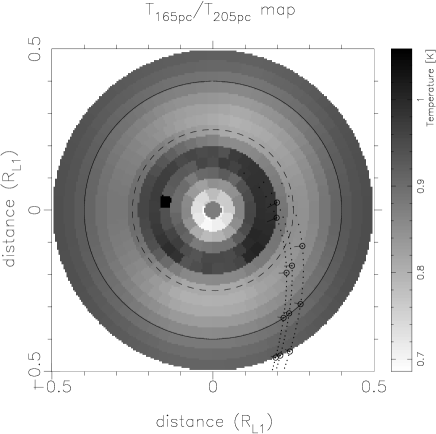
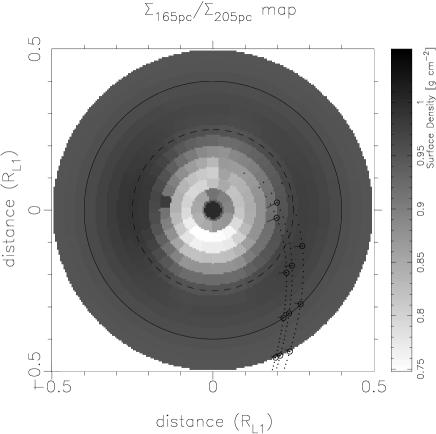
Figure 11: The ratio map in temperatures (left) and surface densities (right) for trial distances 165 pc (Wood et al. 1995) and 205 pc (PPEM, see Section 6). The Roche-lobe of the primary component lies just about outside the plotted region. The dashed line at 0.25$R_{\SS L1}$ and the solid line at 0.4$R_{\SS L1}$ are drawn for comparison with Fig. 5. The curved, dotted lines in the grey-scale plot are theoretical accretion stream paths for mass ratios 0.15 $\pm$ 50%. The secondary is at the bottom.

The artifical light curves were calculated using the same phase resolution as for the HT Cas data displayed in Fig. 1, i.e. 0.003 outside the eclipse (phases $\pm$0.065) and 0.0015 during eclipse yielding 112 data points between phases $\pm 0.1$. We added noise with a signal-to-noise level of 100. The correct distance was assumed to be 205 pc.

Fig. 10 shows the resulting entropy - distance relation. A parabolic fit to the data points peaks at 210 pc, i.e. at a distance 5 pc larger than the true distance.

In several applicaton we noticied that when fitting light curves, the distance decreases with decreasing $\chi^{2}$ (see e.g. Fig. 2). This effect is usually only small, about 5 pc for a drop in $\chi^{2}$ of 1. In applications to real data, one usually encounters a lower limit of $\chi^{2}$ below which no good fit to the data can be found (or the reconstructions start showing artefacts). This limit is determined by flickering in the data or by the adequacy of the spectral model used (for a discussion on the appropriateness of our model see Section resolution). We expect therefore, that the true distance will be slightly smaller than the derived distance.

Appendix B Reconstruction with smaller distance

To illustrate the difference between the maps for a trial distance of 165 pc as determined by Wood et al. (1995) and our PPEM distance estimate we plot the ratio of the parameter maps in Fig. 11. To allow comparison, we used the reconstructions for a $\chi^{2}$ of 2.5. An asymmetry can clearly be seen. Since the map for 205 pc is much smoother than the one for 165 pc, the asymmetry is mainly due to the latter map.

The temperature ratio map shows maxima in two areas at azimuths $\pm 90^{\circ}$, while the surface density ratio map shows a minimum at azimuth $0^{\circ}$. This shows that the algorithm tries to maintain the eclipse width and at the same time to reduce the emitting area, leading to a shortening of the disc along the binary axis and thus to an elongated emission structure perpendicular to the binary axis. Such an emission structure is usual for a reconstruction for which the trial distance is too small.

Additionally, the reconstruction shows a single hot pixel at approximately azimuth $-95^{\circ}$ and radius 0.15$R_{\SS L1}$. Such hot pixels are usually artefacts, since it is physically unlikely to maintain such a sharp gradient in temperature and in such a small area. It is especially unlikely since the light curves are averaged. Such a hot pixel is usually an additional indication for a false trial distance.

Appendix C Reconstruction with larger distance

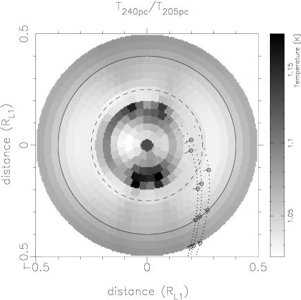
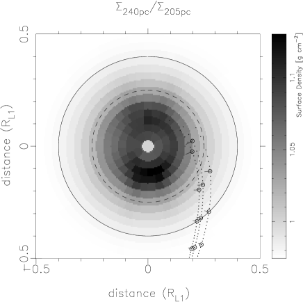
Figure 12: The ratio map in temperatures (left) and surface densities (right) for trial distances 240 pc (Wood et al. 1995) and 205 pc (PPEM, see Section 6). The Roche-lobe of the primary component lies just outside the plotted region. The dashed line at 0.25$R_{\SS L1}$ and the solid line at 0.4$R_{\SS L1}$ are drawn for comparison with Fig. 5. The curved, dotted lines in the grey-scale plot are theoretical accretion stream paths for mass ratios 0.15 $\pm$ 50%. The secondary is at the bottom.

For completeness we show the difference between the reconstructions for trial distances 240 and 205pc as a ratio of the parameter maps in Fig. 12. Again we used a $\chi^{2}$ of 2.5 for comparison. These maps show also an asymmetry, however, a distinctly different pattern. Since the map for 205pc is very smooth for a $\chi^{2}$ of 2.5, the asymmetry is mainly due to the map for 240pc.

The maps show maxima along an axis parallel to the binary axis. This can be understood if one considers the following: the eclipse width is defined by the eclipse profile and determines the extension of the accretion disc perpendicular to the binary axis. However, if the distance is too large, the disc needs to cover more area than available if the disc were axisymmetric. Therefore, the emission region in the disc extends along the binary axis without compromising the eclipse width. This pattern is thus typical for a map that was derived with too large a trial distance.

The reason for the enhanced structure in the disc is the same as for the curious hot pixel in the map reconstructed with the small distance.

Appendix D Reconstruction with partially visible white dwarf

Figure 13: The ratio of the temperature and surface density reconstructions using a partially visible white dwarf ($T_{wd/4}$, $\Sigma_{wd/4}$) and a fully visible white dwarf ($T_{wd/2}$, $\Sigma_{wd/2}$). The dashed line at 0.25$R_{\SS L1}$ and the solid line at 0.4$R_{\SS L1}$ are drawn for comparison with Fig. 4.

Since the inner part of the disc appears to be optically thick, the “lower” hemisphere of the white dwarf should be (at least partially) occulted. Therefore, we reconstructed the disc and white dwarf temperature with presetting the occultation of the central object.

These reconstructions show significantly more scatter than the ones shown in Fig. 4 for the fully visible white dwarf. This scatter is expressed by a much lower entropy of these maps compared to the ones using a fully viaible white dwarf: the value of the entropy is $-1.1\times 10^{-3}$, a factor of 3.5 below the one for the fully visible white dwarf and outside the plotted region in Fig. 2. Therefore, the PPEM reconstruction favors the fully visible white dwarf, like Horne & Wood (1990).

Fig. 13 shows the ratio of the two reconstructions. As expected, the white dwarf temperature in the case of the white dwarf with a smaller visible area is higher ($T_{wd,1/4}=26\,700$K). In addition to showing more scatter, the values of the disc temperatures and surface densities are generally higher. This is due to a combined attempt to reproduce sufficient total flux and the correct colours, since a slightly hotter white dwarf shows a slightly bluer spectrum.

Appendix E Reconstruction with various default maps

Figure 14: The entropy for reconstructions with various blurring parameters. The plot gives only the degree of blurring in azimuth, Tab. 2 also gives the amount of blurring in radius. The circles connected by the dashed lines are for solid arc smearing, the single point corresponds to solid angle smearing. The entropy for huge $360^{\circ}$ blurring is $-7.7\times 10^{-4}$ (it is omitted from the plot for clarity).

During the iteration of an eclipse mapping method like PPEM, the intermediate map is compared to a default map which in turn is adjusted at certain, predefined intervalls. The general use of a default map is explained in more detail in VHH99. In short: a default map is a smeered out version of an intermediate map calculated using certain blurring parameters in radial and azimuthal direction.

The default map therefore introduces a certain degree of symmetry or rather smoothness. The degree of smoothness depends on the value of the blurring parameter. It is important to note that at the usual blurring parameters (see below) asymmetries are not completely or even nearly completely suppressed. It only leads to a certain degree of smoothness in the disc. This is desireable in order to avoid artefacts to dominate the map and to choose one out of the many possible solutions.

In order to estimate the influence of the default map on the PPEM solution we used a set of default smearing parameters as given in Tab. 2. Usually, we use a solid arc smearing, i.e. we use a constant arc length. This leads to enhanced blurring in the central regions. We use this type of blurring, because we expect more large scale structures in the outer regions (e.g. non-circular disc, bright spot). In one case we used solid angle blurring, leading to enhanced blurring in the outer regions of the disc.

The reconstructed temperature ($T$) and surface density ($\Sigma$) maps all show similar absolut values for $T$ and $\Sigma$ only with a larger scatter in the maps corresponding to the larger blurring parameter values. As an indicator for the random scatter, Fig. 14 shows the entropy for the solutions using the blurring parameters as given in Tab. 2.

As surprizing as it seems to find a higher entropy for smaller blurring parameters, we have a simple explanation for this. Although the maps for smaller blurring parameters seem to have more scatter (Fig. 15), this is not random. The image in the map rather looks more focussed, tending to separate the pixels in the map into either hot or cool ones. Considering only the cool pixels, the disc is then very smooth. This way, artefacts are also enhanced and can easily be misinterpreted. We therefore prefer using intermediate blurring parameters and have used the ones called medium for our reconstructions.

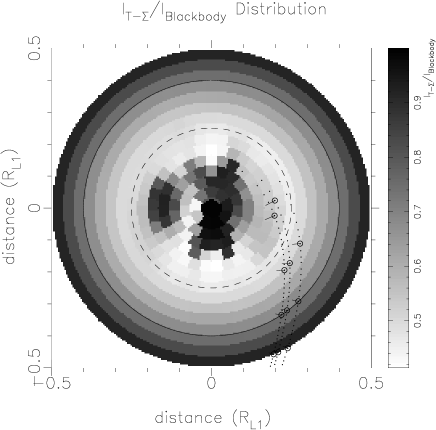
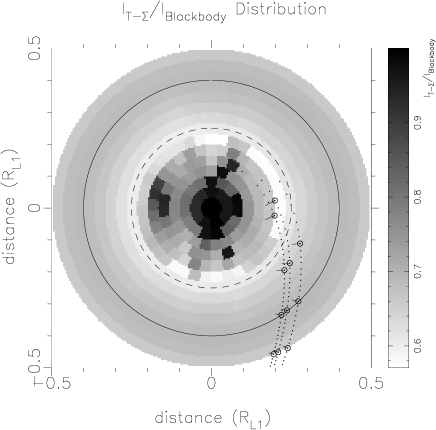
Figure 15: The intensity ratio maps for tiny and huge blurring parameters. The Roche-lobe of the primary component lies just about outside the plotted region. The dashed line at 0.25$R_{\SS L1}$ and the solid line at 0.4$R_{\SS L1}$ are drawn for comparison with Fig. 5. The curved, dotted lines in the grey-scale plot are theoretical accretion stream paths for mass ratios 0.15 $\pm$ 50%. The secondary is at the bottom.

Table 2: The blurring parameters. All but one default maps are calculated with solid arc blurring. For the only exception where we applied solid angle blurring, we used the medium blurring parameters.

description	Angle (∘)	Radius ($R_{\SS L1}$)
tiny	1	0.04
very little	2.5	0.1
little	5	0.2
medium	10	0.4
much	20	0.8
huge	360	0.4

Appendix F Reconstruction with cover factor $C<1$

Figure 16: The effective temperature reconstructed for a distance of 133 pc and a covering factor $C=0.41$. The underlying dotted lines are theoretical steady state temperature distributions for $\log\dot{\cal M}=13$ to 18, the one for $\dot{\cal M}=10^{16}$gs^-1 is drawn solid for reference. The dashed-dotted line indicates the critical mass accretion rates $\dot{M}_{\rm A}$ according to Ludwig et al. (1994). The dashed line at 0.25$R_{\SS L1}$ and the solid line at 0.4$R_{\SS L1}$ are drawn for comparison with Fig. 9.

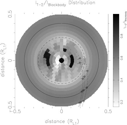
Figure 17: The intensity ratio maps for a distance of 133 pc and a covering factor $C=0.41$. The Roche-lobe of the primary component lies just about outside the plotted region. The dashed line at 0.25$R_{\SS L1}$ and the solid line at 0.4$R_{\SS L1}$ are drawn for comparison with the plot in Fig. 5 (right). The curved, dotted lines in the grey-scale plot are theoretical accretion stream paths for mass ratios 0.15 $\pm$ 50%. The secondary is at the bottom.

For completeness, we reconstructed the accretion disc for a distance of 133 pc implementing a covering factor $C=41\%$ for the disc emission. The resulting effective temperature ($T_{\mbox{\scriptsize eff}}$) map is shown in Fig. 16. The $T_{\mbox{\scriptsize eff}}$’s range mostly below or around the critical limit given by Ludwig et al. (1994), similar to the estimate for $d=133$ pc in Fig. 9. Fig. 17 reveals the structures in the disc. They are distinctly different to those in maps with distances $\neq 205$pc or constructed with small blurring parameters. We do not know whether these structures are real or new artefacts introduced into the maps. However, it is likely that the covering factor is not constant as assumed in this calculation and that a reconstruction with $C$ as a parameter map will result in more realistic solutions.

The white dwarf temperature is reconstructed to $T_{wd}=17450K$, compatible with Wood et al.’s (1995) estimate of $18\,700\pm 1\,800$ K, especially taking into account that they used a slightly larger distance.

References

- [1] Adam J., Stoerzer H., Wehrse R., Shaviv G., 1986, ApJ 305, 740
- [2] Barnes T.G., Evans D.S., Moffett T.J., 1978, MNRAS 183, 285
- [3] Berriman, G., Szkody, P., Capps, R. W., 1985, MNRAS, 217, 327
- [4] Berriman G., Kenyon S., Boyle C., 1987, AJ, 94, 1291
- [5] Beuermann K., Baraffe I., Kolb U., Weichhold M., 1998, A&A 339, 518
- [6] Beuermann K., Baraffe I., Hauschildt P., 1999, A&A 348, 524
- [7] Beuermann K, Weichhold M., 1999, Annapolis Workshop on Magnetic Cataclysmic Variables, ASP Conference Series, Vol. 157, eds. C. Hellier, K. Mukai, p. 283
- [8] Bruch, A. 1992, A&A, 266, 237
- [9] Frank J., King A., Raine D. 1992, “Accretion Power in Astrophysics”, Cambridge Astrophysics Series, Cambridge University Press, p. 81
- [10] Hoffmann B., Hessman F.V., Reinsch K., “Kepler Tomography of the Accretion Disk in V436 Centauri”, in Proc. of Conf. Physics of Cataclysmic Variables, ASP Conf. Ser., in press
- [11] Horne K., 1985, MNRAS 213, 129
- [12] Horne K., Marsh T.R., 1986, MNRAS 218, 761
- [13] Horne K., Saar S.H., 1991, ApJ, 374, L55
- [14] Horne K., Wood J.H., Stienning R.F., 1991, ApJ, 378, 271 (HWS91)
- [15] Hubeny I., 1991, in IAU Colloq. 129, Structure and Emission Properties of Accetion Disks, eds. C. Bertout, S. Collin, J.-P. Lasota, J. Tran Thanh Van (Singapure: Fong & Sons), p. 227
- [16] Kirkpatrick, J.D., McCarthy, D.W. 1994, AJ, 107, 333
- [17] Leach, R., Hessman F.V., King A.R., Stehle, R., Mattei, J. 1999, MNRAS 305, 225
- [18] Littlefair S.P., Dhillon V.S., Marsh T.R., Harlaftis E.T., 2001, MNRAS 327, 475
- [19] Ludwig K., Meyer-Hofmeister E., Ritter H., 1994, A&A 290, 473
- [20] Marsh T.R., 1990, ApJ, 357, 621
- [21] Marsh T.R., Horne K., 1990, ApJ, 349, 593
- [22] Marsh T.R., Horne K., Schlegel E.M., Honeycutt R.K., Kaitchuck R.H., 1990, ApJ, 364, 637
- [23] Meyer F., Meyer-Hofmeister E., 1994, A&A, 288, 175
- [24] Patterson J., 1981, ApJS 45, 517
- [25] Schreiber M.R., Gänsicke B.T., Cannizzo J.K., 2000, A&A 362, 268
- [26] Shakura N.I., Sunyaev R.A., 1973, A&A, 24, 337
- [27] Skilling J., Bryan R.K., 1984, MNRAS 211, 111
- [28] Smak J., 1989, AcA 39, 201
- [29] Smak J., 1982, AcA 32, 199
- [30] Smak J., 1984, PASP, 96, 5
- [31] Smak J., 1989, AcA 39, 201
- [32] Steeghs D., Harlaftis E.T., Horne K., 1997, MNRAS 290, L28
- [33] Vrielmann S., 2001, In: “Astro Tomography”, ed. H. Boffin, D. Steeghs, J. Cuypers, Lecture Notes in Physics 573, Springer-Verlag, p. 332
- [34] Vrielmann S., Horne K., Hessman F.V., 1999, MNRAS, 306, 766 (VHH99)
- [35] Vrielmann, S., Still, M., Horne, K. 2001, “Imaging accretion discs with Hubeny spectra” In: “The Physics of Cataclysmic Variables and Related Objects”, Göttingen, August 5-10 2001, ed. B. Gänsicke, K. Beuermann, K. Reinsch, ASP conference series, in press
- [36] Vrielmann S., Stiening R., Offutt W., 2002, MNRAS, submitted
- [37] Welsh, W.F., Wood, J.H., Horne, K. 1996, in “Cataclysmic Variables and related objects”, Keele, June 26-30, 1995, ed. A. Evans, J.H. Woods, Dordrecht: Kluwer Academic Publishers, p. 29
- [38] Wenzel W., 1987, AN, 308, 75
- [39] Wood J.H., Horne K., 1990, MNRAS, 242, 606
- [40] Wood J.H., Horne K., Vennes S., 1992, ApJ, 385, 294 (WHV92)
- [41] Wood J.H., Naylor T., Hassall B.J.M., Ramseyer T.F., 1995, MNRAS, 273, 772
- [42] Yonehara, Mineshige & Welsh 1997, ApJ, 486, 388
- [43] Young P., Schneider D.P., Shectman S.A., 1981, ApJ, 245, 1035