A Proper Motion Survey for White Dwarfs with the Wide Field Planetary Camera 2

Abstract

We have performed a search for halo white dwarfs as high proper motion objects in a second epoch Wide Field Planetary Camera 2 image of the Groth-Westphal strip. The survey covers 74.8 arcmin², and is complete to $V\sim 26.5$. We identify 24 high proper motion objects with $\mu>0.014^{\prime\prime}$/y. Five of these high proper motion objects are identified as strong white dwarf candidates on the basis of their position in a reduced proper motion diagram. We also identify two marginal candidates whose photometric errors place them within $\sim 1\sigma$ of the white dwarf region of the reduced proper motion diagram. We create a model of the Milky Way thin disk, thick disk and stellar halo and find that this sample of white dwarfs is clearly an excess above the $\leq 2$ detections expected from these known stellar populations. The origin of the excess signal is less clear. Possibly, the excess cannot be explained without invoking a fourth galactic component: a white dwarf dark halo. Previous work of this nature has separated white dwarf samples into various galactic components based on kinematics; distances, and thus velocities, are unavailable for a sample this faint. Therefore, we present a statistical separation of our sample into the four components and estimate the corresponding local white dwarf densities using only the directly observable variables, $V$, $(V-I)$, and $\vec{\mu}$. For all Galactic models explored, our five white dwarf sample separates into about 3 disk white dwarfs and 2 halo white dwarfs. However, the further subdivision into the thin and thick disk and the stellar and dark halo, and the subsequent calculation of the local densities are sensitive to the input parameters of our model for each Galactic component. Using the lowest mean mass model for the dark halo and the 5 white dwarf sample we find $n_{0,{\rm thin~{}disk}}=2.4^{+0.7}_{-0.6}\times 10^{-2}$ pc^-3, $n_{0,{\rm thick~{}disk}}=0.0^{+7.6}\times 10^{-4}$ pc^-3, $n_{0,{\rm stellar~{}halo}}=0.0^{+7.7}\times 10^{-5}$ pc^-3, and $n_{0,{\rm dark~{}halo}}=1.0^{+0.4}_{-0.4}\times 10^{-3}$ pc^-3. This implies a 7% white dwarf halo and six times the canonical value for the thin disk white dwarf density (at marginal statistical significance), but possible systematic errors due to uncertainty in the model parameters likely dominate these statistical error bars. The white dwarf halo can be reduced to $\sim 1.5$% of the halo dark matter by changing the initial mass function slightly. The local thin disk white dwarf density in our solution can be made consistent with the canonical value by assuming a larger thin disk scaleheight of 500 pc.

1 Introduction

The microlensing results towards the Large Magellanic Cloud (Alcock et al., 1997, 2000; Lasserre et. al., 2000) generated much interest in the possibility of white dwarfs (WD) as significant contributors to the Galactic halo dark matter. The most recent results suggest a most likely MACHO fraction of 20% and a most likely MACHO mass between 0.15 and 0.9 $M_{\odot}$ (Alcock et al., 2000). Other MACHO candidates such as brown dwarfs, M dwarfs, and neutron stars are excluded, respectively, on the basis of the most likely MACHO mass, direct star counts which suggest that their contribution to the total mass is insignificant (Gould, Flynn & Bahcall, 1998) and entirely unacceptable nucleosynthesis yields from their main sequence precursors (Carr, 1994).

White dwarfs are well-known low luminosity stars, and have been extensively surveyed, for instance by Legget, Ruiz & Bergeron (1998) and Knox, Hawkins & Hambly (1999). A very recent report Majewski & Siegel (2001) suggests the scale height for thin disk white dwarfs may be higher than previously thought, and that consequently the total number of thin disk white dwarfs is also higher than previously thought.

White dwarfs as dark matter pose their own set of problems, as their main sequence progenitor may produce more metals (He, C, N) than observed (Fields, Freese & Graff, 2000). These chemical evolution constraints can possibly be avoided by assuming a non-standard initial mass function (Chabrier, Segretain & Méra, 1996; Chabrier, 1999) and, perhaps, lower metal yields from Z=0.0 zero age main sequence progenitors. Recent results (Marigo et al., 2001) suggest that the first-dredge up does not take place for zero metallicity stars with $M\gtrsim 1.2~{}M_{\odot}$. Further, the second dredge-up is suppressed for zero metallicity stars with $M\lesssim 2.1~{}M_{\odot}$ and only brings CNO to the surface for $2.7~{}M_{\odot}\lesssim M\lesssim 8.3~{}M_{\odot}$. Finally, thermal pulses on the asymptotic giant branch which would normally bring carbon to the surface may not occur (Chabrier, 1999; Marigo et al., 2001).

Interest in WD as directly detectable dark matter intensified with the suggestion that ancient hydrogen atmosphere WD evolve towards bluer optical colors as they cool (Hansen, 1998), remaining detectable in the $V$ band for many Gyr longer than previously assumed. This provided a plausible explanation for some of the faint blue objects in the Hubble Deep Field (HDF), two of which were reported to have proper motions consistent with an interpretation as ancient halo white dwarfs (Ibata et al., 1999).

Although the HDF moving objects were determined to be false detections (Richer, 2001), excitement over the possibility of halo white dwarfs was renewed with the results of Oppenheimer et al. (2001) who claim detection of 38 halo white dwarfs, constituting at least 2% of the Galactic halo dark matter. Oppenheimer et al. (2001) present their results in the form of a plot of the galactic radial (U) and rotational (V) velocities of each WD and superimpose 1 and 2 sigma contours for the expected locations of the thick disk and halo components of the Milky Way. White dwarfs lying outside the 2 sigma contours of the thick disk are assumed to belong to a halo population.

Reid, Sahu & Hawley (2001) provide an alternate interpretation of the Oppenheimer et al. (2001) results, arguing the velocity distribution is more consistent with the high-velocity tail of the thick disk. Furthermore, by comparing the placement of the halo candidates along a fiducial WD evolution track in a color-magnitude diagram, Hansen (2001) notes that the Oppenheimer et al. (2001) halo population seems to have an age distribution similar to the standard thin disk population. Hansen (2001) finds that it is difficult to make the age distribution of this sample consistent with common assumptions about thick disk star formation (a simple burst at early times), and even more difficult to achieve consistency with some sort of truly ancient halo population. Koopmans & Blandford (2001) extend this argument, noting that the thick disk and halo WD populations (as divided by Oppenheimer et al. (2001)) are indistinguishable in terms of luminosity, color and apparent age.

Koopmans & Blandford (2001) undertake a more sophisticated analysis of the Oppenheimer et al. (2001) sample, calculating the contribution of the thick disk and halo using a maximum likelihood analysis. They find a local number density of thick disk WD of $n_{0,{\rm thick~{}disk}}=1.8\pm 0.5\times 10^{-3}$ pc^-3 and a local number density of halo WD of $n_{0,{\rm halo}}=1.1^{+2.1}_{-0.7}\times 10^{-4}$ pc^-3. The halo density is about 5 times higher then previously expected (Gould, Flynn & Bahcall, 1998), but constitutes only $\sim$ 0.8% of the dark halo density, at least an order of magnitude smaller than the MACHO density implied by the microlensing results.

Reyle, Robin & Creze (2001) also provide a reanalysis of the Oppenheimer et al. (2001) sample. These authors use a comprehensive description of Galactic stellar populations to provide a simulation of the Oppenheimer et al. (2001) data, including the detection limits in proper motion, magnitude and color. They conclude that thick disk white dwarfs with standard local densities are sufficient to explain the Oppenheimer et al. (2001) sample.

The wide spread in age of the Oppenheimer et al. (2001) sample has led several parties to suggest that these WD originated in the thin disk, but were subsequently accelerated to much higher velocities. Koopmans & Blandford (2001) suggest a mechanism to eject WD into the halo with the required speeds of $\sim 200$ km/s through the orbital instability of triple systems. Davies (2001) proposes another binary driven mechanism in which the secondary of a tight binary system (the WD progenitor) is ejected at high velocity when the primary explodes as a supernova.

The Oppenheimer et al. (2001) results are based on a very wide survey (10% of the sky) with a bright limiting magnitude ($R_{\rm lim}\lesssim 20$). In this work we take the opposite approach, examining a very small area of the sky (20 Wide Field Planetary Camera 2 fields), but probing to a very deep limiting magnitude ($V_{\rm lim}\sim 27$). Based on the Oppenheimer et al. (2001) results which are $\sim 90$% proper motion limited (Koopmans & Blandford, 2001), we would not expect the white dwarf luminosity function to rise suddenly beyond their detection limit. However, the Oppenheimer et al. (2001) survey cannot exclude the existence of an ancient “dark halo” white dwarf population of age $>>10$ Gyr.

In fact, since Oppenheimer et al. (2001) use the Bergeron, Ruiz & Leggett (1997) survey of young white dwarfs to derive a linear relationship between absolute magnitude and color, they assume that all detected white dwarfs are younger than the beginning of the cooling turnoff towards bluer colors in the color magnitude diagram. In their filters, this color turnoff occurs at a temperature of around 2500 K, or a white dwarf age of about 13-14 Gyr. Since they observe very few white dwarfs near the color turnoff this is probably a good, if limiting, assumption.

Although we initially explore an intuitive analysis of our sample along the same lines as Oppenheimer et al. (2001), in our final analysis we avoid making any assumptions about the age of our sample and estimate the local densities of disk and halo white dwarfs based solely on the observed properties of our sample: apparent magnitude, color and proper motion vector on the sky.

This work is structured as follows. In §2 we describe the observation and reduction of each epoch, our procedure for matching stars between epochs, the selection of significant high proper motion objects and the results of our completeness tests. In §3 we describe our selection criteria for white dwarfs and examine their kinematic properties in a manner similar to Oppenheimer et al. (2001). In §4 we model various components of the Milky Way and compute the number of white dwarf detections we expect in our survey. Then, using only the directly observable properties, we create a method to statistically separate our sample into the various Milky Way components. We conclude in §5.

2 Groth Strip Observations and Reductions

First epoch images of the “Groth-Westphal strip” (Groth et al., 1994) were taken by the Wide Field Planetary Camera 2 (WFPC2) in the F606W and F814W filters between March 7, 1994 and April 8, 1994. This dataset consists of 27 adjacent WFPC2 fields taken at high galactic latitude ($l\sim 96^{\circ}$, $b\sim 61^{\circ}$). Each first-epoch field covers 4.4 arcmin², consists of 4 raw exposures per filter and has a combined exposure time of 4400s in the standard Hubble Space Telescope (HST) I-band (F814W) and 2800s in a narrow band V (F606W).

A re-imaging of 17 fields of the Groth strip, comprising 74.8 arcmin², was taken by the WFPC2 in a single filter (F606W) in March, 2001, giving us a baseline of 7 years between epochs. Each second-epoch field consists of 6 raw exposures and has a combined exposure time of 4200s.

2.1 Photometry

Because the Groth strip lies at such high galactic latitude, the fields are nearly devoid of bright stellar objects, containing $\sim 4$ stars of $V<26$ per WFPC2 chip. This makes it difficult to compute exact transformations between the multiple raw images of the same field, especially as the raw images are heavily contaminated by incident cosmic ray particles. Thus, in combining the raw images we assume that the requested pointing offsets between raw images (commonly called dithers) were accurate and the images were combined using these offsets. Generally, WFPC2 pointings are accurate to $\sim 0.1$ WF pixels, so this assumption does not add serious error to the procedure. The first epoch images are all taken at the same pointing (un-dithered) so the raw images are combined with zero offset. The second epoch images are dithered by non-integer values. We list the fields and times observed in Table 1.

After the raw images were aligned, all subsequent processing and reductions were performed using the HSTphot package made publicly available by Andrew Dolphin (Dolphin, 2000). Each raw image is first masked using the bad pixel mask. The aligned raw images are then combined and cleaned of cosmic rays. For each pixel, the cosmic ray cleaning algorithm computes the median pixel value, a photon counting uncertainty ($\sigma$) based on the median value, the exposure time, read noise and gain. The uncertainty is then given an additional contribution added in quadrature to account for the registration uncertainty. Pixel values which were more then $3\sigma$ from the median value were rejected and the remaining pixel values were averaged.

Point-spread fitting (PSF) photometry was performed on the combined images using the HSTphot package. The HSTphot package includes a library of PSFs constructed with the Tiny Tim software. For the F814W filter it also includes default residuals to the “perfect” Tiny Tim PSFs. In addition, HSTphot also allows the PSF to be adjusted based on measurements made on suitable stars in the user’s program frames. In the Groth strip frames, there are very few stars with enough counts to act as suitable PSF stars. Attempts to adjust the PSF using available stars resulted in unusual looking PSFs, although the final results were insensitive to the PSF used (see below). Thus, in the final reductions we forced HSTphot not to adjust its PSF based on our program frames. For the F814W band reductions we allowed it to use the default residuals. According to the HSTphot documentation, not adjusting the PSF based on the program stars can create a systematic error of up to $\pm$0.1 magnitudes for faint stars. We allowed HSTphot to internally compute aperture corrections. The HSTphot magnitudes were converted to Landolt $V$ and $I$ using the synthetic transformations of Table 10 from Holtzman et al. (1995b).

HSTphot also includes an object classification routine which divides objects into stars, possible unresolved binaries, single-pixel cosmic rays or extended objects. HSTphot was designed for crowded stellar fields and the use of this software on fields of mostly galaxies is certainly an application beyond its intended purpose. Thus, it is unsurprising that the object classification routine was often unreliable, classifying objects as stellar which, upon inspection seemed more likely to be galactic. Regardless of the output classification, HSTphot fits a stellar PSF to all objects and the output magnitude and centroids are based on this fit. The quality of its output is thus directly related to whether or not the object was actually a point source.

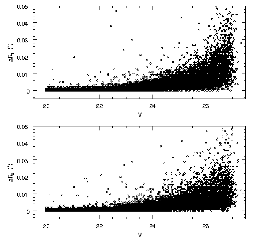
Figure 1: The uncertainty in the centroids computed by HSTphot as a function of $V$ magnitude. The uncertainty is estimated using our artificial star tests. $\Delta R_{1}$ indicates the difference between the input and recovered centroid for artifical stars in the epoch 1 frames. $\Delta R_{2}$ indicates the same quantity for epoch 2.

We estimate a total photometric error for faint objects ($V\lesssim 24$) of $\sim 0.15$ mag with contributions from both the non ideal PSF and photon counting error. We can use the artificial star tests (described in § 2.4) to estimate the centroid accuracy of HSTphot for stellar objects by computing the difference between the input and recovered centroid. The centroid uncertainty as a function of magnitude for all artifical stars is shown in Figure 1. This uncertainty is underestimated in the sense that it tests the ability of HSTphot to centroid objects with a perfect PSF. The artificial star tests add stars to frames with the same PSF (plus random noise) with which they are recovered. Since this PSF is not perfect for the real stars in our frame, the centroid uncertainty for real stars is likely substantially higher. The greater uncertainty in the centroids for real stars is reflected in final uncertainty in the coordinate transformation between epochs (see § 2.2) which is much larger than the HSTphot centroid uncertainty of Figure 1.

2.2 Matching stars between epochs

Accurate computation of the transformation between two epochs of a field is best performed using many, bright, point-like sources. Bright stellar sources are in short supply in the Groth strip and we are forced to compromise to some extent.

The first step in computing transformations between two WFPC2 frames is to correct for the geometric distortion of the chips. There are several sets of distortion coefficients available including one specifically optimized for the first epoch Groth strip (Ratnatunga, Ostrander & Griffiths, 1997), but the most widely employed are from Holtzman et al. (1995a). Each set of coefficients can also put the four WFPC2 chips on a single “global” coordinate frame. Since the accuracy of our transformations is limited by the low number of sources per field, a global coordinate system would seem to be a useful tool. We experimented with transformations based on several different global coordinate systems and always found the residuals of these transformations to depend heavily on the X or Y position of the star on the chip. This problem arises not from the distortion coefficients themselves but from the fact that the geometric transformation of WFPC2 has a small time dependence, primarily in the interchip separation which can vary by as much as 150 mas. Thus, there exists no global distortion solutions that work well on both the first epoch (1994) and second epoch (2001) data. This limited us to computing local transformations on a chip by chip basis using the Holtzman et al. (1995a) distortion coefficients.

Since the reduction of this data (in April 2001) a new set of distortion coefficents has become available (WFPC2 Instrument Science Report 2001-10). We have tested a reduction routine in which we use the Holtzman et al. (1995a) distortion coefficients for our epoch 1 data and the new distortion coefficients for our epoch 2 data. We find no significant improvement in our results. The dominant source of uncertainty in our transformations arises from our imperfect PSF and the small number of objects in our fields, not the distortion correction used.

Because we were unable to use global transformations, we were also unable to use the data in the Planetary Camera (PC). The extremely small area of the PC ($\sim 0.3$ square arcminutes) rarely encompassed enough objects in the frame with which to compute local transformations. For consistency, we simply ignore all PC data.

Before performing the transformations, we developed an object classification routine based on the SExtractor software (Bertin & Arnouts, 1996). SExtractor identifies objects above a certain threshold and then utilizes a neural network classification routine to assign each object a decimal number between 0 and 1 where 0 indicates a stellar (point-source) object and 1 indicates a galactic (extended-source) object. Initially, we computed transformations based only on objects that were classified as stellar by SExtractor with the appropriate centroids taken from the HSTphot output. For many chips there simply were not enough such stellar objects to compute transformations. Thus, we developed a routine where transformations were computed using stellar objects and “small, round” galaxies. After much experimentation we found that better transformations were obtained from HSTphot centroids (PSF fitting centroids) for both stars and galaxies than from using the SExtractor centroids for the galaxies. Computing the coordinate transformations is an iterative procedure, in which we remove objects with residuals greater then 3 sigma before computing the final transformations. Final transformations computed are a full 6 parameter fit allowing for translation, rotation and change of scale. Our transformations are computed assuming that the vector sum of the proper motions over all stars and galaxies was zero.

In Figures 2 and 3, we plot the residuals to the coordinate transformation between epochs for all Groth fields, $\Delta X$ and $\Delta Y$ as a function of X and Y position on the chip, magnitude, and radius from the distortion center at $(X,Y)=(354,344)$. The residuals show no obvious dependence on position indicating that we have corrected for the geometric distortion of the chips. The residuals show some dependence on magnitude, increasing towards fainter magnitudes. We compute the transformations and residuals only for stars with $V<26$ although we allow fainter stars to appear in the final list of matched stars for a frame. The main reason for this is that below $V\sim 26.5$ real stars in epoch 2 start to get matched with noise in epoch 1 (epoch 2 is $\sim 0.5$ magnitude deeper). Since the final high proper motion star lists are inspected by hand (see below), it is acceptable to include ill-matched stars in the final matched lists, but it is crucial that we minimize their occurrence in the list of stars used to compute the transformations.

The transformation residuals are used to compute standard deviations in x and y, $\sigma_{x}$ and $\sigma_{y}$, and then we define the total standard deviation as $\sigma=\sqrt{\sigma_{x}^{2}+\sigma_{y}^{2}}$. In Figure 4 we show a vector plot of the residuals for all stars used to compute the transformations in all fields as a function of position on the WFPC2 chip. The sigma for all fields combined is $\sigma=0.031^{\prime\prime}$.

Our final uncertainty in the coordinate transformation, $\sigma=0.031^{\prime\prime}$ is a substantially worse result then the limits reached by Anderson & King (2000). Our analysis is limited in comparison to their work in several respects. First, we cannot derive an effective PSF as we have virtually no suitable PSF stars and the first epoch was undithered. Without dithering and a large sample of PSF stars one cannot hope to adequately sample the pixel phase space and derive an effective PSF. Second, we have very few point sources per frame (a median value of 4 per chip) with which to derive transformations. Although we supplement the point source centroids with centroids of small galaxies, our ability to derive accurate transformations suffers as a result of the non point source PSF of the galaxies. We note that our estimate of 4 stars per chip is in line with the previous first epoch Groth strip reductions of Gould, Bahcall & Flynn (1997) who find an average of 3.1 M dwarfs per chip.

2.3 High Proper Motion Objects

Once the transformations were computed, lists of matching objects with $V\leq 27$ were made. Objects were matched to their nearest neighbor to a maximum of $0.75^{\prime\prime}$ and were considered matched only if the $V$ magnitude in each epoch matched to within 0.5 mag. An object was considered to have a significant movement between epochs and is hereafter known as a high proper motion object if the residual to the transformation for that object was above the maximum value of 3$\sigma$ for that field or $0.1^{\prime\prime}$ (1 pixel). That is, the proper motion limit is defined as

$$\mu_{\rm lim}\cdot\Delta t={\rm min}(3\sigma,0.1^{\prime\prime})$$ (1)

In order to minimize confusion while matching stars between epochs, we chose an upper proper motion limit of 7.5 pixels, or $\mu_{max}\sim 0.1^{\prime\prime}$/yr. Each high proper motion object was inspected by hand to verify that it was a plausible match between epochs and possessed a stellar PSF.

In Figure 5, we plot the vector proper motion as a function of the location on the WFPC2 chip for all high proper motion (HPM) objects. Averaged over all chips and all fields, the expected distribution of high proper motion objects over the face of the chip should be roughly uniform. We do not see any obvious departures from non-uniformity. Most importantly, we do not see any clustering of barely significant HPM objects towards the edges of the chip where the geometric distortions are most severe.

We repeated the full analysis using the adjustable PSF option in HSTphot. While a few barely significant movers in the constant PSF reduction were not significant in the adjustable PSF option and vice versa, the list of HPM objects was similar. All final WD candidates discussed below appeared in both the adjustable and constant PSF reductions.

2.4 Completeness tests

We performed completeness tests by adding artificial stars to the $V$ band images from both epochs. We compute the completeness fraction as a function of both magnitude and proper motion. First, coordinates for the star in epoch 2 were chosen randomly. We then compute the corresponding position in the epoch 1 frame using the derived transformations and apply a random offset (proper motion) of $-3\leq\Delta x\leq 3$, $-3\leq\Delta y\leq 3$ pixels before adding the star to the epoch 1 frame. If the transformed position does not lie on the epoch 1 frame, the star is not added to either epoch frame. Because of this, the effective area of our survey is only the area in which we have complete overlap between the two epochs. We create 25 frames each containing 20 artificial stars in each camera.

The artificial frames are then run through the standard photometric analysis. We do not recompute the transformations between epochs for the artificial frames. In this sense, the proper motion axis of the completeness test is artificial - since we add stars with the correct transformation, of course we recover them with the same transformation. Our completeness fraction is thus uniform in proper motion and really depends only on the $V$ magnitude. The completeness fraction as a function of $V$ magnitude and proper motion is shown in Figure 6. Since we compute our completeness fraction only in $V$ (and not $I$) the calibrated magnitudes of the artificial stars are computed without a color term.

We compute our completeness as a function of $\mu$ only to 4.25 pixels, yet in our analysis we accept objects in our samples with proper motions of up to 7.5 pixels. We chose the 4.25 pixels to be large enough to include the range of all observed high proper motion objects, yet small enough to allow good coverage in $\mu$ in a reasonable amount of computation time. As discussed above, our efficiencies do not depend on $\mu$ and we expect no dependence to arise if our efficiency calculation were extended to 7.5 pixels.

We expect that the detection efficiency should fall to exactly zero at $V=27.0$ as we do not allow stars with $V<27.0$ to appear in the final list of matched stars. The detection efficiency is not quite zero in this plot because we calculate the efficiency as a function of $V_{input}$ and we recover a very small fraction of stars that have $V_{input}>27.0$ but are recovered at $V<27.0$ and thus appear in the final matched lists.

Our completeness fraction falls rapidly to zero at $V\sim 26.5$, suggesting a limiting magnitude $V_{\rm lim}\sim 26.5$.

3 White dwarf candidates

3.1 Selection criteria and reduced proper motions

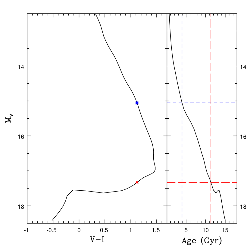
Figure 7: Cooling curves for a 0.6 $M_{\odot}$ WD from the models of (Richer et al., 2000). As WD cool $H_{2}$ molecules form in the atmosphere and create an opacity which is very strong in the near infra-red and forces the flux to emerge at bluer wavelengths. Thus, in a $V$ versus $(V-I)$ color magnitude diagram a WD initially cools along a blackbody curve, but eventually the WD start to become blue again. Because of this bend in the cooling track, a given $(V-I)$ color intersects the cooling curve at two points (black dotted line) , giving both a “young” (blue square and short-dashed lines) and an “old” solution (red triangle and long-dashed lines.

After an initial period of nearly blackbody cooling towards longer wavelengths, ancient white dwarfs experience a color turnoff and start to cool towards bluer wavelengths (Hansen, 1999). An example cooling curve of a 0.6 $M_{\odot}$ WD is shown in Figure 7. Thus, we expect to detect halo white dwarfs as blue objects with high proper motions. One way to isolate such candidates is on the basis of a reduced proper motion versus color diagram.

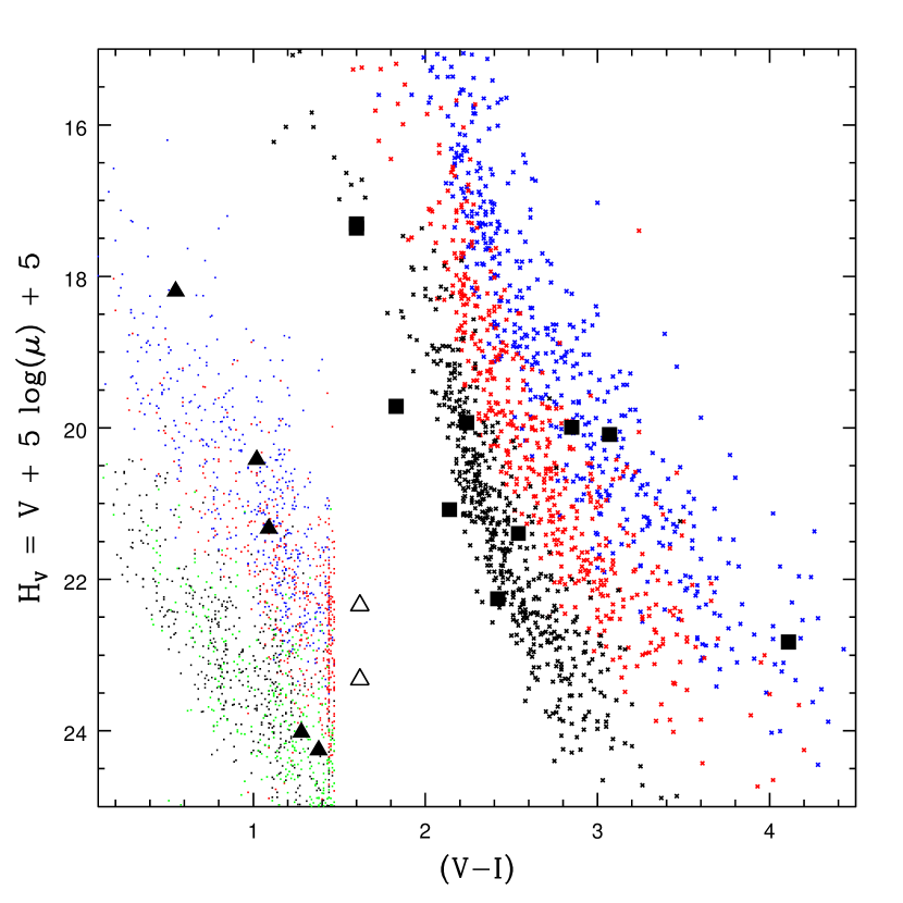
Figure 8: Reduced proper motion diagram for all HPM objects in the Groth Strip. The strong WD candidates are shown as filled black triangles, the nearby HPM main sequence stars are shown as filled black squares. The open triangles indicate the two marginal white dwarf candidates discussed in §3.1. The small dots indicate a simulated sample of detectable WD in the thin disk (blue), thick disk (red), stellar halo (black) and dark halo (green). The small crosses indicated a simulated sample of low mass main sequence stars ($M<0.9M_{\odot}$) from the thin disk (blue), thick disk (red) and stellar halo (black).

In Figure 8 we show the reduced proper motion diagram for all the significantly moving (high proper motion) objects in the Groth strip. The reduced proper motion is defined as $H_{V}=V+5\log(\frac{\mu}{{}^{\prime\prime}/{\rm yr}})+5=M_{V}+5\log(\frac{v_{t}}{\rm{km/s}})-3.378$. For an ensemble of objects with similar transverse velocities, $v_{t}$, an $H_{V}$ versus color diagram is an estimate of the color-absolute magnitude diagram where the magnitude axis has been shifted by some arbitrary constant. In Figure (8) we show the Groth strip HPM objects as large triangles and squares.

On the left hand side of Figure 8 we show a random sample of detectable white dwarfs from the thin disk (blue dots), thick disk (red dots), stellar halo (green dots) and dark halo (black dots). The parameters determining the geometry and stellar content of each Galactic components and our method for determining detectability will be discussed further in § 4. We note that the five HPM objects marked as filled black triangles fall over plausibly dense regions of the simulated white dwarf dots.

On the right hand side of Figure 8 we show a random sample of detectable low mass main sequence stars $(M<0.9M_{\odot})$ from the thin disk (blue crosses), thick disk (red crosses) and stellar halo (black crosses). The parameters of the Galactic components are the same as for the WDs and we use the low mass main sequence tracks from Baraffe et al. (1998). The HPM objects shown as filled black squares fall on plausibly dense regions of the simulated low mass main sequence star crosses. If we had included higher mass main sequence stars, the density of points would fall off much slower at small $H_{V}$.

On the basis of this reduced proper motion diagram we identify the filled black triangles as strong white dwarf candidates and the filled black triangles as main sequence stars. The $V$ magnitude, $(V-I)$ color and proper motion, $\mu$, of the white dwarf candidates are shown in Table 2.

The two stars shown as open triangles have $V>26$ and $\mu=1.1\mu_{\rm lim}$ and $\mu=1.3\mu_{\rm lim}$, respectively, and fall in an unpopulated region of the reduced proper motion diagram. Since we calculate the 3$\sigma$ significant proper motion limit $\mu_{\rm lim}$ with stars of $V<26$ and the proper motions of these faint stars are only barely above the proper motion limit, it may be the case that these two stars are not HPM objects at all, but simply spurious detections at very faint magnitude. However, it may also be the case that these two stars are moving objects, and are in fact white dwarfs near the color-turnoff. To move these two objects into the white dwarf region of the reduced proper motion diagram would require an error of $0.15$ magnitudes in $(V-I)$ in either our photometry or the theoretical white dwarf cooling tracks. Since an error of this magnitude is plausible, we will later consider the possibility that these two objects may belong to our white dwarf sample. We include these two objects in Table 2 as marginal candidates.

As noted by Majewski & Siegel (2001), quasars (QSOs) can be an important contaminant of the white dwarf region of the reduced proper motion diagram. Majewski & Siegel (2001) investigate this issue in detail and conclude that the soundest way to to eliminate QSOs from a white dwarf sample is to choose only objects which move with some certain minimum proper motion. They suggest that QSOs are almost certainly detected at proper motion of less than four times the uncertainty (eg. $\mu<4\sigma$) and that objects with proper motions above this limit are more certainly WD. The condition $\mu>4\sigma$ is satisfied for all of our candidates (see Table 2).

Hereafter we shall refer to WD candidates 1-5 from Table 2 as our 5 WD sample. Since we have the most confidence in this sample we will devote most discussion to it. We will also discuss the possibility that the marginal candidates do belong to our WD sample and will refer to WD candidates 1-7 from Table 2 as our 7 WD sample. For the sake of completeness, we will also discuss the possibility that all of our faint candidates are in error and that only WD 1, 3 and 4 from Table 2 belong to our WD sample. This will be referred to as the 3 WD sample.

We emphasize that these are not spectrally confirmed WD. With the exception of the bright candidate at $V=20.7$ these objects are too faint to allow for spectral confirmation with present technology. We also note that the proper motion of these candidates has not been confirmed with a third epoch. A previous WFPC2 detection of high proper motion WD by Ibata et al. (1999) has recently been withdrawn after a third epoch revealed the reported proper motion to be a spurious measurement (Richer, 2001). We note that all our candidates have substantially higher counts in both epochs than the second epoch image of Ibata et al. (1999).

3.2 Kinematics

In order to determine the transverse velocity of each candidate, we must first determine its distance, or, equivalently, its absolute magnitude. In principle, this may be done by finding the intersection of the color of each candidate with an absolute magnitude versus color track, such as that shown in Figure 7. However, because of the color turnoff, the $(V-I)$ color does not uniquely determine $M_{V}$. Instead, for each candidate we have a “young” and an “old” solution as illustrated in Figure 7. For each solution we may calculate the distance, $d=10^{\frac{V-M_{V}+5}{5}}$ and the transverse velocity, $v_{t}=\mu d$, where $\mu$ is the proper motion. Both the young and old solutions for the WD cooling time, distance, and transverse velocity are shown in Table 2. We include error bars on the derived quantities (cooling time, distance, transverse velocity and absolute magnitude) by calculating the maximum and minimum values obtained while I adjusting the $V$ magnitude and $(V-I)$ color by one unit of error (0.15 mag for $V$ and 0.20 mag for $(V-I)$). We note that the cooling time is not the total age of the WD as it does not include the main sequence lifetime of the WD precursors.

In a simplistic sense, the marginal candidates have no solution for the derived parameters since they do not intersect a white dwarf track in $(V-I)$ color. We assume that it is plausible that the observed $(V-I)$ color is wrong by some small amount and that they may just barely intersect the reddest point of the theoretical white dwarf track. Since we assume they only barely intersect the tip of the color turnoff, they cross the white dwarf track at only one point and have only one solution.

Also, we note that even if all the “old” solutions are correct, most of our WD are located at least one thin disk scaleheight (300 pc) above the plane. We also include the proper motion in the direction of increasing Galactic longitude, $\dot{l}$, and latitude, $\dot{b}$ in Table 2. The spherical coordinate system employed implies that $\mu=\sqrt{(\dot{l}\cos{b})^{2}+(\dot{b})^{2}}$.

This two solution ambiguity is not present in brighter, ground based samples where the distance can be determined with a photometric distance relation. Such a relation is essentially a linear fit to the young branch of a WD track in a color-absolute magnitude diagram. One such relation is derived in Oppenheimer et al. (2001) using the Bergeron, Ruiz & Leggett (1997) sample of nearby white dwarfs for which parallax distances are available. The Oppenheimer et al. (2001) sample employs this relation without much fear of ambiguity because in their filters ($B_{J}$, $R59F$) the color turnoff does not occur until a cooling time of $\sim$13.5 Gyr. In contrast, in our filters, the color turnoff occurs at the relatively short cooling time of $\sim$10 Gyr.

In Oppenheimer et al. (2001), the white dwarfs are roughly divided into thick disk and halo components by examining the location of the white dwarfs on a $(U,V)$ diagram, the velocity components towards the Galactic center and in the direction of Galactic rotation, respectively. The authors are able to calculate space velocities without information about the radial velocites by assuming that the velocity out of the plane, $W$, is zero (the mean value for all stars in the disk). Since the Oppenheimer et al. (2001) sample is near the South Galactic cap, this is not a bad assumption in the mean.

We encounter several difficulties in determining the space velocities of our sample: the two solution distance ambiguity, the lack of radial velocities and a lower Galactic latitude ($b\sim 60^{\circ}$) at which it is more difficult to make assumptions about the contribution of the radial velocity to the space velocities. In the next section we attempt a division of our sample into various Galactic components without making assumptions about the distances and velocties of our WD candidates.

4 Simulations

In this section, we interpret our results in a method independent of the white dwarf distance and assumptions about the young or old solutions. Instead, we examine our sample using only the directly observable variables $(V,V-I,\vec{\mu)}$. We begin in §4.1 by determining the number of white dwarf detections we expect from known stellar populations and compare this to our observed number. In §4.2 we consider a possible contribution from a white dwarf dark halo. §4.1 and §4.2 define our reference model of the Galaxy. In §4.3 we attempt a statistical division of our sample into several galactic components. In §4.4 we discuss alternative models of the Galaxy. In §4.6 we discuss the possiblity of alternative WD samples.

4.1 Expected number of white dwarfs from known stellar populations

First, we construct a simulation of the local WD populations of the MW, calculate the expected number of WD detections from each population, and compare this number with the Groth strip observations. In principle, given a model for each Milky Way component, we are able to predict the number of expected WD detections because we have an accurate estimate of our detection efficiency as a function of both proper motion and magnitude.

In the simulation, we explore three known stellar components of the Milky Way: the thin disk, thick disk and stellar halo. Estimating the number of WD we can detect from each component requires the knowledge of many model parameters. These parameters include $n_{0}$, the local number density of WD, $\rho(R,z)$ or $\rho(r)$, the shape of the density function (in cylindrical $(R,z)$ or spherical $(r)$ coordinates), $v_{a}$, the asymmetric drift of the population, and ($\sigma_{U}$,$\sigma_{V}$,$\sigma_{W}$), the velocity dispersions towards the Galactic center, in the direction of Galactic rotation and out of the plane towards the Galactic North Pole. We also need a WD luminosity function suitable for the age distribution and initial mass function (IMF) of each component. For all components, we assume that the number density of WD has the same shape as the mass density, i.e. $n(R,z)=\rho(R,z)/\bar{m}_{WD}$ where $\bar{m}_{WD}$ is the mean WD mass.

We model the Milky Way thin and thick disks as double exponentials of form

$$n_{\rm disk}(R,z)=n_{c}~{}\exp\left(-\frac{R}{R_{d}}-\left|\frac{z}{z_{d}}\right|\right)~{},$$ (2)

where $R$ and $z$ are cylindrical coordinates with origin at the Galactic center, $R_{d}$ is the scale length, $z_{d}$ is the scale height and $n_{c}$ is the central density. The central density is determined from the local density by $n_{c}=n_{0,{\rm disk}}\exp{(R_{0}/R_{d})}$ and $R_{0}=8.5$ kpc is the radius of the solar circle.

For the thin disk, we use the parameters $R_{d}=4$ kpc and $z_{d}=0.3$ kpc. (Note that Majewski & Siegel (2001) argue for a larger scale height for the thin disk.) The thin disk velocity dispersions and asymmetric drift are taken to be $(\sigma_{U},\sigma_{V},\sigma_{W})=(34,21,18)$ km/s and $v_{a}=6$ km/s (Binney & Tremaine, 1998). For the thick disk we use the parameters $R_{d}=4$ kpc and $z_{d}=1.0$ kpc. The thick disk velocity dispersions and asymmetric drift are taken to be $(\sigma_{U},\sigma_{V},\sigma_{W})=(61,58,39)$ km/s and $v_{a}=36$ km/s (Binney & Tremaine, 1998).

The Milky Way stellar halo density is given by

$$n(r)_{\rm stellar~{}halo}=n_{0,{\rm stellar~{}halo}}(r/R_{0})^{-3.5}~{},$$ (3)

where $r$ is Galactocentric radius and $R_{0}=8.5$ kpc is the Galactocentric radius of the Sun (Giudice, Mollerach & Rollet, 1994). The velocity dispersions are taken from Chiba & Beers (2000) to be $(\sigma_{U},\sigma_{V},\sigma_{W})=(141,106,94)$ km/s and we assume an asymmetric drift of $v_{a}=220$ km/s.

Our initial assumptions for $n_{0}$ are guided by previous observations. The local thin disk WD density has been determined in two independent samples to be $n_{0,{\rm thin}}\approx 4\times 10^{-3}$ pc^-3 (Legget, Ruiz & Bergeron, 1998; Knox, Hawkins & Hambly, 1999). We scale the thick disk to the thin disk such that $n_{0,{\rm thin}}/n_{0,{\rm thick}}=42$ as in Alcock et al. (2000). The stellar halo WD density is estimated from subdwarf star counts and a standard initial mass function in Gould, Flynn & Bahcall (1998) as $n_{0,{\rm stellar~{}halo}}=2.2\times 10^{-5}$ pc^-3 (for $\bar{m}_{WD}=0.6$ $M_{\odot}$).

Our choice of a suitable luminosity function for each component is more arbitrary. We create luminosity functions using the white dwarf cooling curves of Richer et al. (2000), main sequence lifetimes from Girardi et al. (2000) and initial main sequence mass to final white dwarf mass relations from van den Hoek & Groenewegen (1997). For the known stellar populations, we assume a Saltpeter initial mass function with $\alpha=-2.35$ and we make the approximation that when stars leave the main sequence they instantly become white dwarfs. The cooling curves of Richer et al. (2000) are appropriate to white dwarfs with a mixture of carbon and oxygen cores and a hydrogen surface layer.

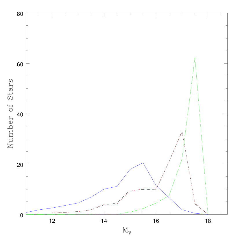
Figure 9: White dwarf luminosity functions for the thin disk (blue solid line), thick disk (red dotted line), stellar halo (black short-dashed line) and dark halo (green long-dashed line). The dark halo luminosity function is created using the 96IMF1 initial mass function parameters.

For the thin disk we assume a metallicity $Z=0.02$ and a uniform star formation rate over the past 11 Gyr. Gilmore (2000) asserts that all thick disk and field halo stars formed within 1–2 Gyr of the onset of star formation, and that there is no detectable age interval between the formation of the field halo stars and the formation of the thick disk. Thus, we model both the thick disk and stellar halo as populations with a uniform star formation rate between 11–12 Gyr with initial metallicity $Z=0.004$. The luminosity functions we generate are shown in Figure (9).

The geometry and stellar content of the thin disk, thick disk and stellar halo described above will be referred to hereafter as our reference model for the known stellar populations.

We begin the simulation by generating a large sample of WD from each component with parameters drawn from models described above. For each simulated WD, we draw a distance along the line of sight, $d<d_{\rm max}$, weighted appropriately according to the density distribution. We choose $d_{\rm max}=5.0$ kpc, a distance large compared to our maximum WD detection limit. We randomly choose space velocities, $(U,V,W)$ from a Gaussian distribution with the appropriate velocity dispersions. We also draw a luminosity, $M_{V}$, according to the component luminosity function. A color, $(V-I)$, is then assigned according to the tracks for a 0.6 $M_{\odot}$ WD from Richer et al. (2000).

Next, we transform variables into the observable quantities. The space velocities are transformed into a radial velocity, $v_{r}$, and velocities in the direction of Galactic longitude and latitude, $(v_{l},v_{b})$, by inverting the following system of equations:

$$U=U_{\odot}+v_{r}\cos{b}\cos{l}-v_{b}\sin{b}\cos{l}-v_{l}\sin{l}~{},$$ (4)

$$V=V_{\odot}+v_{r}\cos{b}\sin{l}-v_{b}\sin{b}\sin{l}+v_{l}\cos{l}~{},$$ (5)

$$W=W_{\odot}+v_{r}\sin{b}+v_{b}\cos{b}~{}.$$ (6)

In these equations, $v_{l}=d~{}\mu_{l}\cos{b}$, $v_{b}=d~{}\mu_{b}$, and $(U_{\odot},V_{\odot},W_{\odot})$ = (10, 5.2, 7.2) km/s is the motion of the Sun with respect to the LSR (Dehnen & Binney, 1998). The transverse velocity on the sky is then $v_{t}=\sqrt{v_{b}^{2}+v_{l}^{2}}$ and the proper motion is given by

$$\left(\frac{\mu}{{}^{\prime\prime}/{\rm y}}\right)=0.211\left(\frac{v_{t}}{{\rm km/s}}\right)\left(\frac{d}{{\rm pc}}\right)^{-1}~{}.$$ (7)

The apparent magnitude is determined by $V=M_{V}+5\log(d/{\rm pc})-5$. Finally, we draw a random number, $r$ between 0.0 and 1.0 and declare the WD to be detectable if $r<\epsilon(V)$ and $\mu_{\rm lim}\sim 0.014^{\prime\prime}/{\rm y}<\mu<\mu_{\rm max}\sim 0.1^{\prime\prime}/{\rm y}$. The function $\epsilon(V)$ indicates our detection efficiency as a function of $V$ magnitude as plotted in Figure 6.

In this way, we create large lists of detectable and non-detectable WD for each component, $k$, from which we may determine the fraction of WD detected in each component, $f_{k}$. We then integrate the number density along our line of sight to determine the number of WD, $K_{k}$, out to $d_{\rm max}=5.0$ kpc. The number of WD from this component we expect to see in the Groth strip is then $\nu_{k}=f_{k}K_{k}$.

As discussed above, the number of expected WD in the Groth strip determined by these simulations scales linearly with our assumptions about the local density of each component. The expected number of WD detections in the Groth strip from known stellar populations scale as

$$\nu_{\rm thin~{}disk}=0.5\left(\frac{n_{0,{\rm thin~{}disk}}}{4.0\times 10^{-3}{\rm pc}^{-3}}\right)~{},$$ (8)

$$\nu_{\rm thick~{}disk}=0.1\left(\frac{n_{0,{\rm thick~{}disk}}}{9.5\times 10^{-5}{\rm pc}^{-3}}\right)~{},$$ (9)

$$\nu_{\rm stellar~{}halo}=0.2\left(\frac{n_{0,{\rm stellar~{}halo}}}{2.2\times 10^{-5}{\rm pc}^{-3}}\right).$$ (10)

The expected number of white dwarfs from known stellar populations is relatively insensitive to our somewhat arbitrary choice of absolute magnitude luminosity functions. The insensitivity is due to the fact that the apparent magnitude luminosity functions of each component are actually determined more by the kinematics of each component then the input absolute magnitude luminosity function. For instance, as the thin disk is the most severely proper motion limited, thin disk WDs are detected at a mean distance much closer to the observer and thus at a much brighter apparent magnitude. Even a drastic adjustment to the input absolute magnitude luminosity function such as giving the thick disk an age of 0–11 Gyr only increases the expected contribution from the thick disk by $\sim 40$%. Alternative disk luminosity functions are discussed in further detail in § 4.4.1.

We expect to detect a total of 0.9 white dwarfs from known stellar populations, if our assumptions about the local white dwarf densities, $n_{0}$, are accurate. Even if we presume a maximal thick disk with a local density scaling to the thin disk of $\sim 5$ (instead of 42), the expected total number of detections is still less then 2. (We note that using the thin disk scale height of Majewski & Siegel (2001) increases the expected number of thin disk detections to 1.9. This is discussed further in § 4.4.1.)

Clearly, our observed sample of 5 white dwarfs is a significant deviation from an expected number of $\sim$1–2. However, the source of the excess of white dwarfs is an open question. Perhaps the simplest explanation is that our estimate of the local white dwarf densities $n_{0}$ are too small for one or more of the known stellar components. Another possibility is that the excess of white dwarfs arises from a fourth component: a dark halo made of ancient white dwarfs. Below, we discuss what we would expect to detect from such a white dwarf component.

4.2 Dark halo WD

Using the same procedure as for the known stellar populations, we estimate the number of WD detections we expect if some fraction, $f_{WD}$, of the Milky Way dark matter halo is made up of white dwarfs. This discussion is motivated by recent microlensing results which suggest that 8%–50% of the dark halo is made up of MACHOs with a most likely MACHO mass between 0.15 and 0.9 $M_{\odot}$ (Alcock et al., 2000).

The Milky Way dark halo density is modeled as

$$n(r)_{\rm dark}=n_{0,{\rm dark~{}halo}}\frac{R_{0}^{2}+a^{2}}{r^{2}+a^{2}}~{},$$ (11)

where $r$ is Galactocentric radius, $R_{0}=8.5$ kpc is the Galactocentric radius of the Sun, and $a=5$ kpc is the halo core radius (Alcock et al., 2000). We use the same velocity dispersions and asymmetric drift as for the stellar halo.

If a substantial portion of the Milky Way dark halo is composed of WD, the initial mass function of this population must be rather sharply peaked in order to avoid chemical evolution constraints. The most plausible initial mass function is peaked at around 2 $M_{\odot}$ (Fields, Freese & Graff, 2000). As an example, we construct a dark halo luminosity function with a uniform star formation rate between 13.0 and 14.0 Gyr with the IMF1 of Chabrier, Segretain & Méra (1996) (hereafter referred to as 96IMF1). This IMF is of the form

$$\phi(m)\propto\exp^{-(\bar{m}/m)^{\beta}}m^{-\alpha},$$ (12)

where $\bar{m}=2.0$, $\beta=2.2$, and $\alpha=5.15$ and peaks around $\sim 1.3M_{\odot}$. We estimate main sequence lifetimes from $Z=0.001$ stars from Girardi et al. (2000) and assume stars instantly become WD on leaving the main sequence. This choice of dark halo luminosity function is also shown in Figure 9. The geometry, age distribution and 96IMF1 initial mass function described above will hereafter be referred to as our reference model for the dark halo.

The number of expected detections from the dark halo scales as

$$\nu_{\rm dark~{}halo}=3.0\left(\frac{n_{0,{\rm dark~{}halo}}}{1.6\times 10^{-3}{\rm pc}^{-3}}\right)$$ (13)

where $n_{0,{\rm dark~{}halo}}=\frac{\rho_{0,{\rm dark~{}halo}}}{\bar{M}_{WD}}\cdot f_{WD}$, and $f_{WD}$ indicates the fraction of the total halo dark matter made up of white dwarfs. We assume a local dark halo mass density $\rho_{0,{\rm dark~{}halo}}=8.0\times 10^{-3}{\rm M_{\odot}~{}pc}^{-3}$, a mean white dwarf mass of 0.5 $M_{\odot}$ and scale our answer to a white dwarf halo fraction of 10% ($f_{WD}=0.10$).

The number of expected dark halo white dwarfs is relatively insensitive to the age of the dark halo in the range 12-14 Gyr. However, $\nu_{\rm dark~{}halo}$ depends critically on the choice of IMF. The IMF described above has the lowest mean initial mass of all the Chabrier IMFs, implying that stars remain on the main sequence longer, and have spent less time cooling as white dwarfs thus giving us the brightest possible dark halo luminosity function. Using IMF2 from Chabrier, Segretain & Méra (1996) (hereafter 96IMF2) which has a slightly higher mean main sequence mass results in a slightly fainter white dwarf luminosity function and decreases the expected number of dark halo white dwarf detections to $\nu_{\rm dark~{}halo}\sim 1$ for a 10% WD halo ($f_{WD}=0.1$).

4.3 Dividing the sample: a maximum likelihood approach

Taken at face value, if we accept the local white dwarf densities from known stellar populations derived in § 4.1 then the total number of WD candidates, $N_{WD}=5$ implies $\nu_{\rm dark~{}halo}=5-0.5-0.1-0.3=4.1$, which by Equation (13) implies a dark halo WD fraction $f_{WD}=0.14$, in line with the microlensing results of Alcock et al. (2000). This interpretation is misleading because our knowledge of the local white dwarf densities and various other model parameters is imperfect. It is not clear whether the excess white dwarfs in our sample arise from an excess of white dwarfs from known stellar populations or whether we must invoke the presence of a fourth dark component to explain our results.

In order to address this question, we must use more information about our sample than simply the total number of observed white dwarfs. Ideally, we would approach the separation of our sample into various components with a purely kinematic approach as in Koopmans & Blandford (2001), removing the most uncertain aspect of our models (age and initial mass functions of each component) from the calculation all together. However, the white dwarfs in our sample are, with one exception, too faint to allow for spectroscopic velocity measurements. They are also potentially too old to allow for a photometric distance calculation as in Oppenheimer et al. (2001) and too distant for parallax measurements. Conversely, samples which are bright enough to allow for distance determinations are not able to exclude the presence of a truly ancient WD dark halo (see e.g. §10 of Koopmans & Blandford (2001)). The existence of an ancient WD halo must be confirmed or denied with a sample in which space velocities cannot be measured, only proper motions.

Proper motions alone will not currently allow any reasonable division of our sample into four separate components. In order to accomplish this we must use all the available information for each white dwarf : $(V,V-I,\vec{\mu})$. Using the component models described above, we may form four dimensional distribution functions in these variables and compare the shape of these distributions with our observed sample. The comparison takes the form of a maximum likelihood analysis in which we determine what linear combination of distributions from each component best fits our observed sample. By introducing the luminosity and color information into the analysis instead of focusing solely on kinematics, our results will depend somewhat on our assumptions about the luminosity functions (especially for division between the stellar and dark halo). Since improved future knowledge about the age and initial mass functions of each component and a larger sample size may reduce this sensitivity, we proceed with a brief investigation of one possible method for separation of a white dwarf sample into various components using only the photometric and astrometric information available for faint objects.

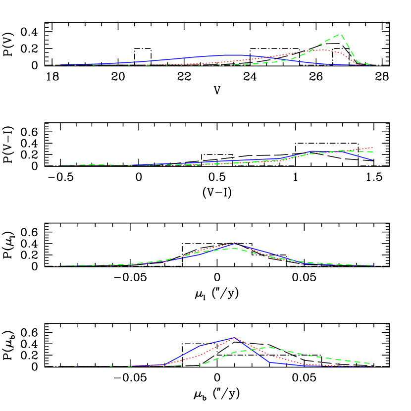
Figure 10: Distributions of detectable WD in the simulations as a function of the observable parameters $(V,V-I,\vec{\mu})$ for various Milky Way components. We show thin disk WD as a blue solid line, thick disk WD as a red dotted line, stellar halo WD as black short-dashed line and the 96IMF1 dark halo WD as a green long-dashed line. We also overplot the distribution of observed WD from the 5 WD sample as a black dot-dashed histogram.

In Figure 10, we show the one dimensional projections of the distribution functions $P(V,V-I,\vec{\mu})$ for detectable WD in our simulations from the thin disk (blue), thick disk (red), stellar halo (black) and dark halo (green). The parameters for each Galactic component are those of our reference model described in § 4.1 and § 4.2. We also show the distribution of the observed 5 WD sample as a dashed black histogram. All curves have been normalized such that the total area under the curve is unity. The proper motion vector has been divided into two components, $\mu_{l}$ and $\mu_{b}$, the proper motion in the direction of increasing galactic latitude and longitude, respectively.

The curves in Figure 10 are the one dimensional projection of a four dimensional cube, $P_{k}(V,V-I,\vec{\mu})$, in which each element of the cube, $i$, holds the probability that a WD from each component $k$ will be detected within some small volume element centered about $(V,V-I,\vec{\mu})$. The cube is normalized such that the sum over all cells is unity,

$$\sum_{i}P_{k}(V_{i},V_{i}-I_{i},\vec{\mu}_{i})=1.0~{}.$$ (14)

If the number of WD drawn from a given component is $\nu_{k}$, then the occupation number of cell $i$ is

$$\lambda_{ik}=\nu_{k}~{}P_{k}(V_{i},V_{i}-I_{i},\vec{\mu_{i}})~{}.$$ (15)

If we sum the four dimensional cubes over all components, $k$, multiplied by the appropriate coefficient, $\nu_{k}$, we create the distribution function of white dwarfs for the entire galaxy. The occupation number of a cell in this cube is thus

$$\lambda_{i}=\sum_{k}\nu_{k}P_{k}(V_{i},V_{i}-I_{i},\vec{\mu_{i}})~{}.$$ (16)

We assume that the cell size is small enough that $\lambda_{i}<<1.0$ and that in a given sample of observed WD, a cell will contain at most one white dwarf. A sample of observed WD then defines two sets of cells: the set F whose cells are filled with the observed WD, and the set E whose cells are empty. Given a defined set F of observed WD, the likelihood of a configuration with a given set of coefficients $\{\nu_{k}\}$ is

$$L=L(\nu_{k})=\left[\sum_{i\in F}\lambda_{i}\right]\left[\sum_{i\in E}(1.0-\lambda_{i})\right]~{}.$$ (17)

Maximizing over the four dimensional space, we find that the maximum likelihood occurs at ($\nu_{\rm thin~{}disk}$, $\nu_{\rm thick~{}disk}$, $\nu_{\rm stellar~{}halo}$, $\nu_{\rm dark~{}halo}$)$=(3.0,0.0,0.0,2.0)$ $\equiv(w_{0},x_{0},y_{0},z_{0})$.

In Figure (11), we show a two dimensional projection of the likelihood space where we sum over the thin and thick disk to form a “disk” component, and sum over the stellar and dark halo to form a “halo” component. That is, for each point in this two dimensional surface we average all points in the four dimensional likelihood surface where $(\nu_{\rm thin~{}disk}+\nu_{\rm thick~{}disk}=\nu_{\rm disk})$ and $(\nu_{\rm stellar~{}halo}+\nu_{\rm dark~{}halo}=\nu_{\rm halo})$. The vertical dashed line shows the number of expected disk white dwarfs assuming the canonical number densities of Equations 8 and 9. The horizontal dashed line shows the number of expected stellar halo white dwarfs with the canonical number density of Equation 10. Our most likely point in this projection falls at $\nu_{\rm disk}=3.75$, $\nu_{\rm halo}=1.5$, several orders of magnitude in likelihood from the intersection of the two canonical values. This plot emphasizes that we see too many WD in all components, disk and halo.

We calculate statistical error bars on the set of $\nu_{k}$ in the four dimensional maximum likelihood analysis using Bayes’ Theorem:

$$P(w,x,y,z)=P(w,x,y,z|\{w_{0},x_{0},y_{0},z_{0}\}_{\rm actual})$$ (18)

$$~{}~{}~{}~{}~{}~{}~{}~{}~{}~{}~{}~{}~{}~{}=\frac{P(w_{0},x_{0},y_{0},z_{0}|w,x,y,z)}{\sum_{w,x,y,z}P(w_{0},x_{0},y_{0},z_{0}|w,x,y,z)}$$ (19)

The term on the left hand side is the probability of finding the maximum likelihood value at $(\nu_{\rm thin~{}disk},\nu_{\rm thick~{}disk},\nu_{\rm stellar~{}halo},\nu_{\rm dark~{}halo})=(w,x,y,z)$ if the actual values are ($\nu_{\rm thin~{}disk}$, $\nu_{\rm thick~{}disk}$, $\nu_{\rm stellar~{}halo}$, $\nu_{\rm dark~{}halo}$) $=(w_{0},x_{0},y_{0},z_{0}0)$. The terms on the right hand side are computed in a monte carlo fashion. To compute $P(w_{0},x_{0},y_{0},z_{0}|w,x,y,z)$ we assume that ($\nu_{\rm thin~{}disk}$, $\nu_{\rm thick~{}disk}$, $\nu_{\rm stellar~{}halo}$, $\nu_{\rm dark~{}halo}$) $=(w,x,y,z)$ are the correct parameters and form 2000 simulated data sets drawn from the co-added four dimensional distribution function with these coefficients. For each simulated data set we compute the maximum likelihood point. $P(w_{0},x_{0},y_{0},z_{0}|w,x,y,z)$ is then the fraction of the simulated data sets with input coefficients $(w,x,y,z)$ whose maximum likelihood point falls within some small volume of $(w_{0},x_{0},y_{0},z_{0})$.

We have now created a four dimensional probability distribution function $P(w,x,y,z)$ in parameter space. We reduce this to more intuitive one dimensional functions by summing over the remaining variables, eg.

$$P(w)=\frac{\sum_{x,y,z}P(w_{0},x_{0},y_{0},z_{0}|w,x,y,z)}{\sum_{w,x,y,z}P(w_{0},x_{0},y_{0},z_{0}|w,x,y,z)}~{}.$$ (20)

The resulting probability distribution function for $\nu_{\rm thin~{}disk},\nu_{\rm thick~{}disk},\nu_{\rm stellar~{}halo}$ and $\nu_{\rm dark~{}halo}$ are shown in Figure 14. The curves have been arbitrarily renormalized such that the total area under each curve is 1.0. We compute $1\sigma$ error bars as the smallest distance which encloses 69% of the area under the curve, giving $\nu_{\rm thin~{}disk}=3.0^{+0.9}_{-0.8}$, $\nu_{\rm thick~{}disk}=0.0^{+0.8}$, $\nu_{\rm stellar~{}halo}=0.0^{+0.8}$ and $\nu_{\rm dark~{}halo}=2.0^{+0.8}_{-0.8}$. The error bar calculation is extremely computationally intensive and we estimate that the sums expressed in Equation 20 are converged to $\sim$5%. We devoted the available CPU cycles in such a manner that the peaks of the probability distribution functions in Figure 14 were calculated to greater accuracy then the wings. Further computation would serve to raise the wings slightly and thus increase the error bars slightly.

These values may now be used to work backwards to observed values for the local WD number densities using the scaling relations in Equations (8–10) and (13). With the error bars calculated as described above, our final analysis yields $n_{0,{\rm thin~{}disk}}=2.4^{+0.7}_{-0.6}\times 10^{-2}$ pc^-3, $n_{0,{\rm thick~{}disk}}=0.0^{+7.6}\times 10^{-4}$ pc^-3, $n_{0,{\rm stellar~{}halo}}=0.0^{+7.7}\times 10^{-5}$ pc^-3, $n_{0,{\rm dark~{}halo}}=1.0^{+0.4}_{-0.4}\times 10^{-3}$ pc^-3.

Given this model of the dark halo using the 96IMF1 dark halo luminosity function, our results imply the presence of a $\sim 7$% white dwarf dark halo (with substantial statistical error bars) and an excess of thin disk white dwarfs. The thin disk contribution is $\sim 6$ times the canonical value. However, the statistical error bars on the thin disk contribution are quite large - even with the error bars projected into one dimension, we are still less then 2.5$\sigma$ from the canonical value. It is also possible that this spuriously high value arises because our model of the thin disk is wrong. We discuss the possibility of a thin disk with a much larger scale height (Majewski & Siegel, 2001) in § 4.4.1.

4.4 Alternative Galactic models

We define in § 4.1 and § 4.2 one possible model for our Galaxy. However, all parameters in this model are uncertain to some extent. The kinematics are uncertain for stars as distant as our sample and the age and initial mass functions chosen above are certainly disputable. In this section we explore alternative and equally credible models of the Galaxy. Although the modifications we explore below do change our results somewhat, our solution always returns roughly $\sim 3$ disk WD and $\sim 2$ halo WD. Minor modifications to our models and procedure shift the disk WD around between the thin and thick disk and the halo WD between the stellar and dark halo.

In the following examples, we do not recompute statistical error bars as this exercise is prohibitively computationally expensive. We include this section to emphasize that our statistical error bars of $\sim 30$% are actually small compared to the systematic uncertainties in our models.

4.4.1 Alternative disk models

Our models for the thin and thick disk include information about both the geometry (density profiles, scale heights, velocity dispersions) and stellar content (age distribution, initial mass function) of each component. We find that the division of our sample between the thin and thick disks is insensitive to the age distributions of the disk components and depends mainly on the kinematics.

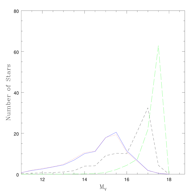
Figure 12: White dwarf absolute magnitude luminosity functions for each Galactic component as in Figure 9 except with a young thick disk of age 0–11 Gyr.

In § 4.3 we describe the results of our maximum likelihood analysis using our reference model which has a thin disk of age 0–11 Gyr and a thick disk of age 11–12 Gyr, modelling the thick disk as an old population formed in a single burst. At the opposite extreme, we may consider a thick disk whose age distribution is identical to that of the thin disk, uniform star formation from 0–11 Gyr ago. This gives a thick disk absolute luminosity function nearly identical to that of the thin disk, shown in Figure 12. (The small variation between the thin and thick disk luminosity function is due to our different metallicity assumptions, Z=0.02 for the thin disk and Z=0.004 for the thick disk.)

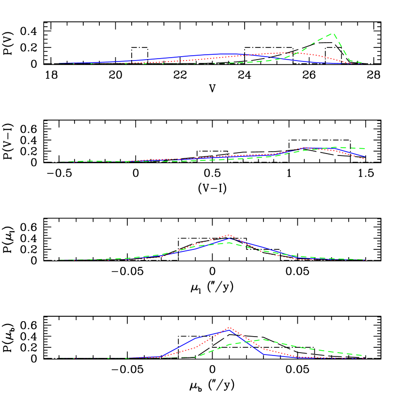
Figure 13: Distributions of detectable WD in the simulations as a function of the observable parameters $(V,V-I,\vec{\mu})$ for various Milky Way components as in Figure 10 but with the young thick disk luminosity function of Figure 12.

However, despite the near identical nature of the thin and thick disk absolute magnitude luminosity functions in Figure 12, the resulting apparent magnitude luminosity functions (shown in Figure 13) are quite different. Conversely, despite the great difference in absolute magnitude luminosity function between the 0–11 Gyr thick disk in Figure 12 and the 11–12 Gyr thick disk in Figure 9, the apparent magnitude luminosity functions of the thick disks in Figures 10 and 13 are very similar.

The apparent magnitude luminosity functions of the 0–11 Gyr and 11–12 Gyr thick disks remain similar because the apparent magnitude luminosity functions are more sensitive to the kinematics than to the input absolute magnitude functions. The thin disk has smaller velocity dispersions and is, therefore, more severely proper motion limited than the thick. Thus, the mean distance at which we detect a thin disk WD is much smaller than the mean distance at which we detect a thick disk WD. From this it follows that the detectable thin disk WD are also brighter in apparent magnitude.

The kinematics dominate the difference in apparent magnitude luminosity functions of the thin and thick disks to such an extent that a by-eye comparison of the thick disk distributions in Figures 10 and 13 shows that the difference in observable quantities between a thick disk of age 11–12 Gyr and a thick disk of age 0–11 Gyr is slight. Performing our maximum likelihood analysis with the 0–11 Gyr thick disk and the other components as in our reference model, we find, $n_{0,{\rm thin~{}disk}}=2.4\times 10^{-2}$ pc^-3,$n_{0,{\rm thick~{}disk}}=0.0$ pc^-3, $n_{0,{\rm stellar~{}halo}}=0.0$ pc^-3, $n_{0,{\rm dark~{}halo}}=1.0\times 10^{-3}$ pc^-3, identical to our results with the old, burst model for the thick disk.

We also explore the possibility that our model for the thin disk is in error. Recent results by Majewski & Siegel (2001) suggest that the canonical thin disk scale height is too small. They suggest a scale height of 400-600 pc for old thin disk populations. If their assertion is correct, the effect on our simulations is substantial as the great majority of our WD candidates are detected at least one scale scaleheight above the plane. This effect would be evident in our sample as an overabundance of thin disk white dwarfs compared to what we expect to see with a thin disk with a scaleheight of 300 pc.

We model the Majewski & Siegel (2001) thin disk as a disk with scaleheight 500 pc, $5/3$ larger then the canonical value. To maintain consistency with the Boltzman equations, we scale the thin disk velocity dispersions by the same factor of $5/3$ (Binney & Tremaine, 1998). This model gives an expected number of thin disk white dwarf detections

$$\nu_{\rm thin~{}disk}=1.9\left(\frac{n_{0,{\rm thin~{}disk}}}{4.0\times 10^{-3}{\rm pc}^{-3}}\right)~{},$$ (21)

and the maximum likelihood analysis gives $n_{0,{\rm thin~{}disk}}=6.2\times 10^{-3}$ pc^-3, $n_{0,{\rm thick~{}disk}}=0.0$ pc^-3, $n_{0,{\rm stellar~{}halo}}=0.0$ pc^-3, and $n_{0,{\rm dark~{}halo}}=1.0\times 10^{-3}$ pc^-3 with the other components modelled as in our reference model. Assuming a statistical error bar of $\sim 30$%, the Majewski & Siegel (2001) thick disk scale height lowers our local thin disk density to within $\sim 1$ sigma of the canonical value.

4.4.2 Alternative halo models

Since the stellar halo and dark halo in our models have similar density profiles and identical kinematics, the separation of the halo signal into the stellar halo and dark halo depends entirely on our assumptions about their stellar content. In §4.3 we assumed a stellar halo of age 11–12 Gyr with a Saltpeter initial mass function and a dark halo of age 13–14 Gyr with the 96IMF1 initial mass function. This led to a result suggesting a $\sim 7$% white dwarf dark halo.

However, this result depends entirely on our choice of initial mass function for the dark halo. Any assumption which makes the dark halo luminosity function any fainter will shift the halo signal from the dark halo to the stellar halo. For instance, a switch to the 96IMF2 initial mass function gives a most likely answer of $\nu_{\rm thin~{}disk}=3.0$, $\nu_{\rm thick~{}disk}=0.0$, $\nu_{\rm stellar~{}halo}=2.0$ and $\nu_{\rm dark~{}halo}=0.0$, or $n_{0,{\rm thin~{}disk}}=2.4\times 10^{-2}$ pc^-3,$n_{0,{\rm thick~{}disk}}=0.0$ pc^-3, $n_{0,{\rm stellar~{}halo}}=2.2\times 10^{-4}$ pc^-3, $n_{0,{\rm dark~{}halo}}=0.0$ pc^-3. The small change in initial mass function removes all signal from the dark halo and gives results for the stellar halo within 1$\sigma$ of Koopmans & Blandford (2001).

We note that even if our halo signal belongs in the stellar halo instead of the dark halo, it still implies a halo white dwarf density $\sim 10$ times higher then expected from halo field star counts (Gould, Flynn & Bahcall, 1998) and still implies that $\sim 1.5$% of the halo mass is in white dwarfs. These estimates are consistent with the results of Oppenheimer et al. (2001).

4.4.3 Constrained models

In this section, we consider two constrained models in which we fix the value of the local density for certain components and fit for the local density of the remaining components. Again, we do not recompute statistical error bars for the examples in this section. All examples in this section use the reference models for each Galactic component described in § 4.1 and 4.2.

First, we consider a solution in which we constrain the thin disk contribution to the expected value of $\nu_{\rm thin~{}disk}=0.5$ (or $n_{0,{\rm thin~{}disk}}=4.0\times 10^{-3}$ pc^-3) as given by Equation 8. Unsurprisingly, most of the remaining disk signal shifts into the thick disk, giving $n_{0,{\rm thick~{}disk}}=1.9\times 10^{-3}$ pc^-3, $n_{0,{\rm stellar~{}halo}}=0.0$ pc^-3, $n_{0,{\rm dark~{}halo}}=8.2\times 10^{-4}$ pc^-3.

Next, we performed an experiment in which we adopt the Koopmans & Blandford (2001) approach and first remove the thin disk contribution by hand and fit only for contributions from the thick disk and a stellar halo. In this approach, we remove our brightest candidate (WD3) and fit only for the thick disk and stellar halo. We find $n_{0,{\rm thick~{}disk}}=3.2\times 10^{-3}$ pc${}^{-}3$ and $n_{0,{\rm stellar~{}halo}}=6.1\times 10^{-5}$ pc^-5. Allowing for a statistical error bar in our measurements of $\sim$30%, this is within 1.5$\sigma$ of their results. We also note that the Koopmans & Blandford (2001) point in Figure 11 falls within $\sim 1.5\sigma$ of our most likely point.

4.5 Alternative WD samples

A final source of uncertainty in our analysis is the observed sample of WD itself. As discussed in §3.1 there is some possibility that our WD sample should include the two marginal candidates WD6 and WD7, giving us a 7 WD sample. Taking the opposite approach we might conclude that all our faint candidates should be excluded and include only WD1, WD3 and WD4, giving a 3 WD sample.

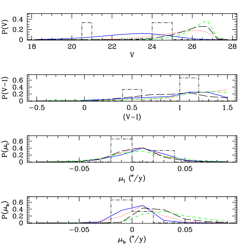
Figure 15: Distributions of detectable WD for various galactic components as described in Figure 10. We overplot the distribution of observed WD in the 3 WD sample as a dashed black histogram.

In Figure 15 we compare the 3 WD sample to the one dimensional distribution functions of our reference model using the 96IMF1 dark halo luminosity function. This sample gives $(\nu_{\rm thin~{}disk}$, $\nu_{\rm thick~{}disk},$ $\nu_{\rm stellar~{}halo}$, $\nu_{\rm dark~{}halo})$ $=(3.0,0.0,0.0,0.0)$ for a thin disk density $n_{0,{\rm thin~{}disk}}=2.4^{+0.7}_{-0.6}\times 10^{-2}$ pc^-3.

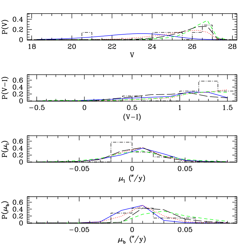
Figure 16: Distributions of detectable WD for various galactic components as described in Figure 10. We overplot the distribution of observed WD in the 7 WD sample as a dashed black histogram.

In Figure 16 we compare the 7 WD sample to the one dimensional distribution functions. This sample gives $(\nu_{\rm thin~{}disk},\nu_{\rm thick~{}disk},\nu_{\rm stellar~{}halo},\nu_{\rm dark~{}halo})=(2.0,3.5,0.0,1.7)$. The thin disk contribution is lower for the larger sample because the outlier at $V=20.7$ is less significant. That is, in one dimension, this outlier accounts for only 14% of the area under the observed WD $V$ magnitude histogram instead of 20% or 33%. The maximum likelihood analysis can put less “power” in the thin disk and still fit this outlier. The extra power in this analysis falls entirely into the thick disk. The 7 WD sample gives densities of $n_{0,{\rm thin~{}disk}}=1.5\times 10^{-2}$ pc^-3, $n_{0,{\rm thick~{}disk}}=3.3\times 10^{-3}$ pc^-3, $n_{0,{\rm stellar~{}halo}}=0.0$ pc^-3, $n_{0,{\rm dark~{}halo}}=9.6\times 10^{-5}$ pc^-3, or a 6% WD halo.

5 Discussion

Koopmans & Blandford (2001) and Reid, Sahu & Hawley (2001) demonstrate that the Oppenheimer et al. (2001) results do not necessarily imply the presence of a substantial white dwarf dark matter halo. They also note that due to the color turnoff of ancient white dwarfs a survey with such a bright limiting magnitude cannot exclude the presence of an ancient white dwarf halo of age $\gg 10$ Gyr. To exclude an ancient halo requires a survey with a substantially fainter limiting magnitude, such as this one.

For faint or ancient white dwarfs, spectroscopic velocities are not available, parallax measurements cannot be made and photometric distance relations calibrated at bright magnitudes are potentially unreliable. Therefore, the division of a faint white dwarf sample into disk and halo contributions must be done without true kinematic (velocity) information.

In this work, we have explored such a statistical separation using only the directly observable quantities of the five high proper motion white dwarf candidates detected in a second WFPC2 epoch of the Groth-Westphal strip. The small sample size and our imperfect knowledge of the characteristics of the putative white dwarf dark halo lead to possible large systematic errors in our analysis. Using the 96IMF1 dark halo gives a 7% white dwarf halo and $n_{0,{\rm thin~{}disk}}=2.4^{+0.5}_{-0.4}\times 10^{-2}$ pc^-2, a gross excess of thin disk white dwarfs. However, we explore several alternative Galactic models which demonstrate that uncertainties in our models lead to possible systematic errors which may be larger then the quoted statistical errors.

For instance, the thin disk local density can be lowered four-fold and brought to within $1$ sigma of the canonical value by assuming the larger thin disk scale height suggested by Majewski & Siegel (2001). Also, if we assume a slightly different dark halo initial mass function, the halo signal shifts to the stellar halo where it implies a local stellar halo white dwarf density of $n_{0,{\rm stellar~{}halo}}\sim 2.2\times 10^{-4}$, about 10 times higher then the canonical value and similar to the results reported by Oppenheimer et al. (2001).

The use of external constraints also affects our results. If we constrain the thin disk contribution to the canonical value, or attempt to remove the thin disk contribution by hand (as in Koopmans & Blandford (2001)), the disk signal shifts into the thick disk, giving $n_{0,{\rm thick~{}disk}}\sim 3\times 10^{-3}$ pc^-3. This elevated thick disk density is similar to the results of Koopmans & Blandford (2001).

However, regardless of the details of our models, we always find $\sim 3$ disk white dwarfs and $\sim 2$ halo white dwarfs, a clear excess above the $\sim$1–2 total detections expected from known stellar populations. We are unable to definitely determine the source of the excess signal, but its existence seems clear. We summarize the local densities found in our various calculations in Table 3.

We note that the ages, abundances and kinematics of the known stellar populations of our Galaxy are still a source of lively debate. We have attempted to highlight how our results depend on our assumptions about these quantities in §4.4. Attempts to more precisely determine the properties of the various components of our Galaxy will benefit from surveys with very precise astrometry.

Both our results and those of Oppenheimer et al. (2001) are intriguing and together explore the two extremes of survey philosophies: bright limiting magnitude with many objects and faint limiting magnitude with few objects. The Oppenheimer et al. (2001) sample is bright enough to be able to employ photometric distance calibrations, however, fainter surveys necessary to truly exclude or confirm the dark white dwarf halo must employ an approach more similar to ours. Future improved knowledge of the input model characteristics and a faint sample with more objects may reduce the model dependencies which hamper our conclusions.

Figure 2: Residuals in the X coordinate, $\Delta X$, to the transformations between epochs. The top two panels show $\Delta X$ plotted versus the X and Y position on the chip. The third panel shows the residuals as a function of $V$ magnitude. The bottom panel shows the residuals as a function of radius from the distortion center of the chip. Residals are plotted in units of arcseconds.

Figure 3: As in Figure 2 but for residuals in the Y coordinate, $\Delta Y$.

Figure 4: Vector plot of the residuals to the transformations as a function of position on the chip. The residuals are multiplied by a factor of 40 to improve visibility.

Figure 5: Vector proper motions for the high proper motion objects as a function of position on the WFPC2 chip. The proper motions are multiplied by a factor of 20 to improve visibility.

Figure 6: The fraction of objects detected as a function of V magnitude, $\epsilon(V)$ and proper motion, $\epsilon(\mu)$. Results are averaged over all Groth strip fields.

Figure 11: Likelihood contours collapsed into two dimensions. For each point we average all points in the four dimensional likelihood surface where $(\nu_{\rm thin~{}disk}+\nu_{\rm thick~{}disk}=\nu_{\rm disk})$ and $(\nu_{\rm stellar~{}halo}+\nu_{\rm dark~{}halo}=\nu_{\rm halo})$. The vertical dashed line shows the number of expected disk white dwarfs with the canonical number density of a Legget, Ruiz & Bergeron (1998) thin disk plus a thick disk scaled by $n_{0,{\rm thin}}/n_{0,{\rm thick}}=42$ as in Alcock et al. (2000). The horizontal dashed line shows the number of expected stellar halo white dwarfs with the canonical number density of Gould, Flynn & Bahcall (1998). Our most likely point falls at $\nu_{\rm disk}=3.75$, $\nu_{\rm halo}=1.5$, several orders of magnitude in likelihood from the intersection of the two canonical values. We also mark with an X the number of expected white dwarfs assuming the Koopmans & Blandford (2001) number densities with an additional contribution from a Legget, Ruiz & Bergeron (1998) thin disk and assuming that the Koopmans & Blandford (2001) white dwarfs with halo kinematics belong to the stellar halo.

Figure 14: The probability distribution functions for each parameter, ($\nu_{\rm thin~{}disk}$, $\nu_{\rm thick~{}disk}$, $\nu_{\rm stellar~{}halo}$, $\nu_{\rm dark~{}halo}$) determined in our maximum likelihood analysis for the 5 WD sample and the 96IMF1 dark halo IMF.

Table 1: Observations

R.A. (2000)	Decl. (2000)	Epoch 1 (MJD)	Epoch 2 (MJD)
14:15:21	52:02:59	49426.1	51978.7
14:15:27	52:04:10	49419.9	51979.4
14:15:33	52:05:20	49419.7	51991.8
14:15:40	52:06:30	49419.4	51988.8
14:15:46	52:07:40	49451.4	51984.0
14:15:53	52:08:51	49426.6	51988.9
14:15:59	52:10:01	49420.9	51978.0
14:16:06	52:11:11	49428.8	51978.9
14:16:12	52:12:21	49420.6	51990.1
14:16:19	52:13:31	49422.0	51986.1
14:16:25	52:14:41	49428.5	51978.3
14:16:31	52:15:51	49428.0	51983.0
14:16:38	52:17:01	49425.8	51977.1
14:17:10	52:22:51	49418.9	51993.0
14:17:17	52:24:01	49418.6	51994.8
14:17:56	52:31:00	49422.8	51987.9
14:18:03	52:32:10	49427.4	51984.2

Table 2: White Dwarf Candidates

Candidate	RA	DEC	$\mu$	$\mu_{l}$	$\mu_{b}$	$V$	$V-I$	$t_{\rm cool}$ (Gyr)	$M_{V}$	$d$(pc)	$v_{t}$(km/s)
WD1	14:15:54.5	52:09:16.8	0.020	-0.038	-0.008	24.81	1.09	$3.7^{+3.2}_{-3.1}$	$14.9^{+0.9}_{-0.5}$	$940^{+370}_{-600}$	$90^{+20}_{-25}$
								$11.4^{+0.1}_{-0.7}$	$17.4^{+0.2}_{-0.3}$	$310^{+50}_{-40}$	$29^{+5}_{-4}$
WD2	14:16:02.0	52:10:44.5	0.029	0.035	0.024	26.90	1.38	$7.9^{+2.0}_{-3.3}$	$16.1^{+0.8}_{-0.8}$	$1460^{+800}_{-530}$	$205^{+112}_{-74}$
								$10.5^{+0.6}_{-0.4}$	$17.1^{+0.2}_{-0.1}$	$910^{+130}_{-120}$	$128^{+18}_{-18}$
WD3	14:16:13.3	52:11:38.6	0.032	0.053	0.018	20.67	0.55	$1.2^{+0.6}_{-0.5}$	$13.4^{+0.6}_{-0.7}$	$290^{+100}_{-85}$	$44^{+24}_{-13}$
								$12.5^{+0.5}_{-0.3}$	$17.6^{+0.1}_{-0.1}$	$40^{+5}_{-5}$	$6^{+1}_{-1}$
WD4	14:16:12.8	52:12:12.4	0.019	-0.038	-0.004	24.02	1.02	$3.2^{+3.5}_{-1.1}$	$14.7^{+0.8}_{-0.6}$	$720^{+290}_{-250}$	$66^{+20}_{-23}$
								$11.6^{+0.5}_{-0.6}$	$17.4^{+0.2}_{-0.2}$	$210^{+40}_{-30}$	$19^{+3}_{-2}$
WD5	14:15:25.8	52:04:16.1	0.051	0.021	0.050	25.49	1.28	$6.6^{+3.3}_{-3.1}$	$15.7^{+1.1}_{-0.9}$	$900^{+500}_{-410}$	$217^{+126}_{-91}$
								$10.8^{+0.7}_{-0.7}$	$17.2^{+0.2}_{-0.2}$	$460^{+80}_{-40}$	$111^{+20}_{-18}$
WD6∗	14:15:39.8	52:04:48.3	0.016	-0.021	0.012	26.33	1.62	$10.0^{+0.3}_{-1.8}$	$16.9^{+0.1}_{-0.7}$	$770^{+370}_{-110}$	$57^{+29}_{-7}$
WD7∗	14:18:25.8	52:04:16.1	0.019	-0.038	0.003	26.93	1.60	$10.0^{0.1}_{-2.0}$	$16.9^{+0.1}_{-0.8}$	$1000^{+560}_{-130}$	$91^{+49}_{14}$

Note. — ^∗ indicates marginal white dwarf candidates as discussed in §3.1. Proper motions in the plane of the sky, $\mu$, in the direction of increasing Galactic longtitude $\mu_{l}$, and latitude, $\mu_{b}$, are given in units of ^′′/yr. We estimate an uncertainty on all $V$ magnitudes of 0.15 mag and an uncertainty on all $(V-I)$ colors of 0.20 mag. The error in proper motion, $\mu$ is 0.004 ${\prime\prime}$/yr. Error bars are calculated for derived quantities by finding the maximum and minimum values attainable within 1 unit of photometric uncertainty.

Table 3: Local white dwarf densities

Source	$n_{0,{\rm thin~{}disk}}$	$n_{0,{\rm thick~{}disk}}$	$n_{0,{\rm stellar~{}halo}}$	$n_{0,{\rm dark~{}halo}}$
Canonical Values	$4.0\times 10^{-3}$	$9.5\times 10^{-5}$	$2.2\times 10^{-5}$	$0.0$
Koopmans & Blandford (2001)	$\cdots$	$1.8^{+0.5}_{-0.5}\times 10^{-3}$	$1.1^{2.1}_{-0.7}\times 10^{-4}$	$\cdots$
Reference Model (§4.3)	$2.4^{+0.7}_{-0.6}\times 10^{-3}$	$0.0^{+7.6}\times 10^{-4}$	$0.0^{+7.7}\times 10^{-5}$	$1.0^{+0.4}_{-0.4}\times 10^{-3}$
Increased Thin Disk Scale Height(§4.4.1)	$6.2\times 10^{-3}$	$0.0$	$0.0$	$1.0\times 10^{-3}$
96IMF2 Dark Halo (§4.4.2)	$2.4\times 10^{-3}$	$0.0$	$2.2\times 10^{-4}$	$0.0$
Contrained Thin Disk (§4.4.3)	$4.0\times 10^{-3}$	$1.9\times 10^{-3}$	$0.0$	$8.2\times 10^{-4}$

Note. — All densities are given in units of $M_{\odot}$ pc^-3. The known stellar populations assume a mean white dwarf mass of 0.6 $M_{\odot}$. The dark halo assumes a mean white dwarf mass of 0.5 $M_{\odot}$. The Koopmans & Blandford (2001) work does not distinguish between a stellar and a dark halo. We have listed their halo density under the $n_{0,{\rm stellar~{}halo}}$ column, but it could also be listed under $n_{0,{\rm dark~{}halo}}$.

References

- Alcock et al. (1997) Alcock, C., et al. 1997, ApJ, 486, 697
- Alcock et al. (2000) Alcock, C., et al. 2000, ApJ, 542, 281
- Baraffe et al. (1998) Baraffe, I., Chabrier, G., Allard, F., & Hauschildt, P.H. 1998, A&A, 337, 403
- Bergeron, Ruiz & Leggett (1997) Bergeron, P., Ruiz, M.-T., Legget, S.K. 1997, ApJS, 108, 339
- Bertelli et al. (1994) Bertelli, G., Bressan, A., Chiosi, C., Fagotto, F., & Nasi, E. 1994, A&AS, 106, 275
- Bertin & Arnouts (1996) Bertin, E. & Arnouts, S. 1996, A&A, 117, 393
- Binney & Tremaine (1998) Binney, J. & Tremaine, S. 1998, Galactic Astronomy (Princeton; Princeton Univ. Press)
- Carr (1994) Carr, B. 1994,ARA&A, 32, 531
- Cassisi et al. (2000) Cassisi, S., Castellani, V., Ciarcelluti, P., Piotto, G., Zoccali, M. 2000, MNRAS, 315, 679
- Chabrier, Segretain & Méra (1996) Chabrier, G., Segretain, L, & Mera, D. 1996, ApJ, 468, L21
- Chabrier (1999) Chabrier, G. 1999, ApJ, 513, L103
- Chiba & Beers (2000) Chiba, M. & Beers, T.C. 2000, AJ, 119, 2843
- Davies (2001) Davies, M.B., King, A.R. & Ritter, H. 2001, astro-ph/0107456
- Dehnen & Binney (1998) Dehnen, W., & Binney, J. 1998, MNRAS, 298, 387
- Dolphin (2000) Dolphin, A.E. 2000, PASP, 112, 1383
- Fields, Freese & Graff (2000) Fields, B.D., Freese, K., Graff, D.S. 2000, ApJ, 534, 265
- Gilmore (2000) Gilmore, G. 2000, Galaxy Disks and Disk Galaxies, ASP Conference Series, Vol.3, astro-ph/0011450
- Girardi et al. (2000) Girardi, L., Bressan, A., Bertelli, G.& Chiosi, C. 2000, A&A, 141, 371
- Gould, Bahcall & Flynn (1997) Gould, A., Bahcall, J.N., & Flynn, C. 1997, ApJ, 482, 913
- Gould, Flynn & Bahcall (1998) Gould, A., Flynn, C., Bahcall, J.N. 1998, ApJ, 503, 798
- Groth et al. (1994) Groth, E.J., Kristian, J.A., Lynds, R., O’Neil, E.J., Balsano, R., Rhodes, J., & the WFPC-1 IDT. 1994, BAAS, 26, 1403
- Giudice, Mollerach & Rollet (1994) Giudice, G.F., Mollerach, S., & Roulet, E. 1994, Phys. Rev. D, 50, 2406
- Hansen (1998) Hansen, B.M.S. 1998, Nature, 394, 860
- Hansen (1999) Hansen, B.M.S. 1999, ApJ, 520, 680
- Hansen (2001) Hansen, B.M.S. 2001, ApJ, 558, L39
- Holtzman et al. (1995a) Holtzman, J., et al. 1995, PASP, 107,156
- Holtzman et al. (1995b) Holtzman, J., Burrows, C.J., Casertano, S., Hester, J., Trauger, J.T., Watson, A.M., & Worthey, G. 1995, PASP, 107, 1065
- Ibata et al. (1999) Ibata, R.A., Richer, H.B., Gilliland, R.L., & Scott, D. 1999, ApJ, 524, L95
- Knox, Hawkins & Hambly (1999) Knox, R.A., Hawkins, M.R.S, & Hambly, N.C. 1999, MNRAS, 306, 736
- Kochanek (1996) Kochanek, C. 1996, ApJ, 457, 228