Faraday Rotation Effect of Intracluster Magnetic Field on Cosmic Microwave Background Polarization

Abstract

The observed magnetic field of microgauss strength in clusters of galaxies should induce the Faraday rotation effect on the linearly polarized cosmic microwave background (CMB) radiation when the CMB radiation propagates through a cluster at low redshift. The Faraday rotation arises from combined contributions of the magnetic field strength, the electron density, the cluster size, and the characteristic scale of the magnetic field along the line of sight. Employing the Press-Schechter prescription for the cluster abundance under the cold dark matter (CDM) scenario and a plausible isothermal $\beta$-model for the gas distribution, we compute angular power spectra of the CMB polarization fields including the Faraday rotation mixing effect under the simple assumption of uniform magnetic field configuration across a cluster. As a result, we find that a parity-odd $B$-type polarization pattern is statistically generated on the observed sky, even when the primary polarization only contains the parity-even $E$-mode component, such as in the case of pure scalar perturbations. The generated $B$-type polarization has a peak with amplitude of $\sim 0.1~{}\mu{\rm K}(B_{0}/0.1~{}\mu{\rm G})(\nu_{0}/10~{}{\rm GHz})^{-2}$ at angular scales of $l\approx 1000$ for the currently favored adiabatic $\Lambda$CDM model. This result also implies that, if the magnetic field has a $0.5~{}\mu{\rm G}$ strength and we observe at lower frequencies such as $\nu_{0}\lower 2.15277pt\hbox{$\;\buildrel<\over{\sim}\;$}5~{}{\rm GHz}$, the secondary signal due to the Faraday rotation effect could be comparable to the magnitude of the primary polarization. The frequency dependence of the Faraday rotation can be then used to discriminate the effect from primary and other secondary signals on the CMB polarizations. Our results therefore offer a new empirical opportunity to measure or constrain the intracluster magnetic field in the average sense, combined with measurements of the intracluster gas distribution through the X-ray and SZ data.

1 Introduction

Various observations have revealed that clusters of galaxies are pervaded by the strong magnetic field of microgauss strength (e.g., see Kronberg (1994); Carilli, & Taylor (2001) for reviews and references therein). The multi-frequency Faraday-rotation measurements of polarized radio sources inside or behind a cluster have been used to estimate the magnetic field strength, combined with the X-ray data (Vallée, MacLeod, & Broten (1986); Kim, Tribble, & Kronberg (1991)). Recently, Clarke, Kronberg, & Böhringer (2001) have drawn a firm conclusion that an intracluster hot plasma is universally magnetized by $1-10\mu$G fields under the assumption of $10-100$kpc field coherent scales, using $16$ normal low-$z$ ROSAT cluster sample selected to be free of unusual strong radio halos, widespread cooling flow and recent merger activity. However, except for a few cases such as some background rotation measures per square degree in the Coma cluster (Kim et al. (1990)), it is generally difficult to measure the angular profile of the magnetic field strength inside a cluster because of the lack of the number of radio sources available per cluster. The observations of cluster-wide diffuse radio halos have also led to the evidence of the microgauss field, which is believed to be synchrotron radiation by relativistic electrons accelerated in the shock wave. Moreover, in this case hard X-ray emission could be produced by the same relativistic electron population through the inverse Compton scattering of cosmic microwave background (CMB) photons. The combined observation of hard X-ray emission and radio halos is therefore very attractive in the sense that it allows us to directly estimate the magnetic field strength without further restrictive assumptions for the coherent length and the electron distribution. The recent detections of hard X-ray emission have led to an independent estimation of $\sim 0.1\mu$G fields even in the outer ($\lower 2.15277pt\hbox{$\;\buildrel>\over{\sim}\;$}1{\rm~{}Mpc}$) envelopes of clusters (Bagchi, Pislar, & Neto (1998); Rephaeli, Gruber, & Blanco (1999); Fusco-Femiano et al. (1999)).

However, the origin of the intracluster magnetic fields still rests a mystery in cosmology. The following two scenarios have been usually investigated in the literature. One is based on the idea that the cluster field is related to the fields generated by dynamo mechanism in individual galaxies and subsequent wind-like activity transports and redistributes the magnetic fields in the intracluster medium (e.g. Kronberg, Lesch, & Hopp (1999) and references therein). The general prediction of galactic dynamo mechanism is that the galactic magnetic field could arise from an exponential amplification of a small seed field during a galactic lifetime and energy of the mean magnetic field could grow up to equipartition level with the turbulent energy of fluid (Parker (1979); Zel’dovich, Ruzmaikin, & Sokoloff (1983); Lesch, & Chiba (1997)). It is not still clear, however, that the galactic dynamo theory can explain the detection of microgauss magnetic fields in high-$z$ damped Ly$\alpha$ absorption systems, which are supposed to be protogalactic clouds (Welter, Perry, & Kronberg (1984); Wolfe, Lanzetta, & Oren (1992)). On the other hand, an alternative scenario is that the intracluster magnetic fields may grow via adiabatic compression of a primordial field frozen with motions of cosmic plasma, where the primordial field is assumed to be produced somehow during the initial stages of cosmic evolution (e.g., Rees (1987); Kronberg (1994); and also see Grasso, & Rubinstein (2000) for a recent review). Recently, using the cosmological, magneto-hydrodynamic simulations of galaxy clusters, Dolag, Bartelmann, & Lesch (1999) have quantitatively shown that, if starting with the initial magnetic field of $\sim 10^{-9}$G strength, the final intracluster field can be amplified by the gravitationally induced collapsing motions to the observed strength of $\sim\mu$G irrespective of uniform or chaotic initial field configurations motivated by scenarios of the primordial or galactic-wind induced initial seed fields on Mpc scales, respectively. It is undoubtedly clear that the knowledge of the intracluster magnetic field will lead to a more complete understanding of the physical conditions of the intracluster medium and of the possible dynamical role of magnetic fields (e.g., Loeb, & Mao (1994); Vikhlinin, Markevitch, & Murray (2001)). Furthermore, the magnetic field should play an essential role to the nonthermal processes such as the synchrotron and high energy radiations and possibly the cosmic ray production (Loeb, & Waxman (2000); Totani, & Kitayama (2000); Waxman, & Loeb (2000)). Hence, it is strongly desirable to perform further theoretical and observational investigations on these issues in more detail.

In this paper we investigate how the Faraday rotation effect due to the intracluster magnetic field causes a secondary effect on the CMB polarization fields. While Thomson scattering of temperature anisotropies on the last scattering surface generates linearly polarized radiation at the decoupling epoch (Kosowsky (1996); Kamionkowski, Kosowsky, & Stebbins 1997a ,b; Zaldarriaga, & Seljak (1997); Hu, & White 1997a ,b), the plane of linear polarization should be rotated to some extent when the CMB radiation propagates through the magnetized intracluster medium at a low redshift. The great advantage is that, since the CMB polarization field is a continuously varying field on the sky, we can measure an angular profile of the rotation measure in a cluster in principle, which cannot be achieved by any other means. Furthermore, thanks to the frequency dependence of the Faraday rotation, one will be able to separate this effect from the primary signal and other secondary signals such as that induced by the gravitational lensing effect due to the large-scale structure (Zaldarriaga, & Seljak (1998)). In this paper, based on the Press-Schechter theory for the cluster abundance under the cold dark matter (CDM) structure formation scenario and a plausible isothermal $\beta$-model of the intracluster gas distribution, we compute angular power spectra of the CMB polarization fields including the Faraday rotation mixing effect caused by clusters at low redshifts. As for the unknown field configuration, we assume the uniform field of $\sim 0.1\mu{\rm G}$ strength across a cluster that is consistent with the recent Faraday rotation measurements (Clarke et al. 2001). This model allows us to estimate the impact of this effect in the simplest way. Our study thus proposes a new empirical opportunity to measure or constrain the intracluster magnetic field in the average sense that properties of the magnetic field could be extracted through changes of the statistical quantities, CMB angular power spectra.

So far previous works have focused mainly on investigations of effects of the primordial magnetic fields on the CMB temperature and polarization anisotropies (Kosowsky, & Loeb (1996); Adams et al. (1996); Scannapieco, & Ferreira (1997); Harari, Hayward, & Zaldarriaga (1997); Seshadri, & Subramanian (2001); Mack, Kahniashvili, & Kosowsky (2001); and see also Grasso, & Rubinstein (2000) for a review). Both the amplitudes of the cosmological primordial magnetic field and the mean baryonic density rapidly increase with redshift scaled as $(1+z)^{2}$ and $(1+z)^{3}$, respectively. The dominant contribution to the Faraday rotation effect is therefore imprinted before decoupling ($z\lower 2.15277pt\hbox{$\;\buildrel>\over{\sim}\;$}10^{3}$), unless the structure formation at low redshifts causes a significant amplification of the magnetic field. Kosowsky, & Loeb (1996) found that, if the current value of the primordial field is of the order of $10^{-9}$G on Mpc scales corresponding to the microgauss galactic field under the adiabatic compression, the effect on the CMB polarization is potentially measurable by satellite missions MAP and Planck Surveyor (see also Scannapieco, & Ferreira (1997); Harari, Hayward, & Zaldarriaga (1997)). It is also shown that such a stochastic magnetic field in the early universe affects the temperature fluctuations through the induced metric vector perturbations and thus current measurements can put an upper limit of $\lower 2.15277pt\hbox{$\;\buildrel<\over{\sim}\;$}10^{-11}$G on the current field amplitude (Mack, Kahniashvili, & Kosowsky (2001)).

This paper is organized as follows. In Section 2 we first construct a model to describe the magnetized hot plasma in a cluster by assuming the uniform magnetic field configuration for simplicity. We then derive the angular power spectrum of the Faraday rotation angle based on the Press-Schechter description of the cluster formation and the $\beta$-model of the gas distribution. In Section 3, we present a formalism for calculating the angular power spectra of the CMB polarization fields including the Faraday rotation mixing effect. Section 4 presents the results for the currently favored CDM models. In Section 5 we briefly present the discussions and summary. Unless stated explicitly, we assume the favored $\Lambda$CDM cosmological model with $\Omega_{\rm m0}=0.3$, $\Omega_{\lambda 0}=0.7$, $\Omega_{b0}=0.05$, $h=0.7$, and $\sigma_{8}=1.0$ as supported from observations of CMB anisotropies and large-scale structure (e.g. Netterfield et al. (2001)), where $\Omega_{m0}$, $\Omega_{b0}$, and $\Omega_{\lambda 0}$ are the present-day density parameters of non-relativistic matter, baryon and the cosmological constant, respectively, $h$ is the Hubble parameter and $\sigma_{8}$ denotes the rms mass fluctuations of a sphere of $8h^{-1}$Mpc radius. We also use the $c=1$ unit for the speed of light.

2 Model of Faraday Rotation due a Cluster Magnetic Field

2.1 Faraday rotation of a magnetic field

If monochromatic radiation of frequency $\nu$ is passing through a plasma in the presence of a magnetic field $B$ along the propagation direction $\gamma$, its linear polarization vector will be rotated through the angle $\Delta\varphi$ (e.g., Rybicki, & Lightman (1979)):

$$\Delta\varphi = \frac{e^{3}}{2\pi m_{e}^{2}c^{2}\nu^{2}}\int\!\!dln_{e}(\mbox{\boldmath$B$}\cdot\mbox{\boldmath$\gamma$})$$ (1)

$$\approx 8.12\times 10^{-2}(1+z)^{-2}\left(\frac{\lambda_{0}}{1{\rm~{}cm}}\right)^{2}\int\!\!\frac{dl}{{\rm~{}kpc}}\left(\frac{n_{e}}{1{\rm~{}cm}^{-3}}\right)\left(\frac{\mbox{\boldmath$B$}\cdot\mbox{\boldmath$\gamma$}}{1~{}\mu{\rm G}}\right),$$

where $e$ and $m_{e}$ denote the charge and mass of electron, respectively, $n_{e}$ is the number density field of electron along the line of sight, and $\lambda_{0}$ is the observed wavelength. Note that the factor $(1+z)^{-2}$ comes from the relation of $\lambda=\lambda_{0}(1+z)^{-1}$ and the sign of $\Delta\varphi$ could be negative depending on the orientation of the magnetic field and the reversal scale of magnetic field. The equation above clearly shows that the magnitude of the rotation measure depends on the electron number density, the magnetic field strength and the characteristic scale length of the field, and is larger for longer observed wavelengths because of the dependence $\lambda_{0}^{2}$. Thus, as a possible source of the Faraday rotation, in this paper we consider the magnetized hot plasma in clusters of galaxies, motivated by the fact that the deep gravitational potential well of dark matter makes the intracluster gas dense and highly ionized and many observations have revealed the existence of the strong magnetic field with $\sim~{}\mu{\rm G}$ strength(e.g., Clarke et al. 2001).

2.2 Cluster model with a uniform magnetic field

To calculate the Faraday rotation measure for the magnetized intracluster hot plasma, we have to assume how the magnetic field is distributed in a cluster along the line of sight. There are two possibilities considered; the uniform field configuration and, more realistically, the tangled field, where the former field has constant strength and direction through the entire cluster while the latter field has reversal scales along the line of sight. For the Coma cluster, Kim et al. (1990) suggested $\sim 10{\rm~{}kpc}$ for the field reversal scale from the observed rotation measures of some sources close in angular position to the cluster, and Feretti et al. (1995) discovered the magnetic field structure with smaller scales down to $\sim 1{\rm~{}kpc}$ from the rotation measures of radio halo in the Coma, leading to the stronger field of $\sim 10\mu{\rm G}$ on the scale. On the other hand, there is observational evidence of coherence of the rotation measures across large radio sources, which indicates that there is at least a field component smoothly distributed across cluster scales of $\sim 100{\rm~{}kpc}$ (e.g., Taylor, & Perley (1993)). Thus, the magnetic field structure is still unknown because of the lack of the number of sources available per cluster for measuring the magnetic field. The angular profile of the rotation measure compiled from all sample of radio sources for 16 different normal clusters (Clarke et al. 2001) yields the field strengths between $\sim 0.5$ and $\sim 3~{}\mu{\rm G}$ for a uniform field model, while $\sim 5~{}\mu{\rm G}(l/10{\rm~{}kpc})^{-1/2}(h/0.75)^{1/2}$ for a simple tangled-cell model with a constant coherence length $l$. In this paper, we consider a uniform magnetic field model for the sake of revealing the impact of the Faraday rotation effect on the CMB polarization in the simplest way. We then assume that the amplitude of magnetic field at the cluster formation epoch is universally constant, namely it does not depend on redshift; $B(z_{\rm form})=B_{0}={\rm constant}$.

Next let us consider a model to describe the gas distribution in a cluster. Motivated by the X-ray observations, we adopt the spherical isothermal $\beta$-model as for the gas density profile of each cluster expressed by

$$\rho(r)=\rho_{0}\left[1+(r/r_{c})^{2}\right]^{-3\beta/2},$$ (2)

where $\rho_{0}$ is the central gas mass density and $r_{c}$ is the core radius. The observed values of $\beta$, obtained from X-ray surface brightness profiles, range from $0.5$ to $0.7$ (e.g. see Jones, & Forman (1984)). In the following discussion we assume $\beta=2/3$ for simplicity. Note that Makino, Sasaki and Suto (1997) showed that the universal density profile of dark matter halo (Navarro, Frenk, & White (1997)) can reproduce the $\beta$-model for massive clusters under assumptions of the hydrostatic equilibrium and isothermality. In the spherical collapse model, the virial radius $r_{\rm vir}$ for the halo with mass $M$ is obtained from

$$M=\frac{4\pi}{3}\rho_{\rm cr}(z)\Delta(z)r_{\rm vir}^{3},$$ (3)

where $\Delta(z)$ is the overdensity of collapse and the fitting formula is given by Bryan & Norman (1998), and $\rho_{\rm cr}(z)$ is the critical matter density at redshift $z$ defined by $\rho_{\rm cr}(z)=3H_{0}^{2}/(8\pi G)(1+z)^{3}$.

Once the uniform magnetic field and the gas density profile are given, we can easily calculate the angular profile of the Faraday rotation angle for a cluster projected on the sky similarly as the procedure to calculate the profile of the thermal Sunyaev-Zel’dovich (SZ) effect (Atrio-Barandela, & Mücket (1999); Komatsu, & Kitayama (1999)). Using the gas density profile (2) and equation (1), the angular profile can be calculated as

$$\Delta\varphi(\theta,z) = \frac{e^{3}n_{\rm e0}r_{\rm c}}{2\pi m_{e}^{2}c^{2}\nu_{0}^{2}(1+z)^{2}}(B\cos\chi)\frac{2}{\sqrt{1+(\theta/\theta_{c})^{2}}}\tan^{-1}\sqrt{\frac{p^{2}-(\theta/\theta_{c})^{2}}{1+(\theta/\theta_{c})^{2}}},$$ (4)

where $p\equiv r_{\rm vir}/r_{c}$, $\chi$ is the relative angle between the direction of the magnetic field and the line of sight, $n_{\rm e0}$ is the central number density of electron, and $\theta$ is the angular separation between the line of sight and the cluster center. The angular core size $\theta_{c}$ is related to $r_{c}$ via $\theta_{c}=r_{\rm c}/d_{A}(z)$, where $d_{A}(z)$ is the angular diameter distance to the cluster at redshift $z$. Note that $p$, given as the ratio between the viral and the core radius, is not a parameter but a function of mass $M$ and redshift $z$ in a general case.

We also have to relate the quantities $r_{\rm c}$ and $n_{e0}$ to the total mass $M$ and redshift $z$. Assuming the full ionization for intracluster gas, the central electron number density is given by $n_{e0}=(\rho_{\rm gas0}/m_{p})(1-Y/2)$, where $Y$ is the helium mass fraction and we fix $Y=0.24$ in this paper. It is known that the formation of cluster core regions contains large uncertainties. We here employ the entropy driven model (Kaiser (1991); Evrard, & Henry (1991)) to describe the core radius, motivated by the fact that this model can explain observations such as the X-ray luminosity function better than the simplest self-similar model (Kaiser (1986)) does. In this model the core is supposed to be in a minimum entropy phase $s_{\rm min}=c_{v}\ln(T_{e0}/\rho_{\rm gas0}^{\gamma-1})$, where $T_{e0}$ denotes the central electron temperature, $c_{v}$ is the specific heat capacity of the gas at constant volume, and $\gamma$ is the ratio of specific heats at constant pressure and constant volume. If using $M=(4\pi/3)\rho_{\rm cr}(z)\Delta(z)r_{\rm vir}^{3}\approx 4\pi r_{\rm c}^{2}r_{\rm vir}(\rho_{\rm gas0}/f_{\rm gas})$ for $r_{\rm vir}/r_{\rm c}\gg 1$, we can obtain

$$\frac{r_{\rm vir}}{r_{\rm c}}(M,z) \approx \left[\frac{3\rho_{\rm gas0}(M,z)/f_{\rm gas}}{\rho_{\rm cr}(z)\Delta_{c}(z)}\right]^{1/2}$$ (5)

$$\propto \frac{T_{e0}^{1/[2(\gamma-1)]}(M,z)}{\Delta_{c}^{1/2}(z)}(1+z)^{-3/2},$$

where $f_{\rm gas}$ is the gas mass fraction for a cluster and we assume that $f_{\rm gas}$ is equal to the cosmological mean; $f_{\rm gas}\equiv M_{\rm gas}/M=\Omega_{\rm b0}/\Omega_{m0}$ (White et al. (1993)). The adiabatic index is fixed at $\gamma=5/3$ throughout this paper. Moreover, we assume the isothermality and that the central electron temperature $T_{e0}$ is equal to the virial temperature $T_{\rm vir}$ given by

$$k_{B}T_{\rm vir}=\eta\frac{\mu m_{p}GM}{3r_{\rm vir}},$$ (6)

with $\mu=0.59$. The quantity $\eta$ is a fudge factor of order unity that should be determined by the efficiency of the shock heating of the gas (Eke, Navarro, & Frenk (1998)), and we fix $\eta=3/2$. If the proportional constant to calculate $r_{\rm c}$ in equation (5) is determined by assuming $r_{\rm c}(10^{15}h^{-1}M_{\odot},z=0)=0.15h^{-1}{\rm Mpc}$, we can obtain the core radius for an arbitrary cluster with mass $M$ and at redshift $z$. This cluster model then yields $r_{\rm vir}/r_{\rm c}=13.6$, $n_{\rm e0}=5.0\times 10^{-3}{\rm~{}cm}^{-3}$, and $T_{\rm e}=6.5{\rm keV}$ for $M=10^{15}h^{-1}M_{\odot}$ at $z=0$ in the $\Lambda$CDM model. Using these typical values of physical quantities for a cluster with $M=10^{15}h^{-1}M_{\odot}$, equation (4) tells us the magnitude of the rotation measure at the cluster center as

$$\Delta\varphi(z=0,\theta=0)\approx 2.34\times 10^{-1}{\rm~{}rad}\left(\frac{\nu_{0}}{10{\rm~{}GHz}}\right)^{-2}\left(\frac{B_{0}\cos\chi}{0.1\ \mu{\rm G}}\right).$$ (7)

Thus, if the line-of-sight component of the uniform magnetic field has a strength of $\sim 0.1~{}\mu{\rm G}$ and we can observe at low frequencies such as $10~{}{\rm GHz}$, the magnitude of the rotation measure angle could be of the order of $10^{-1}{\rm rad}~{}(\approx 6^{\circ})$ for such a massive cluster. The observed scatter of the normalized rotation measure (${\rm RM}\equiv\Delta\varphi/\lambda_{0}^{2}[{\rm m}]$) is ${\rm RM}=0-250{\rm~{}rad~{}m}^{-2}$ at the radius in the range of $0\lower 2.15277pt\hbox{$\;\buildrel<\over{\sim}\;$}r\lower 2.15277pt\hbox{$\;\buildrel<\over{\sim}\;$}1h^{-1}{\rm~{}Mpc}$ from the cluster center (Kim et al. 1991; Clarke et al. 2001). The value estimated in equation (7) corresponds to ${\rm RM}\approx 260{\rm~{}rad\ m}^{-2}$ at the cluster center for the typical case of $B_{0}\cos\chi=0.1\ \mu{\rm G}$. Our model thus seems consistent with the observations. This can be more quantitatively verified as follows. Using our model of the rotation measure angle (4) and the Press-Schechter mass function $dn/dM$ (Press, & Schechter (1974)) (see equation (11)), we can compute the variance of the rotation measure for present-day clusters against the radius from the cluster center:

$$\langle{\rm RM^{2}}\rangle(r)=\left.\int^{M_{\rm max}}_{M_{\rm min}}\!\!dM\frac{dn}{dM}\left[\frac{\Delta\varphi(r,z=0)}{\lambda^{2}}\right]^{2}\right/\int^{M_{\rm max}}_{M_{\rm min}}\!\!dM\frac{dn}{dM}.$$ (8)

In the calculation of the equation above, we use $\langle{\cos^{2}\chi}\rangle=1/3$ for the ensemble average of angle $\chi$ between the magnetic field direction and the line of sight, since the field orientation is considered to be random for each cluster. The solid line in Figure 1 shows the average profile $\sqrt{\langle{{\rm RM}^{2}}\rangle(r)}$ for $B_{0}=0.2\mu{\rm G}$ in the mass range of $M\geq 5\times 10^{14}M_{\odot}$. Note that this mass range corresponds to $L_{X}\lower 2.15277pt\hbox{$\;\buildrel>\over{\sim}\;$}10^{44}{\rm erg~{}s}^{-1}$ for the $X$-ray luminosity in the ROSAT $0.1-2.4~{}{\rm keV}$ band, where only the thermal bremsstrahlung emission is considered. Thus, this $X$-ray luminosity range is roughly consistent with the ROSAT sample of the Faraday rotation measurements used by Clarke et al. (2001). For comparison, square symbols represent the observational data from Clarke et al. (2001) with $\pm 1\sigma$ errors arising from the Faraday contributions due to our Galaxy. It is clear that our model with $B_{0}=0.2\mu{\rm G}$ can roughly reproduce the observed magnitude and dispersion of the rotation measures as a function of the radius. In this sense, it is likely that we can at least estimate a correct magnitude of the Faraday rotation effect on the angular power spectra of CMB polarization fields, even though the uniform magnetic field is an unrealistic model, because the contribution to the angular power spectra comes from the second moments of the rotation measure angle by definition (see equation (21)). Furthermore, there could be an uncertain selection effect in the observational data. For example, one cluster sample with the large RM value of $|{\rm RM}|=229$ at the radius of $r=3~{}{\rm kpc}$ has the $X$-ray luminosity of $L_{X}=2.0\times 10^{42}~{}{\rm erg~{}s}^{-1}$ or the mass of $M\approx 7.0\times 10^{13}M_{\odot}$, which is smaller than the lowest mass of $M=5\times 10^{14}M_{\odot}$ used for the theoretical prediction shown by the solid line. To illustrate the sensitivity of the lowest mass to the theoretical prediction, the dashed line in Figure 1 shows the result of equation (8) for $M\geq 10^{14}M_{\odot}$ ($L_{X}\lower 2.15277pt\hbox{$\;\buildrel>\over{\sim}\;$}4.4\times 10^{42}~{}{\rm erg~{}s}^{-1}$) and $B_{0}=0.2\mu{\rm G}$, and it clearly underestimates the observational result. For the similar reason, it is thought that Clarke et al. (2001) derived a higher value of $\sim 0.5~{}\mu{\rm G}$ for the uniform magnetic field model from their observational data. In addition to these facts, there is possible contamination of line emissions from the intracluster metal to the observed $X$-ray luminosity. Therefore, our model of $B_{0}=0.2~{}{\mu G}$ often used in the following discussion could lead to the minimum magnitude of the Faraday rotation effect on the CMB polarization power spectra for a realistic effect.

Figure 1: Angular profile of rms of the rotation measure for a cluster with $M\geq 5\times 10^{14}M_{\odot}$ as a function of the radius from the cluster center (solid line), which is computed using equation (8). We hare considered $B_{0}=0.2\mu{~{}\rm G}$ for the intracluster magnetic field strength. In order to demonstrate the dependence of the minimum mass used in the integration of equation (8), the result for $M\geq 10^{14}M_{\odot}$ is also shown by dashed line. The mass range of $M\geq 5\times 10^{14}M_{\odot}$ corresponds to the $X$-ray luminosity of $L_{X}\lower 2.15277pt\hbox{$\;\buildrel>\over{\sim}\;$}10^{44}{\rm erg~{}s}^{-1}$ in the $0.1-2.4{\rm~{}keV}$ energy band, which roughly corresponds to the ROSAT sample of the Faraday rotation measurements used by Clarke et al. (2001). For comparison, square symbols with error bars represent the observational data from Clarke et al. (2001), where the error arises from the Faraday rotation contribution due to our Galaxy.

As will be shown in detail, the Faraday rotation effect generates secondary patterns of the CMB polarizations expressed as $Q\sim\Delta\varphi\tilde{U}$ and $U\sim\Delta\varphi\tilde{Q}$ in terms of the Stokes parameters $Q$ and $U$, where $\tilde{Q}$ and $\tilde{U}$ are those parameters of the primary polarization generated via Thomson scattering at the decoupling ($z_{\ast}\approx 10^{3}$). Hence, equation (7) implies that, if we observe the CMB polarization through a cluster at longer wavelengths such as $\lambda_{0}\lower 2.15277pt\hbox{$\;\buildrel>\over{\sim}\;$}6{\rm~{}cm}$ ($\nu_{0}\lower 2.15277pt\hbox{$\;\buildrel<\over{\sim}\;$}5{\rm~{}GHz}$), the secondary signals could be comparable to the primary signals for massive clusters with $B_{0}\cos\chi=0.1\mu{\rm G}$. In this case, we could directly measure the Faraday rotation effect in an individual cluster like the SZ effect on the CMB temperature fluctuations. This would be also true for particular clusters that have an unusual stronger magnetic field such as $\lower 2.15277pt\hbox{$\;\buildrel>\over{\sim}\;$}1~{}\mu{\rm G}$. Moreover, since the primary CMB polarization field has very smooth structure on angular scales of $\theta\lower 2.15277pt\hbox{$\;\buildrel<\over{\sim}\;$}10^{\prime}$ because of the Silk damping (Silk (1968); and also see Hu, & Sugiyama (1995) in more detail), the angular profile of the rotation measure could be directly reconstructed in principle from the secondary signals generated on small scales even for a single observed frequency. These interesting possibilities are now being investigated in detail, and the results will be presented elsewhere (Ohno et al. 2001 in preparation).

2.3 Angular power spectrum of the rotation measure

We are interested in the secondary effect on the angular power spectra of the CMB polarization due to the Faraday rotation effect caused by clusters. We thus need to compute the angular power spectrum of the rotation measure angle $\Delta\varphi(\theta)$, which gives the strength of $\Delta\varphi$ in the average sense for the all-sky survey at two-point statistics level. The angular Fourier transformation of the rotation measure (4) is given by

$$\Delta\varphi_{l}(z)=2\pi\int^{\theta_{\rm vir}}_{0}\!\!d\theta\theta\Delta\varphi(\theta,z)J_{0}(l\theta).$$ (9)

where $\theta_{\rm vir}\equiv r_{\rm vir}/d_{A}(z)$, $J_{0}(x)$ is the zero-th order Bessel function, and we have used the small-angle approximation (Bond & Efstathiou 1987). Since clusters are discrete sources, contributions to the power spectrum of the rotation measure are divided into the Poissonian contribution, $C^{(P)}_{l}$, and the contribution from the spatial correlation between clusters, $C^{(C)}_{l}$ (Peebles 1980). From equation (4) the correlation contribution $C^{(C)}_{l}$ depends on the ensemble average $\langle{\cos\chi_{1}\cos\chi_{2}}\rangle$, where $\chi_{1}$ and $\chi_{2}$ are the relative angles between the magnetic fields and the line of sights for those two clusters, respectively, while $C^{(P)}_{l}$ depends on $\langle{\cos^{2}\chi}\rangle$, leading to the non-vanishing contribution for any distribution of $\chi$. If the origin of the magnetic field is primordial, the correlation between two intracluster magnetic fields could be non-vanishing even on separation scales between clusters like that between the density fluctuation fields, and in this case we have some contribution from $C^{(C)}_{l}$ because $\langle{\cos\chi_{1}\cos\chi_{2}}\rangle\neq 0$. However, it is known that the Poissonian contribution always dominates the correlation one because clusters are rare objects (Komatsu, & Kitayama (1999)). For this reason, we here assume $\langle{\cos\chi_{1}\cos\chi_{2}}\rangle=0$ and consider only the Poisson contribution $C^{(P)}_{l}$ for simplicity. Following the method developed by Cole & Kaiser (1988) and Limber’s equation, we can obtain an integral expression of $C^{(C)}_{l}$;

$$C_{l}^{\rm RM(P)} = \int^{z_{\rm dec}}_{0}\!\!dz\frac{dV}{dz}\int^{M_{\rm max}}_{M_{\rm min}}\!\!dM\frac{dn(M,z)}{dM}|\Delta\varphi_{l}(M,z)|^{2},$$ (10)

where $V(z)$ and $r(z)$ are the comoving volume and the comoving distance, respectively, and $dn/M(M,z)$ is the comoving number density for halos with mass in the range of $M$ and $M+dM$ at redshift $z$. We compute $dn/dM$ using the Press-Schechter model (Press, & Schechter (1974)), and in this case we have

$$\frac{dn(M,z)}{dM}=\sqrt{\frac{2}{\pi}}\frac{\bar{\rho}}{M}\left|\frac{d\ln\sigma}{dM}\right|\nu_{c}e^{-\nu_{c}^{2}/2},$$ (11)

where $\nu_{c}=\delta_{c}(z)/\sigma(M)$ denotes the threshold, $\sigma(M)$ is the present-day rms mass fluctuation within the top-hat filter corresponding to the mass scale of $M$, $\delta_{c}(z)\approx 1.69/D(z)$ is the threshold overdensity of the spherical collapse model, and $D(z)$ is the linear growth factor of density fluctuations.

Figure 2 shows the angular power spectra of the rotation measure through clusters for $B_{0}=0.2~{}\mu{\rm G}$ (solid line) and $0.5~{}\mu{\rm G}$ (dashed) assuming the observed frequency of $\nu_{0}=10{\rm~{}GHz}$ in the $\Lambda$CDM model. Note that we have again used $\langle{\cos^{2}\chi}\rangle=1/3$. We have confirmed that dominant contribution to the power spectrum comes from the massive clusters with mass larger than $10^{14}M_{\odot}$ at low redshifts such as $z\lower 2.15277pt\hbox{$\;\buildrel<\over{\sim}\;$}0.5$, similarly as the results of SZ effect due to clusters (e.g., Cooray (2000)).

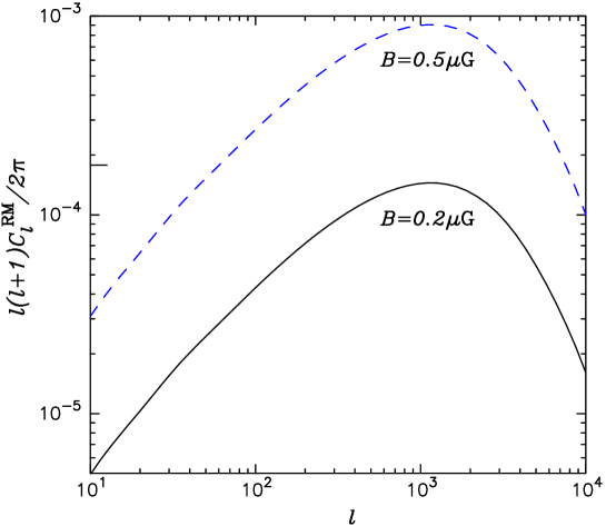
Figure 2: The angular power spectra of the rotation measure angle due the intracluster magnetic field calculated by equation (10) for the observed frequency of $10{\rm GHz}$ in the LCDM model ($\Omega_{m0}=0.3$, $\Omega_{\lambda 0}=0.7$, $h=0.7$, $\Omega_{b0}=0.05$, $\sigma_{8}=1$). We here considered two cases of the uniform magnetic fields $B_{0}$ of $0.2~{}\mu{\rm G}$ (solid line) and $0.5~{}\mu{\rm G}$ (dashed) strength across a cluster. Note that the power spectrum has the dependence on the magnetic field strength and the observed frequency as $\propto B_{0}^{2}\nu_{0}^{-4}$.

3 Secondary Effect of Faraday Rotation in a Cluster on CMB Polarization

In this section we develop a formalism for calculating the secondary Faraday rotation effect induced by magnetized intracluster hot plasma on the CMB polarization fields and their angular power spectra.

The properties of CMB polarization fields can be described in terms of the Stokes parameters $Q$ and $U$ (Kosowsky (1996); Kamionkowski, Kosowsky, & Stebbins 1997a ,b; Zaldarriaga, & Seljak (1997)). Let us consider quasi-monochromatic waves propagating in the z-direction, in which the electric and magnetic fields vibrate on the $x$-$y$ plane. We can then express the electric field $E$ in terms of the complex orthogonal unit vectors of circularly polarized waves as $\mbox{\boldmath$E$}=(E_{\rm R}e^{i\delta_{\rm R}}\mbox{\boldmath$\epsilon$}_{R}+E_{\rm L}e^{i\delta_{\rm L}}\mbox{\boldmath$\epsilon$}_{\rm L})e^{-i\omega t}$, where $\mbox{\boldmath$\epsilon$}_{\rm R,L}\equiv(\mbox{\boldmath$\epsilon$}_{x}\mp i\mbox{\boldmath$\epsilon$}_{y})/\sqrt{2}$ and $\mbox{\boldmath$\epsilon$}_{\rm R}$ and $\mbox{\boldmath$\epsilon$}_{\rm L}$ are the unit vectors of right-hand and left-hand polarized waves, respectively. Using those quantities, the Stokes parameters $Q$ and $U$ measured in the fixed $(x,y)$-coordinates can be expressed as

$$Q \equiv |\mbox{\boldmath$E$}\cdot\mbox{\boldmath$\epsilon$}_{x}|^{2}-|\mbox{\boldmath$E$}\cdot\mbox{\boldmath$\epsilon$}_{y}|^{2}=2E_{\rm R}E_{\rm L}\cos(\delta_{\rm R}-\delta_{\rm L}),$$

$$U \equiv 2{\rm Re}\left[(\mbox{\boldmath$E$}\cdot\mbox{\boldmath$\epsilon$}_{x})^{\ast}(\mbox{\boldmath$E$}\cdot\mbox{\boldmath$\epsilon$}_{y})\right]=2E_{\rm R}E_{\rm L}\sin(\delta_{\rm R}-\delta_{\rm L}).$$ (12)

If there is an intervening magnetic field in the ionized plasma between the last scattering surface and the present epoch, the right-hand and left-hand polarized waves travel with different phase velocities by the Faraday rotation effect. Therefore, from equation (12), we can derive the following equation to govern the time evolution of $Q$ and $U$ in the presence of the magnetized plasma;

$$\frac{dQ}{dt} =- U\frac{d(\delta_{\rm R}-\delta_{\rm L})}{dt}=-2\omega_{B}U,$$

$$\frac{dU}{dt} = 2\omega_{B}Q,$$ (13)

where $2\omega_{B}\equiv d(\delta_{R}-\delta_{\rm L})/dt$, $t$ is the cosmic time and we have ignored other effects associated with the Thomson scattering. Note that $\omega_{B}$ is also related to the rotation measure angle $\Delta\varphi$ defined by equation (1) as $\omega_{B}=d(\Delta\varphi)/dt$. Equation (13) clearly shows that the Faraday rotation causes the mixing between $Q$- and $U$-type polarizations. More importantly, even if the primary CMB anisotropies generate only the $Q$-type polarization in the statistical sense (Zaldarriaga, & Seljak (1997)), the Faraday rotation mixing induces the $U$-type polarization on the observed sky from the primary $Q$ mode.

Since we are interested in the secondary effect on the CMB polarizations, the solutions of equation (13) for $Q$ and $U$ along the line of sight with direction of $\theta$ can be approximately solved up to the first order of $\omega_{B}$ as

$$Q(t_{0},\mbox{\boldmath$\theta$}) \approx \tilde{Q}(t_{\ast},\mbox{\boldmath$\theta$})-2\tilde{U}(t_{\ast},\mbox{\boldmath$\theta$})\int^{t_{0}}_{t_{\ast}}\!\!dt\omega_{B}(t,\mbox{\boldmath$\theta$})$$

$$U(t_{0},\mbox{\boldmath$\theta$}) \approx \tilde{U}(t_{\ast},\mbox{\boldmath$\theta$})+2\tilde{Q}(t_{\ast},\mbox{\boldmath$\theta$})\int^{t_{0}}_{t_{\ast}}\!\!dt\omega_{B}(t,\mbox{\boldmath$\theta$}),$$ (14)

where $\tilde{U}$ and $\tilde{Q}$ denote the primary $U$- and $Q$-polarization fluctuations generated at the decoupling epoch ($z_{\ast}\approx 10^{3}$), respectively, and we have neglected other secondary polarization fields generated at low redshifts that have insignificant power compared to the primary signal on relevant angular scales for a realistic reionization history (e.g., Hu (2000)). The quantities $t_{\ast}$ and $t_{0}$ are the cosmic time at the decoupling and the present time, respectively. In what follows quantities with tilde symbol denote quantities at $t_{\ast}$.

The Stokes parameters $Q$ and $U$ depend on the choice of coordinates and are not invariant under the coordinate rotation. For this reason, it is useful to introduce the new bases of rotationally invariant polarization fields, called the parity-even electric mode ($E$) and the parity-odd magnetic mode ($B$) (Zaldarriaga, & Seljak (1997); Kamionkowski, Kosowsky, & Stebbins 1997a ,b; Hu, & White 1997a ,b). Any polarization pattern on the sky can be decomposed into these modes. Since the secondary effect due to clusters of galaxies on the CMB polarization is important only on small angular scales such as $\theta\lower 2.15277pt\hbox{$\;\buildrel<\over{\sim}\;$}1^{\circ}$, we can safely employ the small-angle approximation (Zaldarriaga, & Seljak (1998)). Based on these considerations, $Q$ and $U$ fields can be expressed using the two-dimensional Fourier transformation in terms of the electric and magnetic modes as

$$Q(\mbox{\boldmath$\theta$}) = \int\!\!\frac{d^{2}\mbox{\boldmath$l$}}{(2\pi)^{2}}\left[E_{\mbox{\boldmath$l$}}\cos 2\phi_{\mbox{\boldmath$l$}}-B_{\mbox{\boldmath$l$}}\sin 2\phi_{\mbox{\boldmath$l$}}\right]e^{i\mbox{\boldmath$l$}\cdot\mbox{\boldmath$\theta$}},$$

$$U(\mbox{\boldmath$\theta$}) = \int\!\!\frac{d^{2}\mbox{\boldmath$l$}}{(2\pi)^{2}}\left[E_{\mbox{\boldmath$l$}}\sin 2\phi_{\mbox{\boldmath$l$}}+B_{\mbox{\boldmath$l$}}\cos 2\phi_{\mbox{\boldmath$l$}}\right]e^{i\mbox{\boldmath$l$}\cdot\mbox{\boldmath$\theta$}},$$ (15)

where $\phi_{\mbox{\boldmath$l$}}$ is defined by $l_{x}+il_{y}=l\exp(i\phi_{\mbox{\boldmath$l$}})$, and $E_{\mbox{\boldmath$l$}}$ and $B_{\mbox{\boldmath$l$}}$ are the two-dimensional Fourier coefficients for the $E$- and $B$-modes, respectively. The Fourier components $\tilde{E}_{\mbox{\boldmath$l$}}$ and $\tilde{B}_{\mbox{\boldmath$l$}}$ for the primary CMB polarization fields satisfy

$$\left\langle{\tilde{E}_{\mbox{\boldmath$l$}}\tilde{E}^{\ast}_{\mbox{\boldmath$l$}^{\prime}}}\right\rangle=(2\pi)^{2}C_{\tilde{E}l}\delta^{2}(\mbox{\boldmath$l$}-\mbox{\boldmath$l$}^{\prime}),$$

$$\left\langle{\tilde{B}_{\mbox{\boldmath$l$}}\tilde{B}^{\ast}_{\mbox{\boldmath$l$}^{\prime}}}\right\rangle=(2\pi)^{2}C_{\tilde{B}l}\delta^{2}(\mbox{\boldmath$l$}-\mbox{\boldmath$l$}^{\prime}),$$ (16)

where $C_{\tilde{E}l}$ and $C_{\tilde{B}l}$ are the angular power spectra of primary $E$- and $B$-modes, respectively. The primary $B$-mode polarization is generated by the quadrupole temperature anisotropies associated with the tensor (gravitational wave) and vector perturbations. If we assume the standard inflation-motivated model with a spectral index of $n_{\rm s}=1$ for the scalar perturbations, the tensor and vector perturbations are sufficiently smaller than the scalar perturbations. In the following discussion we ignore the primary $B$-mode power spectrum for simplicity; $C_{\tilde{B}l}=0$.

From equation (14) the two-point correlation functions of $Q$ and $U$ fields including the Faraday rotation mixing effect can be computed as

$$C_{Q}(\theta) \equiv \left\langle{Q(0)Q(\mbox{\boldmath$\theta$})}\right\rangle\approx C_{\tilde{Q}}(\theta)+4C_{\tilde{U}}(\theta)C^{{\rm RM}}(\theta),$$

$$C_{U}(\theta) \equiv \left\langle{U(0)U(\mbox{\boldmath$\theta$})}\right\rangle\approx C_{\tilde{U}}(\theta)+4C_{\tilde{Q}}(\theta)C^{{\rm RM}}(\theta),$$ (17)

with

$$C_{\tilde{Q}}(\theta) = \int\!\!\frac{ldl}{2\pi}\frac{C_{\tilde{E}l}}{2}(J_{0}(l\theta)+J_{4}(l\theta)),$$

$$C_{\tilde{U}}(\theta) = \int\!\!\frac{ldl}{2\pi}\frac{C_{\tilde{E}l}}{2}(J_{0}(l\theta)-J_{4}(l\theta)),$$ (18)

where we have employed a reasonable assumption that the primary fields ($\tilde{Q}$ and $\tilde{U}$) on the last scattering surface and the rotation measure field $\omega_{B}$ induced by low-$z$ clusters are statistically uncorrelated. Note that $C^{{\rm RM}}(\theta)$ is the two-point correlation function of the rotation measure angle and can be expressed in terms of the angular power spectrum of the rotation measure as

$$C^{\rm RM}(\theta)\equiv\left\langle{\int\!\!dt\omega_{B}(t,0)\int\!\!dt^{\prime}\omega_{B}(t^{\prime},\mbox{\boldmath$\theta$})}\right\rangle=\int\!\!\frac{ldl}{2\pi}C^{\rm RM(P)}_{l}J_{0}(l\theta),$$ (19)

where $C^{\rm RM(P)}_{l}$ is given by equation (10).

We are now in the position to derive the angular power spectra of $E$ and $B$ modes in the observed CMB sky. Following the method developed by Zaldarriaga, & Seljak (1998), $C_{El}$ and $C_{Bl}$ can be expressed as

$$C_{El} = \pi\int^{\pi}_{0}\!\theta d\theta\left[(C_{Q}(\theta)+C_{U}(\theta))J_{0}(l\theta)+(C_{Q}(\theta)-C_{U}(\theta))J_{4}(l\theta)\right],$$

$$C_{Bl} = \pi\int^{\pi}_{0}\!\theta d\theta\left[(C_{Q}(\theta)+C_{U}(\theta))J_{0}(l\theta)-(C_{Q}(\theta)-C_{U}(\theta))J_{4}(l\theta)\right].$$ (20)

Therefore, from equation (18) we have

$$C_{El} = C_{\tilde{E}l}+\int\!\!l^{\prime}dl^{\prime}W^{E}_{ll^{\prime}}C_{\tilde{E}l^{\prime}}$$

$$C_{Bl} = \int\!\!l^{\prime}dl^{\prime}W^{B}_{ll^{\prime}}C_{\tilde{E}l^{\prime}},$$ (21)

where $W_{Ell^{\prime}}$ and $W_{Bll^{\prime}}$ are the window functions defined by

$$W^{E}_{ll^{\prime}} \equiv 2\int_{0}^{\pi}\!\theta d\theta\left[J_{0}(l\theta)J_{0}(l^{\prime}\theta)-J_{4}(l\theta)J_{4}(l^{\prime}\theta)\right]C^{\rm RM}(\theta),$$

$$W^{B}_{ll^{\prime}} \equiv 2\int_{0}^{\pi}\!\theta d\theta\left[J_{0}(l\theta)J_{0}(l^{\prime}\theta)+J_{4}(l\theta)J_{4}(l^{\prime}\theta)\right]C^{\rm RM}(\theta).$$ (22)

Equations (21) clearly show that the Faraday rotation mixing generates the non-vanishing angular power spectrum of the $B$-mode polarization from the primary $E$-mode.

4 Results and Estimations of the Detectability

Throughout this paper, we employ the $\Lambda$CDM model with $\Omega_{m0}=0.3$, $\Omega_{\lambda 0}=0.7$, $\Omega_{b0}=0.05$, $h=0.7$ and $\sigma_{8}=1.0$ as supported from observations of the CMB anisotropies and the large-scale structure. As for the power spectrum of dark matter used in the calculation of the Press-Schechter mass function, we adopted the Harrison-Zel’dovich spectrum and the BBKS transfer function (Bardeen et al. (1986)) with the shape parameter from Sugiyama (1995).

Figure 3 shows the window functions of $B$- and $E$-modes per logarithmic interval in $l$, $l^{2}W^{B}_{ll^{\prime}}$ and $l^{2}W^{E}_{ll^{\prime}}$, for a given mode $l^{\prime}=2000$ as derived by equation (22). We consider the magnetic field strength $B_{0}=0.2~{}\mu{\rm G}$ and the observed frequency $10~{}{\rm GHz}$ in the $\Lambda$CDM model. One can see that the window functions for the mixing between $E$ and $B$ modes are well localized in $l$ space.

In Figure 4 we show the angular power spectra of $E$- and $B$-mode polarizations on the observed sky including the Faraday rotation mixing effect due to clusters for the observed frequency of $10{\rm GHz}$. The dot-dashed line shows the $B$-mode spectrum for $B_{0}=0.5\mu{\rm G}$ that corresponds to the value estimated from the observational data for a model of uniform intracluster magnetic field (Clarke et al. 2001), while the dotted line shows the result of $B_{0}=0.2\mu{\rm G}$. For comparison, the $E$-mode power spectra with and without the secondary effect of $B_{0}=0.2\mu{\rm G}$ are also shown by solid and dashed lines, respectively. One can readily see that the generated $B$-mode power spectrum has a peak with magnitude of $\sim 0.1~{}\mu{K}(B_{0}/0.1~{}\mu{G})(\nu_{0}/10~{}{\rm GHz})^{-2}$ at $l\approx 1000$. On smaller scales of $l\lower 2.15277pt\hbox{$\;\buildrel>\over{\sim}\;$}6000$, the spectra of $E$ and $B$ modes coincide, and this is similar as the secondary effects caused by the peculiar velocity field of the ionized medium in the reionized universe (Hu (2000); Liu et al. (2001)). These results imply that, if the uniform magnetic field has a strength of $\sim 0.5~{}\mu{\rm G}$ and we can observe at lower frequencies such as $\nu_{0}\lower 2.15277pt\hbox{$\;\buildrel<\over{\sim}\;$}5~{}{\rm GHz}$, the magnitude of $B$-mode could be comparable with the primary polarization amplitude of $\sim\mu{\rm K}$.

The detectability of the induced $B$ mode polarization by the sensitive satellite mission Planck can be estimated following the method developed by Zaldarriaga & Seljak (1998). The relative error on the overall amplitude of the induced $B$ component $\beta$ can be estimated as

$$\frac{\Delta\beta}{\beta}=\sqrt{\frac{2}{f_{\rm sky}\sum_{l}(2l+1)/(1+w^{-1}e^{l^{2}\theta_{s}^{2}}/C_{\tilde{B}l})^{2}}},$$ (23)

where $f_{\rm sky}$ is the fraction of observed sky and we here fix $f_{\rm sky}=0.8$. As for the detector noise and the beam width, we assume $w^{-1}=4.72\times 10^{-16}$ and $\theta_{\rm s}=\theta_{\rm fwhm}/\sqrt{8\ln 2}=3.71\times 10^{-3}$ for the $30$GHz channel on Planck, where $\theta_{\rm fwhm}$ is the full-width at half-maximum angle. Note that the $30$GHz channel we here consider is the lowest frequency channel on Planck. From the dependence $\lambda_{0}^{2}$ of the rotation measure, the magnitude of the $B$-mode angular power spectrum at $30$GHz becomes smaller by $\sim 10^{-2}$ than the results estimated in Figure 4. Accordingly, for the magnetic field of $B_{0}=0.2~{}\mu{\rm G}$, we have $\beta/\Delta\beta\approx 0.14$. This means that this effect cannot be detected by the Planck mission for $B_{0}=0.2\mu{\rm G}$. Conversely, to get $\beta/\Delta\beta\approx 1$ at the $30$GHz channel, the uniform magnetic field component must have $\sim 1.5~{}\mu{\rm G}$ strength, and this seems an unrealistic value. However, we stress that even a null detection of this effect can set a new constraint on the magnetic field strength. It is also worth noting that this signal would be detected more effectively by a ground based experiments at lower frequency bands such as $\lower 2.15277pt\hbox{$\;\buildrel<\over{\sim}\;$}10~{}{\rm GHz}$ observing a small patch of the sky for a sufficiently long integration time to reduce the noise per pixel.

Figure 3: This figure shows the weighted window functions $l^{2}W^{B}_{ll^{\prime}}$ and $l^{2}W^{E}_{ll^{\prime}}$ defined by equation (22) as a function of $l$ for a given mode $l^{\prime}=2000$. We here present their power per logarithmic interval in $l$. We used the model of the magnetic field strength $0.2~{}\mu{\rm G}$ and the observed frequency $10~{}{\rm GHz}$.

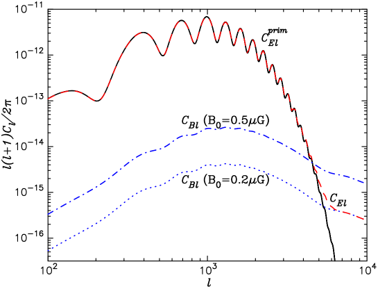
Figure 4: The angular power spectra of $E$- and $B$-mode polarizations. The dashed and dotted lines show the $E$- and $B$-mode spectra including the Faraday mixing effect due to clusters at the observed frequency of $10~{}{\rm GHz}$ for the magnetic field model of $B_{0}=0.2~{}\mu{\rm G}$, respectively, while the dot-dashed line shows the $B$-mode spectrum for the case of $B_{0}=0.5~{}\mu{\rm G}$ that corresponds to the value estimated by Clarke et al. (2001) for a model of the uniform magnetic field. For comparison, the solid line shows the primary $E$-mode power spectrum in the $\Lambda$CDM model.

5 Discussions and Conclusions

In this paper, we have investigated the secondary effect on the CMB polarization fields induced by the Faraday rotation effect of the magnetic field in an intracluster hot plasma at a low redshift. To illustrate the impact of this effect in the simplest way, we employed the simple model that the magnetic field has a uniform field strength such as $0.2~{}\mu{\rm G}$ across a cluster universally when the cluster formed, which is consistent with observations of the rotation measures in clusters (Clarke et al. 2001). As shown in Figure 1, our model can roughly reproduce the observed scatter of the rotation measures as a function of the distance from the cluster center (Kim et al. 1991; Clarke et al. 2001). In this sense, since the Faraday rotation effect on the angular power spectra of CMB polarizations comes from the second moments of the rotation measure angle (see equation (21)), it is likely that our model can at least estimate a correct magnitude of the effect, even though detailed shapes of those spectra could be different for a realistic intracluster magnetic field as discussed below. We showed that the parity-odd $B$-mode angular power spectrum is generated on the observed sky by the Faraday rotation mixing effect as a new qualitative feature, when if the primary CMB anisotropies includes the parity-even $E$-mode only such as predicted by the standard inflation-motivated scenarios with pure primordial scalar perturbations. We estimated that the generated $B$-mode power spectrum has a peak with amplitude of $\sqrt{l^{2}C_{lB}/2\pi}\sim 0.1~{}\mu{\rm K}(B_{0}/0.1~{}\mu{\rm G})(\nu_{0}/10~{}{\rm GHz})^{-2}$ at $l\approx 1000$ under the plausible scenario of the cluster formation in the currently favored $\Lambda$CDM model. It was also shown that the lowest frequency $30{\rm GHz}$ channel of Planck can be used to set an upper limit of $B_{0}\lower 2.15277pt\hbox{$\;\buildrel<\over{\sim}\;$}1.5\mu{\rm G}$ for a uniform component of the intracluster magnetic field. Detection or even null detection of the predicted $B$-type polarization will therefore be a new empirical tool to provide a calibration of an uncertain magnetic field in a cluster, combined with measurements of the gas distribution from the X-ray or SZ datasince.

It is known that there are other secondary sources on the CMB polarization fields caused in the low redshift universe, and these nonlinear effects generally induce the $B$-type polarization pattern from the coupling with the primary $E$-mode. The main source is the gravitational lensing effect of the large-scale structure, leading to the $B$-type polarization that has a peak of $\sim 0.3~{}\mu{\rm K}$ at $l\approx 1000$ and then a power of $\lower 2.15277pt\hbox{$\;\buildrel<\over{\sim}\;$}0.01~{}\mu{\rm K}$ at $l\lower 2.15277pt\hbox{$\;\buildrel>\over{\sim}\;$}5000$ for the simliar $\Lambda$CDM model as considered in this paper (Zaldarriaga, & Seljak (1998)). One of authors (N.S.) has quantitatvely shown that the secondary effect due to the peculiar motion of ionized medium in the large-scale structure also generates the $B$-mode polarization with $\sim 0.01~{}\mu{K}$ at $100\lower 2.15277pt\hbox{$\;\buildrel<\over{\sim}\;$}l\lower 2.15277pt\hbox{$\;\buildrel<\over{\sim}\;$}10^{4}$ for a realistic patchy reionization model of the universe (Liu et al. (2001)). From these results, if the uniform magnetic field has a larger strength of $B\sim 0.5~{}\mu{\rm G}$ as a common feature of clusters and we observe at lower frequencies such as $\nu_{0}\lower 2.15277pt\hbox{$\;\buildrel<\over{\sim}\;$}5~{}{\rm GHz}$, the generated $B$-mode amplitude due to the Faraday rotation effect would be comparable with the primary polarization amplitude and larger than the other secondary signals at $l\lower 2.15277pt\hbox{$\;\buildrel>\over{\sim}\;$}1000$, although observations at such low frequencies would suffer from large foreground contamination of the syncrhrotron radiation from our galaxy (Tegmark et al. (2000)). Even if the uniform magnetic field is not as strong as $0.5~{}\mu{\rm G}$, the sensitive multi low-frequency measurements will allow one to separate this signal from primary and those other secondary signals in principle thanks to the frequency dependence of $\propto\nu_{0}^{-4}$ on $C_{Bl}$, which is analogous to measurements of secondary temperature fluctuations by the SZ effect.

There are possible contributions to affect our results that we have ignored in this paper. The intracluster tangled magnetic fields, as implied by the rotation measures of some sources inside the Coma cluster (Kim et al. (1990)), would provide contributions to our results in addition to the contribution due to the uniform field. However, the coherent scale of tangled fields in a cluster is still unknown. The recent complete measurements of the rotation measures (Clarke et al. 2001) imply the $1-10~{}\mu{\rm G}$ strength of the tangled field under the assumption of the coherent scale of $10-100~{}{\rm kpc}$. It is also known that the strong radio halos embedded within a (cooling flow) cluster are pervaded by stronger magnetic fields on smaller scales such as $\sim 50~{}{\mu G}$ for Hydra A (Taylor, & Perley (1993); Taylor et al. (2001)). Although the simplest tangled-cell model with a constant coherence length $l$ has often been considered in the literature, the possible important mechanism to affect our results is the deporlarization effect (Tribble (1991)), leading to the cancellations to some extent between the Faraday rotations in independent cells with random orientations of the magnetic fields within a cluster. The finite beam size will also lead to the artificial cancellations between the Faraday rotations of cells covered within one beam. From these considerations, the depolarization effect may lead to an intuitive result that a feature of the $B$-mode spectrum can be sensitive to the characteristic angular scale, $l_{c}$, originating from the coherent length. This investigation is now in progress, and will be presented elsewhere (Ohno et al. 2001). Recently, it has been suggested that outflow or jet acitivities of quasars or black holes leave behind an expanding magnetized bubble in the itergalactic medium (IGM) resulting in the possibility that the IGM is filled by magnetic fields to some extent (Furlanetto, & Loeb (2001); Kronberg et al. (2001)). Even thgouh the IGM field has a smaller strength than $\sim 10^{-9}{\rm~{}G}$ on ${\rm Mpc}$ scales, a large volume coverage of the ionized plasma might lead to non-negligible contribution connected to the reionization history of the universe.

Finally, we comment on implications of our results to the nonthermal processes in a cluster. The observations of diffuse synchrotron halos and nonthermal hard X-ray emission have implied the existence of nonthermal relativistic electrons in a cluster (e.g., Rephaeli, Gruber, & Blanco (1999)). These electrons are produced by the shock acceleration in an intracluster medium, and it will allow us to derive additional information on the physical conditions of the intracluster medium environment, which cannot be obtained from the thermal plasma emission only. The intracluster magnetic field should then play an important role to these nonthermal processes. In particular, it is being recognized that the nonthermal process can be a unique probe of measuring the dynamically forming clusters before thermalization of the intracluster gas. Recently, Waxman & Loeb (2000) pointed out that the synchrotron radiation from those forming clusters could be foreground sources of the CMB temperature fluctuations at low frequency observations such as $10{\rm~{}GHz}$. Those clusters could also produce the high energy gamma ray emission through the inverse Compton scattering of CMB photons by relativistic electrons and thus be identified as gamma ray clusters by the future sensitive telescope GLAST, which are difficult to detect by X-ray or optical surveys because of their extended angular size of about $\sim 1^{\circ}$ (Totani, & Kitayama (2000)). Based on these ideas, it will be very interesting to investigate cross-correlations between the synchrotron radiation or the gamma ray sources and the Faraday rotation signal in CMB polarization map. This investigation is expected to provide complementary constraints on the nonthermal physical processes in the forming clusters.

References

- Adams et al. (1996) Adams, J., Danielsson, U. H., Grasso, D., & Rubinstein, H., Phys. Lett. B, 388, 253
- Atrio-Barandela, & Mücket (1999) Atrio-Barandela, F., & Mücket, J. P., 1999, ApJ, 515, 465
- Bagchi, Pislar, & Neto (1998) Bagchi, J., Pislar, V., & Neto, G. B. L. 1998, MNRAS, 296, L23
- Bardeen et al. (1986) Bardeen, J. M., Bond., J. R., Kaiser, N., & Szalay, A. S. 1986, ApJ, 304, 15
- Bower (1997) Bower, R. G., 1997, MNRAS, 288, 355
- Bond, & Efstathiou (1987) Bond, J. R., & Efstathiou, G. P. 1987, MNRAS, 226, 655
- Bryan, & Norman (1998) Bryan, G. L., & Norman, M.,L. 1998, ApJ, 495, 80
- Carilli, & Taylor (2001) Carilli, C. L., & Taylor, G. B. 2001, astro-ph/0110655
- Clarke, Krongerb, & Böhringer (2001) Clarke, T. E., Krongerg, P. P., & Böhringer, H. 2001, ApJ, 547, L111
- Cole, & Kaiser (1988) Cole, S., & Kaiser, N. 1988, MNRAS, 233, 637
- Cooray (2000) Cooray, A. 2000, Phys. Rev. D, 62, 103506
- Dolag, Bartelmann, & Lesch (1999) Dolag, K., Bartelmann, M., & Lesch, H. 1999, A&A, 348, 351
- Eke, Navarro, & Frenk (1998) Eke, V. R., Navarro, J. F., & Frenk, C. S. 1998, ApJ, 503, 569
- Evrard, & Henry (1991) Evrard, A. E., & Henry, J. P. 1991, ApJ, 383, 95
- Feretti et al. (1995) Feretti, L., Dallacasa, D., Giovannini, G., & Tagliani, A. 1995, A&A, 302, 680
- Furlanetto, & Loeb (2001) Furlanetto, S. R., & Loeb, A. 2001, astro-ph/0102076
- Fusco-Femiano et al. (1999) Fusco-Femiano, R. et al. 1999, ApJ, 513, L21
- Grasso, & Rubinstein (2000) Grasso, D., & Rubinstein, H. R. 2000, to appear in Phys. Rep., astro-ph/0009061
- Harari, Hayward, & Zaldarriaga (1997) Harari, D. D., Hayward, J. D., & Zaldarriaga, M. 1997, Phys. Rev. D, 55, 1841
- Hu (2000) Hu, W. 2000, ApJ, 529, 12
- (21) Hu, W., & White, M. 1997, Phys. Rev. D, 56, 596
- (22) Hu, W., & White, M. 1997, NewA, 2, 232
- Hu, & Sugiyama (1995) Hu, W., & Sugiyama, N. 1995, ApJ, 444, 489
- Jones, & Forman (1984) Jones, C. & Forman, W. 1984, ApJ, 276, 38
- Kaiser (1986) Kaiser, N. 1986, MNRAS, 222, 323
- Kaiser (1991) Kaiser, N. 1991, ApJ, 383, 104
- (27) Kamionkowski, M., Kosowsky, A., & Stebbins, A. 1997, Phys. Rev. Lett., 78, 2058
- (28) Kamionkowski, M., Kosowsky, A., & Stebbins, A. 1997, Phys. Rev. D, 55, 7368
- Kim et al. (1990) Kim, K.-T., Kronberg, P. P., Dewdney, P. E., Landecker, T. L. 1990, ApJ, 355, 29
- Kim, Tribble, & Kronberg (1991) Kim, K.-T., Tribble, P. C., & Kronberg, P. P. 1991, ApJ, 379, 80
- Komatsu, & Kitayama (1999) Komatsu, E., & Kitayama, T. 1999, ApJ, 526, L1
- Kosowsky (1996) Kosowsky, A. 1996, Ann. Phys., 246, 49
- Kosowsky, & Loeb (1996) Kosowsky, A., & Loeb, A. 1996, ApJ, 469, 1
- Kronberg (1994) Kronberg, P. P. 1994, Rep.Prog.Phys., 57, 325
- Kronberg, Lesch, & Hopp (1999) Kronberg, P. P., Lesch, H., & Hopp, U. 1999, ApJ, 511, 56
- Kronberg et al. (2001) Kronberg, P. P., Dufton, Q. W., Li, H., & Colgate, S. A. 2001, astro-ph/0106281
- Lesch, & Chiba (1997) Lesch, H., & Chiba, M. 1997, Fundam. Cosmic Phys., 18, 273
- Liu et al. (2001) Liu, G.-C., Sugiyama, N., Benson, A. J., Lacey, C. G., & Nusser, A., submitted to ApJ, astro-ph/0101316
- Loeb, & Mao (1994) Loeb, A., & Mao, S. 1994, ApJ, 435, L109
- Loeb, & Waxman (2000) Loeb, A., & Waxman, E. 2000, Nature, 405, 156
- Mack, Kahniashvili, & Kosowsky (2001) Mack, A., Kahniashvili, T., & Kosowsky, A. 2001, astro-ph/105504
- Makino, Sasaki & Suto (1998) Makino, N., Sasaki, S., & Suto, Y. 1998, ApJ, 497, 555
- Navarro, Frenk, & White (1997) Navarro, Frenk, & White 1997, ApJ, 490, 493
- Netterfield et al. (2001) Netterfield et al. 2001, astro-ph/0104460
- Ohno et al. (2001) Ohno, H., Takada, M., Dolag, K., Bartelmann, M., & Sugiyama, N. 2001, in preparation
- Parker (1979) Parker, E. N. 1979, Cosmical Magnetic Fields (Oxford: Clarendon)
- Peebles (1980) Peebles, P. J. E. 1980, The Large Scale Structure of the Universe (Princeton; Princeton Univ. Press)
- Press, & Schechter (1974) Press, W. H., & Schechter, P. 1974, ApJ, 187, 425
- Rees (1987) Rees, M. 1987, QJRAS, 28, 197
- Rephaeli, Gruber, & Blanco (1999) Rephaeli, Y., Gruber, D. E., & Blanco, P. 1999 ApJ, 511, L21
- Rybicki, & Lightman (1979) Rybicki, G. B., & Lightman, A. P. 1979, Radiative Processes in Astrophysics (New York: John Wiley & Sons)
- Scannapieco, & Ferreira (1997) Scannapieco, E. S., & Ferreira, P. G., 1997, Phys. Rev. D, 56, R7493
- Seshadri, & Subramanian (2001) Seshadri, T. R., & Subramanian, K., 2001, Phys. Rev. Lett. in press, astro-ph/0012056
- Silk (1968) Silk, J. 1968, ApJ, 151, 459
- Sugiyama (1995) Sugiyama, N. 1995, ApJS, 100, 281
- Taylor, & Perley (1993) Taylor, G. B., Perley, R. A. 1993, ApJ, 416, 554
- Taylor et al. (2001) Taylor, G. B., Govoni, F., Allen, S. A., & Fabian, A. C. 2001, astro-ph/0204223
- Tegmark et al. (2000) Tegmark, M., Eisenstein, D. J., Hu, W., & de Oliveira-Costa, A. O. 2000, ApJ, 530, 133
- Totani, & Kitayama (2000) Totani, T., & Kitayama, T. 2000, 545, 572
- Tribble (1991) Tribble, P. C. 1991, MNRAS, 250, 726
- Vallée, MacLeod, & Broten (1986) Vallée, J. P., MacLeod, J. M., & Broten, N. W. 1986, A&A, 156, 386
- Vikhlinin, Markevitch, & Murray (2001) Vikhlinin, A., Markevitch, M., & Murray, S. S. 2001, ApJ, 549, L47
- Waxman, & Loeb (2000) Waxman, E., & Loeb, A. 2000, ApJ, 545, L11
- Welter, Perry, & Kronberg (1984) Welter, G. L., Perry, J. J., & Kronberg, P. P. 1984, ApJ, 279, 19
- White et al. (1993) White, S. D. M., Navarro, J. F., Evrard, A. E., & Frenk, C. S. 1993, Nature, 366, 429
- Wolfe, Lanzetta, & Oren (1992) Wolfe, A. M., Lanzetta, K., & Oren, A. L. 1992, ApJ, 388, 17
- Zaldarriaga, & Seljak (1997) Zaldarriaga, M., & Seljak, U. 1997, Phys. Rev. D, 55, 1830
- Zaldarriaga, & Seljak (1998) Zaldarriaga, M., & Seljak, U. 1998, Phys. Rev. D, 58, 023003
- Zel’dovich, Ruzmaikin, & Sokoloff (1983) Zel’dovich, Ya. B., Ruzmaikin, A. A., & Sokoloff, D. D. 1983, Magnetic Fields in Astrophysics, The Fluid Mechanics of Astrophysics and Geophysics, Vol. 3 (New York: Gordon & Breach)