Shocked molecular gas towards the SNR G359.1–0.5 and the Snake

Abstract

We have found a bar of shocked molecular hydrogen (H₂) towards the OH(1720 MHz) maser located at the projected intersection of supernova remnant (SNR) G359.1–0.5 and the nonthermal radio filament, known as the Snake. The H₂ bar is well aligned with the SNR shell and almost perpendicular to the Snake. The OH(1720 MHz) maser is located inside the sharp western edge of the H₂ emission, which is consistent with the scenario in which the SNR drives a shock into a molecular cloud at that location. The spectral–line profiles of ¹²CO, HCO⁺ and CS towards the maser show broad–line absorption, which is absent in the ¹³CO spectra and most probably originates from the pre–shock gas. A density gradient is present across the region and is consistent with the passage of the SNR shock while the H₂ filament is located at the boundary between the pre–shocked and post-shock regions.

1 Introduction

OH(1720 MHz) maser emission detected towards supernova remnants (SNRs) has been attributed to shock waves driven into adjacent molecular clouds (Frail, Goss & Slysh, 1994). The production of this maser emission, without the simultaneous production of maser emission in the other three ground state OH transitions at 1612, 1665 and 1667 MHz, requires specific conditions (gas density $n_{\scriptscriptstyle\rm H_{2}}$$\sim$$10^{5}$ cm^-3, gas temperature $T_{kin}$$\sim$50 – 125 K, OH column density $N_{\rm OH}\sim$ $10^{15}$ – $10^{16}$ cm^-2) which can be attained in the cooling gas behind a non-dissociative shock wave (Lockett, Gauthier & Elitzur, 1999; Wardle, 1999). Surveys by Frail et al. (1996), Green et al. (1997) and Koralesky et al. (1998) have found that about 10 per cent of $\sim$180 observed Galactic SNRs are associated with OH(1720 MHz) masers. The detection fraction increases to 30 per cent for objects in the Galactic Centre region (Yusef-Zadeh et al., 1996a).

Perhaps the most striking result of the survey towards the Galactic Centre region is the detection of OH masers along the radio–continuum shell of the SNR G359.1–0.5 (Yusef-Zadeh et al., 1995, 1996b). The brightest of the masers (maser A from Yusef-Zadeh et al. 1995) occurs where a nonthermal filament known as ‘the Snake’ appears to cross the western edge of the SNR shell. The filament differs from other Galactic Centre nonthermal filaments in showing a number of kinks along its 20 arcmin extent (Gray et al., 1995), and its origin is not well established (Nicholls & Le Strange, 1995; Benford, 1997; Uchida et al., 1996). The latest model by Bicknell & Li (2001) proposes that the Snake is a magnetic flux tube anchored in dense rotating material. It has been suggested that the Snake is interacting with the shell of G359.1–0.5 because both objects show change in brightness at the apparent crossing point (Uchida, Morris & Yusef-Zadeh, 1992; Gray et al., 1995). This could, however, be an artifact due to superposition of disparate components along the line of sight. Nevertheless, the presence of an OH(1720 MHz) maser – a signature of SNR/molecular cloud interaction – at this location is quite intriguing. In order to investigate the proposed interaction between the Snake and the SNR, and to characterise the ambient molecular gas in the region, we observed molecular hydrogen (H₂) and a number of other molecular species, particularly searching for signatures of shocked gas. The observations are discussed in section 2, the results are presented in section 3 and discussed in section 4. The conclusions are presented in section 5.

2 Observations

2.1 UNSWIRF observations

The observations towards maser A ($\rm{RA}(1950)=17^{\rm{h}}~{}41^{\rm{m}}~{}46\aas@@fstack{s}042$, $\rm{Dec.}~{}(1950)=-29\degr~{}49\arcmin~{}51\aas@@fstack{\prime\prime}03$) were carried out in June 1998 with UNSWIRF on the Anglo–Australian Telescope (AAT). Two data sets comprising five and six Fabry–Perot frames, each spaced by 40 km s^-1, were taken in the 2.12 $\micron$ H₂ 1–0 S(1) transition. An additional frame was taken at a setting of $-$400 km s^-1 to enable subsequent continuum subtraction. The integration time was 120 seconds per frame. A resulting image has diameter of 100 arcsec and a pixel size of 0.77 arcsec. The velocity resolution was $\sim$ 75 km s^-1  FWHM. All the data were reduced using modified routines in the iraf software package as described in Ryder et al. (1998). Intensity calibration was performed using the standard star BS 5699. A velocity cube was constructed by averaging the frames at the same Fabry–Perot setting from two data sets, which was then fitted with the instrumental Lorentzian profile to determine the line flux (to within 30 per cent) and central velocity (to within 20 km s^-1) for the H₂ emission across the field. We note that these data do not provide a true velocity–spatial cube of the emission, as the instrument does not have the velocity resolution to provide an accurate line velocity at each position. Rather, the line velocity is the central velocity at each position. Changes in line center velocity can, however, be determined. To confirm the detection, the observations were repeated in June 1999 for the 1–0 S(1) line and additional observations were obtained in the 2.25 $\micron$ H₂ 2–1 S(1) line. On this occasion five Fabry–Perot frames were used for both transitions, with an integration time of 180 seconds per frame. To establish the coordinate scale for the UNSWIRF images, we used the positions of stellar sources in the K-band continuum image listed in the Two Micron All Sky Survey (2MASS) point source catalogue (Cutri, 1997) (which has an accuracy of $\approx 0\aas@@fstack{\prime\prime}1$).

2.2 SEST observations

A millimetre–line survey towards maser A was carried out with the 15–m SEST at La Silla, Chile during June 2000. Position–switching was used with a reference position at $\rm{RA}(1950)=17^{\rm{h}}~{}45^{\rm{m}}~{}00^{s}$, $\rm{Dec.}~{}(1950)=-31\degr~{}00\arcmin~{}00\arcsec$. For periodic pointing calibration and focusing the 3-mm SiO maser of AH Sco was observed. The main–beam brightness temperature ($T_{mb}$) scale of the spectra was calibrated on–line using a black–body calibration source at ambient temperature, and later corrected for the telescope main–beam efficiency (0.74, 0.70, 0.67 and 0.45 at 85 – 100 GHz, 100 – 115 GHz, 130 – 150 GHz and 220 – 265 GHz respectively). Simultaneous observation of transitions in two different bands was available using dual SIS receivers at 3 and 2 mm, or 3 and 1.3 mm.

For spectral–line observing we used an acousto–optical spectrometer split into two 43–MHz bands, each with 1000 channels, providing velocity coverages ranging from 60 to 100 km s^-1 and velocity resolution ranging from 0.06 to 0.14 km s^-1  across the total wavelength range. A low–resolution spectrometer with resolution of $\sim$1–2 km s^-1 was also used simultaneously to determine the spectral baselines in the case of broad–line emission. The final data were smoothed over three channels. The observed transitions, frequencies and antenna beam sizes (FWHM) are listed in Table 1. For the ¹²CO, ¹³CO and CS transitions we obtained maps with approximately half–beam and one–beam sampling intervals at lower and higher transitions respectively. The final images covered the $2\times 2$ arcmin² region around maser A that coincides with the UNSWIRF field of view. The integration time was 30 seconds for CO isotopomers and 90 seconds for CS transitions. A set of spectra on–source and at offsets of 20 arcsec in RA and Dec. was obtained for each of the other molecular transitions listed in Table 1, with integration times of 180 seconds at each position.

Table 1: The first column lists observed molecular species, the next three columns list the SEST observational parameters and the last column gives observed main–beam brightness temperature ($T_{mb}$) and rms noise towards the maser A.

Molecule	Transition	Frequency	Beam Size	$T_{mb}$
		(GHz)	(arcsec)	(K)
13CO	2–1	220.399	23	0.78$\pm$0.21
	1–0	110.201	45	1.20$\pm$0.26
12CO	2–1	230.538	23	16.00$\pm$0.20
	1–0	115.271	45	10.30$\pm$0.50
CS	3–2	146.969	34	0.42$\pm$0.12
	2–1	97.981	52	0.54$\pm$0.14
HCO+	1–0	89.188	54	0.48$\pm$0.08
C18O	2–1	219.560	23	$<$ 0.16
	1–0	109.782	45	$<$ 0.12
HCN	1–0	88.632	55	$<$0.17
H2CO	3(2,2)–2(2,1)	218.475	24	$<$ 0.13
	3(0,3)–2(0,2)	218.222	24	$<$ 0.15
SiO	5–4	217.106	24	$<$ 0.14
	2–1	86.848	57	$<$0.17

The first part of the table lists results from Gaussian fit of the two ¹³CO transitions, whose line profiles peak at $-13$ km s^-1 and have line widths of $\sim$15 – 20 km s^-1. The second part of the table lists the parameters of ¹²CO, CS and HCO⁺ transitions. Their line profiles suffer broad–line absorption and Gaussian fitting was not possible. We therefore list only the maximum $T_{mb}$ of their line profiles, which occur at $-5$ km s^-1. The third part of the table lists the non–detections. Upper limits are 2$\sigma$ values.

3 Results and analysis

3.1 H₂ emission

Fig. 1 shows contours of velocity–integrated 2.12 $\micron$ H₂ 1–0 S(1) line emission superimposed on a greyscale image of the 2MASS K-band. Some small–scale structure apparent in the H₂ distribution are residuals from subtracting the stellar continuum. A bar of H₂ emission, 1.5 arcmin in length and 15 arcsec in width, extends from the north–east to the south–west. We note, however, that there is weak extensive diffuse emission across the observed region, which was not included in fitting procedure because low S/N. The lowest contour in Fig. 1 thus corresponds to a (4 $\sigma$) flux level of 2$\times 10^{-5}$ erg s^-1 cm^-2 sr^-1. The peak flux density is 10.6$\times 10^{-4}$ erg s^-1 cm^-2 sr^-1 and the total flux density is 9.2$\times 10^{-13}$ erg s^-1 cm^-2. After correcting for the typical extinction of the Galactic Centre region (3 magnitudes in K–band) the parameters of the 1–0 emission are: peak flux density of 1.7$\times 10^{-2}$ erg s^-1 cm^-2 sr^-1, total flux density of (1.4$\pm$0.4)$\times 10^{-11}$ erg s^-1 cm^-2 and luminosity of $\sim$33 $L_{\odot}$. There is no obvious emission in the individual frames of the 2.25 $\micron$ H₂ 2–1 S(1) data. However, adding the pixels in the central frame of the 2–1 cube over the region delineated by the 1–0 emission, we derive a total flux density of (2.4$\pm$0.4)$\times 10^{-14}$ erg s^-1 cm^-2, which is $\sim$ 2.9$\times 10^{-13}$ erg s^-1 cm^-2 after correcting for extinction. The corresponding total flux density in the 1–0 peak frame is 3.1$\times 10^{-13}$ erg s^-1 cm^-2, i.e. 4.9$\times 10^{-12}$ erg s^-1 cm^-2 after correcting for extinction. The ratio between the 1–0 and 2–1 line emission is thus $\sim 20$.

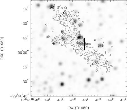
Figure 1: Image of the velocity–integrated 2.12 $\micron$ H₂ 1–0 S(1) line (contours) overlaid onto the 2MASS K-band image (greyscale). The contours are: 13, 20, 30, 45, 56 and 65 $\times 10^{-6}$ erg s^-1 cm^-2 sr^-1. The cross marks the location of OH(1720 MHz) maser A.

The line–centre velocity distribution of H₂ 1–0 S(1) emission (Fig. 2) shows a systematic velocity gradient along the H₂ bar, with the mean velocity ranging from 0 km s^-1 in the north to $-50$ km s^-1 in the south. These velocities are comparable with the average values of about $-$13 km s^-1 for the northern part and $-$35 km s^-1 for the southern part obtained from the repeated observations in June 2000. Fig. 3 shows a cut along the H₂ bar illustrating the velocity gradient. Note that the small–scale structure showing deviations of $\sim$10–15  km s^-1 probably reflects the errors in determining the velocity at each position.

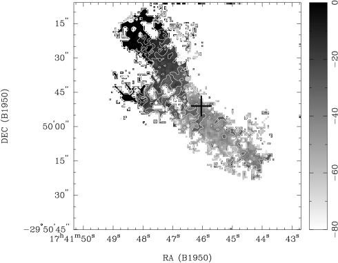
Figure 2: The line–centre velocity distribution of the 2.12 $\micron$ H₂ 1–0 S(1) line emission in both greyscale and contours. The greyscale units are in  km s^-1 and the contours are: $-5,-10,-15,-25,-35$ and $-$55 km s^-1. The cross marks the location of OH(1720 MHz) maser A.

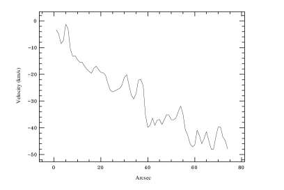
Figure 3: A cut, 5 arcsec wide, along the centre of the H₂ bar extending 80 arcsec diagonally from the top of the bar.

The presence of a star ($\rm{RA}(1950)=17^{\rm{h}}~{}41^{\rm{m}}~{}46\aas@@fstack{s}5$ , $\rm{Dec.}(1950)=-29\degr~{}49\arcmin~{}45\aas@@fstack{\prime\prime}0$) in the centre of the H₂ filament, together with the velocity difference between the north-east and south-west sections, and the jet–like appearance of the brightest H₂ contours would be consistent with a collimated bipolar jet originating from the star. However, other considerations suggest that this is unlikely. Firstly, the star in question cannot be a protostar. The 2MASS point source catalogue gives the J, H and K magnitudes of the star as $13.22\pm 0.04$, $10.31\pm 0.05$ and $8.97\pm 0.04$ respectively. Using the JHK intrinsic colours from Bessell & Brett (1988) and Koornneef (1983), and the reddening vector from Bessell & Brett (1988), we find that the extinction in K-band is $A_{K}\approx 2$ (visual extinction $A_{V}\approx 20$). These values are consistent with the lack of detection in the Digitized Sky Surveys (DSS). After correcting for extinction, we find that derived magnitudes are consistent with either a K dwarf within 100 pc of the Sun, or a K or M giant at a distance of several kpc. The former case can be excluded given that there are no molecular clouds within 200 pc of the Sun that could give rise to the H₂ emission. In the latter case the bright star is evolved and cannot be driving the outflow. The apparent location of the star at the centre of the H₂ bar is, therefore, most probably a chance alignment. Of course, it is possible that apparent outflow is being produced by a star at several kpc which is too faint to be detected. A more serious problem is that the emission does not resemble that of other outflows detected in the 1–0 S(1) line. In bipolar outflows, such as Cep E (Eisloffel et al., 1996), the emission associated with jets generally peaks in discrete knots or lobes at some distance from the driving source. Furthermore, the jets are narrow close to the driving source and the lobes have distinct, roughly constant velocities. The velocity gradient and morphology, including the extended diffuse component, present in our H₂ data are thus not consistent with entrainment by a fast, narrow protostellar jets.

Fig. 4 shows contours of velocity–integrated H₂ line emission superimposed on a 6–cm greyscale VLA image with a resolution of 12 $\aas@@fstack{\prime\prime}$7 $\times$ 8 $\aas@@fstack{\prime\prime}$2 (P.A. = 62°) (Yusef-Zadeh et al., 2001). The bar of H₂ emission is almost perpendicular to the Snake and it runs parallel to the edge of an elliptical depression located $\sim$15 arcsec to the west of the H₂ bar. The synchrotron emissivity of this depression is reduced by $\la 30$ per cent and it surrounds the Snake filament where it crosses the shell of G359.1–0.5.

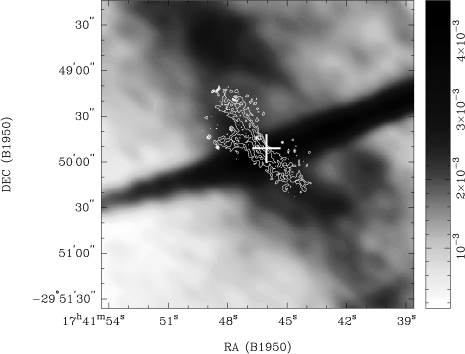
Figure 4: The velocty–integrated image of the H₂ line emission (contours) and the 6–cm radio continuum image (greyscale). The H₂ filament is located where the Snake (the dark east–west bar) crosses the shell of G359.1–0.5 (dark band extending almost north-south). The greyscale units are in Jy beam^-1 and the contours are: 13, 20, 30, 45, 56 and 65 $\times 10^{-6}$ erg s^-1 cm^-2 sr^-1. The cross marks the location of OH(1720 MHz) maser A.

3.2 Characteristics of associated molecular cloud

3.2.1 Identifying the cloud associated with G359.1–0.5

Observations of molecular clouds associated with SNRs are potentially subject to confusion due to other molecular clouds along the line of sight. However, the maser velocity of $-$5 km s^-1 can be related to the systemic velocity of the post–shock material next to the SNR shell because the OH(1720 MHz) masers are only seen in orientation where they are transverse to the motion of the expanding shock front. Hence they closely match the systemic velocity of the SNR rather than any local intrinsic expansion. We therefore expect that molecular gas with similar velocity originates from the molecular cloud associated with G359.1–0.5. In Fig. 5 we show the spectra of ¹²CO, HCO⁺, ¹³CO J=1–0 and CS J=2–1 towards maser A. In the velocity range of interest, between $-$20 and 0 km s^-1, the shape of the ¹³CO line profile differes from those of the other profiles. Inspection of the velocity cubes implies that emission within this range is most likely associated with the SNR shell. In contrast, the emission between $-$40 and $-$20 km s^-1 and the narrow features at $+$5 and $+$16 km s^-1  appear to be uncorrelated with the SNR shell or the H₂ bar.

Figure 5: ¹²CO, HCO⁺, ¹³CO J=1–0 and CS J=2–1 spectra towards maser A.

Compared with the ¹³CO spectra, the ¹²CO  and HCO⁺ spectra, and to a lesser extent the CS spectra, all show an absorption feature between $-$20 and $-5$ km s^-1. In Table 1 we list the results of a Gaussian fit to the ¹³CO feature, but for the other species affected by absorption we give only the maximum of the observed line profiles, which thus represent minimum $T_{mb}$ for these species. The correspondence between the peak of the ¹³CO emission and the centre of the absorption dip in the other three spectra implies that part of the molecular cloud is being self–absorbed in the molecular species with higher optical depth.

The overall distribution of ¹²CO, ¹³CO and CS emission show differences due to variations in optical depth across the region (the spectra of HCO⁺ were not obtained over the whole region, as the other molecules, but only towards the maser and in four positions around the maser). Maps of the emission, integrated between $-20$ and 0 km s^-1, are shown in Fig. 6 overlaid with the contours of H₂ emission. The true distribution of gas column density is represented by the ¹³CO because of its low optical depth, in contrast to the high optical depths of the other species. We note that the ¹³CO distribution is dominated by the gas located to the west of the H₂ bar. Although the ¹²CO  and CS emitting gas is covering the same region as shown by the ¹³CO map, these molecules show regions dominated by optically thin gas which is not self–absorbed, and is located east from the H₂ bar. East of the bar we thus have the gas with lower optical depth, while to the west the gas has higher optical depth. The ¹²CO  and CS maps both show an elongated feature near and parallel to the H₂ emission and the SNR shell. The H₂ bar is located at the edge of this filament of molecular gas.

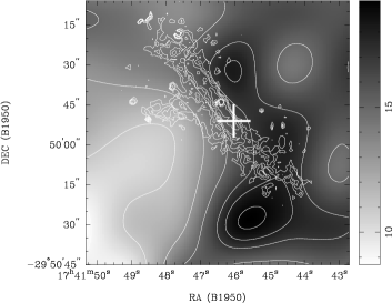
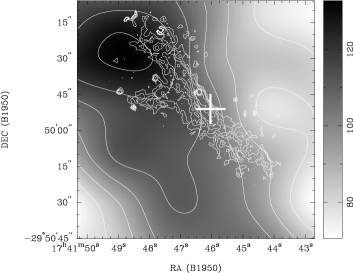
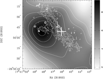
Figure 6: Maps of ¹³CO J=1–0 (upper), ¹²CO  J=1–0 (middle) and CS J=2–1 (lower) emission (shown in greyscale with matching contours) integrated between $-20$ and 0 km s^-1 overlaid with the contours of H₂ emission. The H₂ contours are: 13, 20, 30, 45, 56 and 65 $\times 10^{-6}$ erg s^-1 cm^-2 sr^-1. Contour levels (in K km s^-1) are: (¹³CO): 9, 11, 13, 15, 17, 18 and 19; (¹²CO): 70, 80, 90, 100, 110, 120 and 130; (CS): 4, 5, 6, 7, 8 and 9. The cross marks the location of the OH(1720 MHz) maser A.

3.2.2 Physical properties of the molecular cloud

Self–absorption in molecular clouds can be produced by an overlaying colder or sub–thermally excited layer. To estimate the kinetic temperature and density of the gas we have modeled the observed values of the ¹³CO J=2–1 and J=1–0 line intensities using a statistical–equilibrium excitation code supplied by J. H. Black. The code employs a mean–escape probability (MEP) approximation for radiative transfer (Jansen, van Dishoeck & Black, 1994) and calculates line intensities given kinetic temperature and density of the gas, the total column density of the molecule and the line width. For the western part of the cloud we find gas temperature of 8 $\pm$ 2 K, gas density of $10^{4}$ cm^-3, ¹³CO column density of 2.0$\times 10^{16}$ cm^-2 and ¹³CO J=1–0 optical depth of 0.3. This low optical depth is consistent with the non–detection of C¹⁸O transitions. Also, the density of $10^{4}$ cm^-3 is consistent with the molecular distribution being affected by absorption in this part of the cloud, as the lower–excitation temperatures occur at these densities for the HCO⁺ and CS lines. Using a ¹²CO/¹³CO abundance ratio of 30 (Gardner & Whiteoak, 1982) we have the ¹²CO  column density of 6.0$\times 10^{17}$ cm^-2 and ¹²CO  J=1–0 optical depth of 9. On the other hand, the eastern part of the cloud must have density $\geq$ $10^{5}$ cm^-3 because of the CS J=3–2 detection. For such densities the corresponding gas temperature derived from the code is 10 $\pm$ 2 K, ¹³CO column is $10^{16}$ cm^-2 and ¹³CO J=1–0 optical depth is 0.1. This yields a ¹²CO  column density of 3.0$\times 10^{17}$ cm^-2 and optical depth of 3.

These results show that western region of the cloud may be slightly colder than the eastern region. To investigate whether this difference in temperature is sufficient to produce the observed self–absorption, we use the following:

$$T_{abs}=f(T_{bg})e^{-\tau_{fg}}+f(T_{fg})(1-e^{-\tau_{fg}}),$$ (1)

where

$$f(T)=\frac{h\nu}{k}[(e^{\frac{h\nu}{kT}}-1)^{-1}-(e^{\frac{h\nu}{kT_{cmb}}}-1)^{-1}].$$ (2)

$T_{abs}$ is the observed temperature at the velocity of maximum absorption in ¹²CO, $T_{fg}$ is the excitation temperature of the foreground part of the cloud, $T_{bg}$ is the excitation temperature of the background part of the cloud and $\tau_{fg}$ is the optical depth of the foreground cloud. The observed $T_{abs}$ ranges from 2 to 3.3 K across the mapped region and $T_{cmb}$ = 2.7 K is the temperature of the cosmic microwave background. Using $T_{bg}$ = 10 K and $\tau_{fg}$ = 3 for the eastern part of the cloud we derive the foreground cloud excitation temperature of $T_{fg}=6\pm 1$ K. For the western part of the cloud $T_{abs}$ depends only on the excitation temperature of the foreground part of the cloud because of the high optical depth in that region ($\tau_{fg}$ = 9). Fitting the observed $T_{abs}$ we derive same $T_{fg}$ of 6 $\pm 1$ K.

The kinetic temperature of the western part of the cloud (8 $\pm$ 2 K) is in good agreement with the excitation temperature of 6 $\pm$ 1 K derived for the foreground part of the cloud. In other words, for the western part of the cloud $T_{kin}$= $T_{ex}$. Since this is the part of the cloud where ¹²CO  distribution is affected by absorption, we conclude that physically cold, not sub–thermally excited layer of the cloud is responsible for the self–absorption in the observed spectra.

4 Discussion

The H₂ 1–0/2–1 S(1) line ratio of $\sim$ 20 is consistent with shock excitation, as expected from the presence of the OH(1720 MHz) maser. Although UV excitation can, in principle, produce the 1–0 S(1) line intensity without violating the limit on the 2–1 line when molecular gas of density $10^{5}$ – $10^{6}$ cm^-3 is exposed to a FUV flux of $G_{0}\ga 10^{4.5}$ (Burton, Hollenbach & Tielens, 1990), there is no OB star within 1 pc, as evident from the 2MASS point source catalogue, there are no H ii regions apparent in the continuum map, and no significant emission in the Midcourse Space Experiment (MSX) bands at 8.3 and 21.3 µm within an arcmin of the maser.

The H₂ emission must then originate from a shock driven by the SNR. The OH(1720 MHz) maser is expected to be located within the cooling gas behind a C–type shock wave (Lockett et al., 1999), and its location just inside the sharp western edge of the H₂ emission supports the idea that the expanding shell of G359.5-0.1 is driving a shock into a molecular cloud at that location. Shock models do not predict OH column density required to produce OH(1720 MHz) masers (Draine, Roberge, & Dalgarno, 1983; Kaufman & Neufeld, 1996). Lockett et al. (1999) and Wardle (1999) suggested that the OH column density is enhanced by UV photodissocaition of H₂O. The internal FUV field generated by the X–rays from an SNR interior are able to dissociate more than 1 per cent of H₂O, which is enough to produce the required OH abundance (Wardle, 1999). How does this FUV field affects the H₂ emission? It is about 100 times weaker than the standard interstellar field (1.6$\times 10^{-3}$ erg s^-1 cm^-2), which makes it far less than that associated with an H ii region or PDR. The corresponding local X–ray energy deposition per particle is then $H_{x}/n\sim 7\times 10^{-29}$ erg cm³ s^-1 (see equation 2 from Maloney, Hollenbach, & Tielens 1996). From Fig.6a in Maloney et al. (1996) the intensity in the 2.12 $\micron$ H₂ 1–0 S(1) line of 3.2$\times 10^{-5}$ erg s^-1 cm^-2 sr^-1 which is 0.2 per cent of observed peak H₂ flux. Thus, the FUV field produced by X–rays has negligible contribution to the excitation of the 2.12 $\micron$ H₂ 1–0 S(1) line.

The H₂ bar follows the distribution of extended OH(1720 MHz) maser emission (Yusef-Zadeh et al., 1995), which is believed to be an evidence of this interaction on the global scale (Yusef-Zadeh et al., 1999). Indeed, X–ray observations (Bamba et al., 2000) show a centre–filled morphology of this SNR which, in conjunction with the shell morphology in radio band, has been proposed as a characteristic of SNRs interacting with molecular clouds (Rho & Petre, 1998). We found the H₂ emission near other masers in this SNR aligned well with the SNR shell (Lazendic et al., 2001). The magnetic field along the line of sight towards maser A was estimated to be $\sim 560\mu$G and the magnetic field was found oriented along the H₂ bar (Yusef-Zadeh, Roberts & Bower, 2001). The thickness of the shock is expected to be of order $10^{17}$ cm, about an arcsec at a distance of 8.5 kpc. We identify the sharp western edge of the bar as being the leading, limb brightened edge of a curved shock front. The maser velocity is distinct from the mean velocity of about $-$30 km s^-1 of the shocked H₂ at this location, but the maser is preferentially produced when the shock front is perpendicular to the line of sight. The H₂ velocity gradient could be the result of a pre–existing gradient, since a gradient of $\sim$5 km s^-1 is found in the ¹³CO gas in same direction.

The results derived from the molecular spectra imply the presence of a density gradient across the region, and the obvious mechanism to produce such a gradient is the passage of an SNR shock wave. The denser gas ($\sim$$10^{5}$ – $10^{6}$ cm^-3) then corresponds to post–shocked gas and the lower density gas ($\sim$$10^{4}$ cm^-3) corresponds to ambient pre–shocked gas, with the H₂ filament being the boundary between the two regions. A similar case of self–absorption by pre–shocked gas was also seen in IC 443 (White et al., 1987; van Dishoeck, Jansen, & Phillips, 1993). The values obtained for gas densities are consistent with those expected in shocks. Because of the presence of the OH(1720 MHz) maser, which requires a density $\sim$$10^{5}$ cm^-3, the pre–shock density must be $\sim$$10^{4}$ cm^-3 since the typical compression in shocks is $\sim$20–30 (for shock speed of 20–30 km s^-1 and Alfv$\acute{\rm{e}}$n speed in molecular clouds of 2 km s^-1). In Fig. 7 we present a schematic model of the SNR shock passing through the molecular cloud. Dense gas is located mostly on the eastern side of the H₂ filament, i.e. behind the shock front, while the lower density gas extends mostly to the west from the H₂ emission, i.e. in front of the shock front.

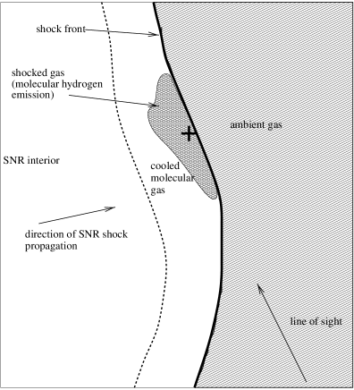
Figure 7: A schematic model of the molecular cloud towards the maser A (marked with a cross) is presented to illustrate the distribution of different components. The H₂ bar is located just behind the thin shock front, which is expanding in a direction transverse to the line of sight.

The gas temperature between the pre–shock and post–shock gas does not differ much since the gas cools rapidly behind the C–type shock. We did not detect the warm molecular gas, other than in H₂, found in other SNRs associated with OH(1720 MHz) masers (van Dishoeck, Jansen, & Phillips, 1993; Frail & Mitchell, 1998; Reach & Rho, 1999). The reason is probably beam dilution. The warm gas is less than 0.6 pc away from the shock front, as inferred from the H₂ emission, and our beam of 1–2 pc in size includes the volume of gas further away that has been cooled to near–ambient gas temperature. The post–shock/ambient cloud temperature of 10 K is consistent with the excitation temperature derived for the clouds in the Galactic Centre region (Oka et al., 1998). The beam dilution might be also the reason for non–detection of H₂CO and SiO transitions which favour regions with higher temperatures. Although the pre–shock gas temperature of $\sim$8 K is lower than typical molecular cloud temperatures of $\geq 10$ K (Goldsmith, 1987), dark clouds are found with temperatures low as this (Dickman, 1975; Snell, 1981). In our case, a likely explanation for this is the broad line width of the cloud (15 – 20 km s^-1) which enables more efficient cooling. This is supported by the results of the MEP code. As CO is the dominant coolant at densities $\sim$$10^{4}$ cm^-3 (Goldsmith & Langer, 1978), we can estimate the total cooling rate using the total power in the rotational transition of ¹²CO. For a ¹²CO  column density of $10^{18}$ cm^-2 and volume density of $10^{4}$ cm^-3, the power emitted for $\Delta v$ = 20 km s^-1 and $T_{kin}$= 8 K is $\sim$4$\times 10^{-23}$ erg s^-1 CO^-1, and for $\Delta v$ = 2 km s^-1 and $T_{kin}$= 15 K is $\sim$4.7$\times 10^{-23}$ erg s^-1 CO^-1. Thus the cooling rate from a 8 K cloud with 20 km s^-1 line width is similar to that of a 15 K cloud with a 2 km s^-1 line width.

Despite the positional coincidence and spatial proximity of the two, we did not find any morphological evidence in our data that supports the interaction between the SNR and the Snake. Similarly besides the positional coincidence, there is no obvious relationship between the H₂ emission and the Snake. In the view of the recent suggestion by Bicknell & Li (2001) that the origin of the Snake is linked to rotating molecular clouds, we examined the possibility that the velocity gradient in H₂ of $\pm$20 km s^-1 might originate from rotation of a flattened cloud. The 1–0 S(1) emission runs along an elliptical depression in the 6–cm emission from the SNR where the Snake crosses it (see Fig 4). This depression could be caused by a rotating dense molecular cloud. However, we derive the mass of the cloud from our ¹³CO data to be $\sim 700$$M_{\odot}$, in which case its escape speed is about 1.6 km s^-1 and its self–gravity could not sustain the rotation.

5 Conclusions

We carried out near–IR and millimetre wavelength observations of the region around the OH(1720 MHz) maser located at the apparent intersection of the nonthermal filament the Snake and the SNR shell G359.1–0.5. A bar of H₂ emission was found encompassing the OH(1720 MHz) maser and aligned with the SNR shell. We suggest that H₂ emission originates from the expansion of the SNR blast wave, which is evident from the sharp western edge that corresponds to the forward shock. This shocked H₂ emission, as inferred from the 1–0 and 2–1 S(1) line ratio, supports the notion that the OH(1720 MHz) masers association with SNRs are produced in molecular shock waves.

Emission from the molecular species ¹²CO, CS, HCO⁺ and ¹³CO  was detected at the maser velocity. The spectra of the former three species are affected by broad–line absorption which originates from a colder layer of molecular gas. Optically thin ¹³CO was unaffected by the absorption and is produced mostly in this colder layer, identified as pre–shocked gas. The inferred density gradient across the region places higher density post–shocked gas west of the H₂ bar. The distribution of the pre–shock and post–shock gas is consistent with the passage of the SNR shock and the H₂ bar being the boundary between the two regions.

The warm molecular gas from post–shocked gas was not detected in millimetre wavelengths probably because of beam dilution. For a better morphological and qualitative study of the shocked molecular gas towards maser A we plan to obtain observations at sub–millimetre wavelengths, which will have improved spatial resolution. Observations at other maser positions in the SNR are in progress to obtain a global view of the interaction of the SNR G359.1–0.5 with its molecular gas environment.

References

- Bamba et al. (2000) Bamba, A., Yokogawa, J., Sakano, M. & Koyama, K. 2000, PASJ, 52, 259
- Benford (1997) Benford, G. 1997, MNRAS, 285, 573
- Bessell & Brett (1988) Bessell, M. S. & Brett, J. M. 1988, PASP, 100, 1134
- Burton, Hollenbach & Tielens (1990) Burton, M. G., Hollenbach, D. J. & Tielens, A. G. G. M. 1990, ApJ, 365, 620
- Bicknell & Li (2001) Bicknell, G. V. & Li, J. 2001, ApJL, 548, L69
- Cutri (1997) Cutri, R. M. 1997, ASSL Vol. 210: The Impact of Large Scale Near-IR Sky Surveys, 187
- Dickman (1975) Dickman, R. L. 1975, ApJ, 202, 50
- Draine, Roberge, & Dalgarno (1983) Draine, B. T., Roberge, W. G., & Dalgarno, A. 1983, ApJ, 264, 485
- Eisloffel et al. (1996) Eisloffel, J., Smith, M. D., Davis, C. J., & Ray, T. P. 1996, AJ, 112, 2086
- Frail, Goss & Slysh (1994) Frail, D. A., Goss, W. M. & Slysh, V. I. 1994, ApJL, 424, L111
- Frail et al. (1996) Frail, D. A., Goss, W. M., Reynoso, E. M., Giacani, E. B., Green, A. J. & Otrupcek, R. 1996, AJ, 111, 1651
- Frail & Mitchell (1998) Frail, D. A. & Mitchell, G. F. 1998, ApJ, 508, 690
- Gardner & Whiteoak (1982) Gardner, F. F. & Whiteoak, J. B. 1982, MNRAS, 199, 23P
- Goldsmith & Langer (1978) Goldsmith, P. F. & Langer, W. D. 1978, ApJ, 222, 881
- Goldsmith (1987) Goldsmith, P. F. 1987, ASSL Vol. 134: Interstellar Processes, 51
- Gray et al. (1995) Gray, A. D., Nicholls, J., Ekers, R. D. & Cram, L. E. 1995, ApJ, 448, 164
- Green et al. (1997) Green, A. J., Frail, D. A., Goss, W. M. & Otrupcek, R. 1997, AJ, 114, 2058
- Jansen, van Dishoeck & Black (1994) Jansen, D. J., van Dishoeck, E. F. & Black, J. H. 1994, A&A, 282, 605
- Kaufman & Neufeld (1996) Kaufman, M. J. & Neufeld, D. A. 1996, ApJ, 456, 611
- Koornneef (1983) Koornneef, J. 1983, A&A, 128, 84
- Koralesky et al. (1998) Koralesky, B., Frail, D. A., Goss, W. M., Claussen, M. J., & Green, A. J. 1998, AJ, 116, 1323
- Lazendic et al. (2001) Lazendic et al. 2001, in preparation
- Lockett et al. (1999) Lockett, P., Gauthier, E. & Elitzur, M. 1999, ApJ, 511, 235
- Loren & Wootten (1980) Loren, R. B. & Wootten, A. 1980, ApJ, 242, 568
- Maloney et al. (1996) Maloney, P. R., Hollenbach, D. J., & Tielens, A. G. G. M. 1996, ApJ, 466, 561
- Nicholls & Le Strange (1995) Nicholls, J. & Le Strange, E. T. 1995, ApJ, 443, 638
- Oka et al. (1998) Oka, T., Hasegawa, T., Sato, F., Tsuboi, M. & Miyazaki, A. 1998, ApJS, 118, 455
- Reach & Rho (1999) Reach, W. T. & Rho, J. 1999, ApJ, 511, 836
- Rho & Petre (1998) Rho, J. & Petre, R. 1998, ApJL, 503, L167
- Ryder et al. (1998) Ryder, S. D., Sun, Y.-S. Ashley, M. C. B., Burton, M. G., Allen, L. E. & Storey, J. W. V. 1998, Publications of the Astronomical Society of Australia, 15, 228
- Snell (1981) Snell, R. L. 1981, ApJS, 45, 121
- Uchida, Morris & Yusef-Zadeh (1992) Uchida, K., Morris, M. & Yusef-Zadeh, F. 1992, AJ, 104, 1533
- Uchida et al. (1996) Uchida, K. I., Morris, M., Serabyn, E., & Guesten, R. 1996, ApJ, 462, 768
- van Dishoeck, Jansen, & Phillips (1993) van Dishoeck, E. F., Jansen, D. J., & Phillips, T. G. 1993, A&A, 279, 541
- Wardle (1999) Wardle, M. 1999, ApJL, 525, L101
- White et al. (1987) White, G. J., Rainey, R., Hayashi, S. S. & Kaifu, N. 1987, A&A, 173, 337
- Yusef-Zadeh et al. (1995) Yusef-Zadeh, F., Uchida, K. I. & Roberts, D. 1995, Science, 270, 1801
- Yusef-Zadeh et al. (1996a) Yusef-Zadeh, F., Roberts, D. A., Goss, W. M., Frail, D. A. & Green, A. J. 1996a, ApJL, 466, L25
- Yusef-Zadeh et al. (1996b) Yusef-Zadeh, F., Robinson, B. T., Roberts, D. A., Goss, W. M., Frail, D. A. & Green, A. 1996, The Galactic Center, Astronomical Society of the Pacific (ASP) Conference Series, Volume 102, 1996b, ed. Roland Gredel, p.151
- Yusef-Zadeh et al. (1999) Yusef-Zadeh, F., Goss, W. M., Roberts, D. A., Robinson, B., & Frail, D. A. 1999, ApJ, 527, 172
- Yusef-Zadeh, Roberts & Bower (2001) Yusef-Zadeh, F., Roberts, D. & Bower, G. 2001, Proceedings of an ASP Conference held in Brazil, March 2001, ed: Victor Migenes
- Yusef-Zadeh et al. (2001) Yusef-Zadeh et al. 2001, in preparation