The integrated Sachs-Wolfe Effect – Large Scale Structure Correlation

Abstract

We discuss the correlation between late-time integrated Sachs-Wolfe (ISW) effect in the cosmic microwave background (CMB) temperature anisotropies and the large scale structure of the local universe. This correlation has been proposed and studied in the literature as a probe of the dark energy and its physical properties. We consider a variety of large scale structure tracers suitable for a detection of the ISW effect via a cross-correlation. In addition to luminous sources, we suggest the use of tracers such as dark matter halos or galaxy clusters. A suitable catalog of mass selected halos for this purpose can be constructed with upcoming wide-field lensing and Sunyaev-Zel’dovich (SZ) effect surveys. With multifrequency data, the presence of the ISW-large scale structure correlation can also be investigated through a cross-correlation of the frequency cleaned SZ and CMB maps. While convergence maps constructed from lensing surveys of the large scale structure via galaxy ellipticities are less correlated with the ISW effect, lensing potentials that deflect CMB photons are strongly correlated and allow, probably, the best mechanism to study the ISW-large scale structure correlation with CMB data alone.

]

I Introduction

It is by now well known the importance of cosmic microwave background (CMB) temperature fluctuations as a probe of cosmology [2]. In addition to the dominant anisotropy contribution at the last scattering surface [3], CMB photons, while on transit to us, encounter the large scale structure which imprints modifications on the temperature fluctuations. In general, large scale structure affects CMB through two distinct processes: gravity and Compton scattering. The modifications due to gravity arises from frequency changes via gravitational red and blue-shifts [4, 5], through deflections involving lensing [6, 7] and time-delays [8]. During the reionized epoch, photos can both generate and erase primary fluctuations through scattering via free electrons [9, 10].

Here, we discuss an effect due to gravitational redshift commonly known in the literature as the integrated Sachs-Wolfe (ISW; [4]) effect at late times. The temperature fluctuations in the ISW effect result from the differential redshift effect from photons climbing in and out of time evolving potential perturbations from last scattering surface to the present day. In currently popular cold dark matter cosmologies with a cosmological constant, significant contributions arise at redshifts of cosmological constant domination ($z\lesssim 2$), at on and above the scale of the horizon at the time of decay. When projected on the sky, the ISW effect contributes at large angular scales and has a power spectrum that scales with the wavenumber as $k^{-5}$ times the linear density field power spectrum [11]. This is in contrast to most other contributions to CMB temperature fluctuations from the local universe, such as the well known thermal Sunyaev-Zel’dovich (SZ; [9]) effect, that peak at small angular scales and scales with the wavenumber as $k^{-1}$.

Since time evolving potentials that contribute to the ISW effect may also be probed by observations of the large scale structure, it is then expected that the ISW effect may be correlated with certain tracers. The presence of the ISW effect can then be detected via a cross-correlation of the CMB temperature fluctuations at large angular scales and the fluctuations in an appropriate tracer field. Since the ISW contribution is sensitive to how one models cosmology at late-times, such as the presence of a dark energy component and its physical properties (for example, the ratio of dark energy pressure to density), the correlation between the CMB temperature and tracer fields has been widely discussed in the literature [12].

Though several attempts have already been made to cross-correlate the ISW effect, using the best COBE temperature map, and foreground sources, such as X-ray and radio galaxies, there is, so far, no clear detection of the correlation signal [13]. As we discuss later, these non-detections are not surprising given the large sample variance associated with the correlating part of the temperature fluctuations, i.e., the ISW effect, with contribution to the variance coming from the primary temperature fluctuations. Even for the best case scenarios involving whole-sky observations and no noise contribution in the tracer field, the expected cumulative signal-to-noise for the ISW-large scale structure correlation is at most a ten. If the ISW-large scale structure correlation is to be used as probe of cosmological and astrophysical properties, it is certainly necessary to study in detail what tracers are best correlated with the ISW effect and why.

In this paper, we address this question by studying in detail the correlation between the ISW effect and large scale structure. Since we are primarily interested in understanding what types of tracers are best suited to detect the correlation, we will consider a variety of large scale structure observations and tracers. These include luminous sources such as galaxies or active galactic nuclei (AGN) at different wavelengths, the dark matter halos or galaxy clusters that describe the large scale clustering of the universe, gravitational lensing, and other contributions to CMB from the large scale structure, such as the thermal SZ effect. Unlike previous studies [14, 25], we do not consider cosmological applications of the cross-correlation involving measurement of dark matter and dark energy properties.

In § II, we outline the correlation between ISW effect and large scale structure. In § III, we discuss our results and study which tracer is best suited for correlation studies. We suggest that in addition to tracers involving sources such as galaxies or AGNs, dark matter halos that contain these sources may also be suitable for a detection of the ISW effect via a cross-correlation. The best probe of the ISW-large scale structure correlation is the lensing effect on CMB photons on transit to us from the last scattering surface. Since one can extract information related to lensing deflections from quadratic statistics on temperature data [16, 17], this allows one to use all-sky CMB anisotropy maps, such as from the Planck surveyor, alone to extract the ISW-large scale structure correlation.

II ISW-Large Scale Structure Correlation

The integrated Sachs-Wolfe effect [4] results from the late time decay of gravitational potential fluctuations. The resulting temperature fluctuations in the CMB can be written as

$$T^{\rm ISW}(\hat{\bf n})=-2\int_{0}^{r_{0}}dr\dot{\Phi}(r,\hat{\bf n}r)\,,$$ (1)

where the overdot represent the derivative with respect to conformal distance, or equivalently look-back time, from the observer at redshift $z=0$

$$r(z)=\int_{0}^{z}{dz^{\prime}\over H(z^{\prime})}\,.$$ (2)

Here, the expansion rate for adiabatic CDM cosmological models with a cosmological constant is

$$H^{2}=H_{0}^{2}\left[\Omega_{m}(1+z)^{3}+\Omega_{K}(1+z)^{2}+\Omega_{\Lambda}\right]\,,$$ (3)

where $H_{0}$ can be written as the inverse Hubble distance today $H_{0}^{-1}=2997.9h^{-1}$Mpc. We follow the conventions that in units of the critical density $3H_{0}^{2}/8\pi G$, the contribution of each component is denoted $\Omega_{i}$, $i=c$ for the CDM, $g$ for the baryons, $\Lambda$ for the cosmological constant. We also define the auxiliary quantities $\Omega_{m}=\Omega_{c}+\Omega_{b}$ and $\Omega_{K}=1-\sum_{i}\Omega_{i}$, which represent the matter density and the contribution of spatial curvature to the expansion rate respectively.

Writing multipole moments of the temperature fluctuation field $T(\hat{\bf n})$,

$$a_{lm}=\int d\hat{\bf n}T(\hat{\bf n})Y_{l}^{m}{}^{*}(\hat{\bf n})\,,$$ (4)

we can formulate the angular power spectrum as

$$\langle a_{l_{1}m_{1}}^{*}a_{l_{2}m_{2}}\rangle=\delta^{\rm D}_{l_{1}l_{2}}\delta^{\rm D}_{m_{1}m_{2}}C_{l_{1}}\,.$$ (5)

For the ISW effect, multipole moments are

$$a^{\rm ISW}_{lm} = i^{l}\int\frac{d^{3}{\bf k}}{2\pi^{2}}\int dr\dot{\Phi}({\bf k})I_{l}(k)Y_{l}^{m}(\hat{{\bf k}})\,,$$ (6)

with $I_{l}^{\rm ISW}(k)=\int drW^{\rm ISW}(k,r)j_{l}(kr)$, and the window function for the ISW effect, $W^{\rm ISW}$. Here, we have used the Rayleigh expansion of a plane wave

$$e^{i{\bf k}\cdot\hat{\bf n}r}=4\pi\sum_{lm}i^{l}j_{l}(kr)Y_{l}^{m\ast}(\hat{\bf k})Y_{l}^{m}(\hat{\bf n})\,.$$ (8)

In order to calculate the power spectrum involving the time-derivative of potential fluctuations, we make use of the cosmological Poisson equation [18]. In Fourier space, we can relate fluctuations in the potential to the density field as:

$$\Phi={3\over 2}\frac{\Omega_{m}}{a}\left({H_{0}\over k}\right)^{2}\left(1+3{H_{0}^{2}\over k^{2}}\Omega_{K}\right)^{-2}\delta(k,r)\,.$$ (9)

Thus, the derivative of the potential can be related to a derivative of the density field and the scale factor $a$. In linear theory, the density field may be scaled backwards to a higher redshift by the use of the growth function $G(z)$, where $\delta(k,r)=G(r)\delta(k,0)$ [19]

$$G(r)\propto{H(r)\over H_{0}}\int_{z(r)}^{\infty}dz^{\prime}(1+z^{\prime})\left({H_{0}\over H(z^{\prime})}\right)^{3}\,.$$ (10)

Note that in the matter dominated epoch $G\propto a=(1+z)^{-1}$. It is, therefore, convenient to define a new variable $F(r)$ such that $F\equiv G/a$.

Since we will be discussing the correlation between the ISW effect and the tracers of the large scale structure density field, for simplicity, we can write the power spectrum of ISW effect in terms of the density field such that

$$C_{l}^{\rm ISW}={2\over\pi}\int k^{2}dkP_{\delta\delta}(k)\left[I_{l}^{\rm ISW}(k)\right]^{2}\,,$$ (11)

where

$$I_{l}^{\rm ISW}(k)=\int_{0}^{r_{0}}drW^{\rm ISW}(k,r)j_{l}(kr)\,,$$ (12)

with

$$W^{\rm ISW}(k,r)=-3\Omega\left(\frac{H_{0}}{k}\right)^{2}\dot{F}\,.$$ (13)

Here, we have introduced the power spectrum of density fluctuations

$$\left<\delta({\bf k})\delta({\bf k^{\prime})}\right>=(2\pi)^{3}\delta^{\rm D}({\bf k}+{\bf k^{\prime}})P(k)\,,$$ (14)

where

$$\frac{k^{3}P_{\delta\delta}(k)}{2\pi^{2}}=\delta_{H}^{2}\left({k\over H_{0}}\right)^{n+3}T^{2}(k)\,,$$ (15)

in linear perturbation theory. Here, $\delta_{H}$ is the amplitude of the present-day density fluctuations at the Hubble scale and we use the fitting formulae of [20] in evaluating the transfer function $T(k)$ for CDM models.

The cross-correlation between the ISW effect and another tracer of the large scale structure can be similarly constructed by taking the multipole expansion of the tracer field. Following arguments similar to the above, we obtain this cross-correlation as

$$C_{l}^{{\rm ISW}-{\rm X}}={2\over\pi}\int k^{2}dkP_{\delta\delta}(k)I_{l}^{\rm ISW}(k)I_{l}^{\rm X}(k)\,,$$ (16)

where

$$I_{l}^{\rm X}(k)=\int_{0}^{r_{0}}drW^{\rm X}(k,r)j_{l}(kr)\,,$$ (17)

with the window function for the $X$-field as $W^{\rm X}(k,r)$. To estimate how well the tracer field correlates with the ISW effect, we will introduce the correlation coefficient $r_{{\rm ISW}-{\rm X}}$ such that

$$r_{{\rm ISW}-{\rm X}}=\frac{C_{l}^{{\rm ISW}-{\rm X}}}{\sqrt{C_{l}^{\rm ISW}C_{l}^{\rm X}}}\,,$$ (18)

where the power spectrum of the X-field follows

$$C_{l}^{{\rm X}}={2\over\pi}\int k^{2}dkP_{\delta\delta}(k)\left[I_{l}^{\rm X}(k)\right]^{2}\,.$$ (19)

A correlation coefficient of $\sim 1$ suggests that the tracer field is well correlated with the ISW effect. One of the goals of this paper is to investigate what tracer fields lead to correlation coefficients close to 1.

Using the covariance of the cross-correlation power spectrum, we can write the signal-to-noise for the detection of the ISW-large scale structure as

$$\left(\frac{\rm S}{\rm N}\right)^{2}=f_{\rm sky}\sum_{l=l_{\rm min}}^{l_{\rm max}}(2l+1)$$ (20)

$$\times \frac{\left[C_{l}^{{\rm ISW}-{\rm X}}\right]^{2}}{\left[C_{l}^{{\rm ISW}-X}\right]^{2}+\left(C_{l}^{\rm ISW}+C_{l}^{\rm N_{\rm ISW}}\right)\left(C_{l}^{{\rm X}}+C_{l}^{\rm N_{\rm X}}\right)}\,,$$ (21)

where noise contributions to the ISW map and the tracer map are given by $C_{l}^{\rm N_{\rm ISW}}$ and $C_{l}^{\rm N_{\rm X}}$, respectively.

In the case of the ISW effect, the noise contributions are effectively

$$C_{l}^{\rm N_{\rm ISW}}=C_{l}^{\rm CMB}+C_{l}^{\rm det}\,,$$ (22)

where $C_{l}^{\rm CMB}$ is the total temperature fluctuation contribution, including the ISW contribution, while $C_{l}^{\rm det}$ is any detector noise contribution. As we find later, it is the $C_{l}^{\rm CMB}$ that limits the signal-to-noise for the detection of the ISW-large scale structure correlation. Therefore, most of the results we present here apply equally well to both MAP and Planck surveyor missions. We will also discuss tracer fields, such as the SZ effect, involving information extracted using temperature data from these satellites. In such cases, when the signal-to-noise is different, we will separately quote them for MAP and Planck.

In equation 21, we have approximated the number of independent modes available for the measurement of the cross-correlation as $f_{\rm sky}(2l+1)$. The summation generally starts from $l_{\rm min}=2$, though, when observations are limited to a fraction of the sky, the low multipoles are not independent and there is a substantial reduction in the number of independent modes. To account for the loss of low multipole modes, one can approximate the summation such that $l_{\rm min}\sim\pi/\theta_{\rm sky}$ where $\theta_{\rm sky}$ is the survey size in smallest dimension. Since the ISW effect peaks at large angular scales, where in some cases the cross-correlation is also, it is crucial that the reduction in signal-to-noise due to partial sky coverage be considered.

Since we will be primarily interested in all-sky temperature maps from upcoming satellite missions, these issues are of minor concern. We will assume a usable fraction of $f_{\rm sky}=0.65$ for such missions due to sky cuts involving galactic plane etc, which still leads to almost independent modes at each multipole. When cross-correlating with surveys of limited area tracer fields, however, the detectability of the ISW effect via the attempted correlation may crucially depend on the sky coverage of the tracer field.

Note that an expression of the type in equation (11) can be evaluated efficiently with the Limber approximation [21]. Here, we employ a version based on the completeness relation of spherical Bessel functions

$$\int dkk^{2}F(k)j_{l}(kr)j_{l}(kr^{\prime})\approx{\pi\over 2}d_{A}^{-2}\delta^{\rm D}(r-r^{\prime})F(k)\big{|}_{k={l\over d_{A}}}\,,$$ (23)

where the assumption is that $F(k)$ is a slowly-varying function. Using this, we obtain a useful approximation for the power spectrum for sufficiently high $l$ values, $l\sim$ few hundred, as

$$C_{l}^{\rm ISW}=\int dr\frac{\left[W^{\rm ISW}\right]^{2}}{d_{A}^{2}}P_{\dot{\Phi}\dot{\Phi}}\left[k=\frac{l}{d_{A}},r\right]\,.$$ (24)

Here, the comoving angular diameter distance, in terms of the radial distance, is

$$d_{A}=H_{0}^{-1}\Omega_{K}^{-1/2}\sinh(H_{0}\Omega_{K}^{1/2}r)\,.$$ (25)

Note that as $\Omega_{K}\rightarrow 0$, $d_{A}\rightarrow r$ and we define $r(z=\infty)=r_{0}$.

Although we maintained generality in all derivations, we now illustrate our results with the currently favored $\Lambda$CDM cosmological model. The parameters for this model are $\Omega_{c}=0.30$, $\Omega_{b}=0.05$, $\Omega_{\Lambda}=0.65$ and $h=0.65$. With $n=1$, we adopt the COBE normalization for $\delta_{H}$ [22] of $4.2\times 10^{-5}$, such that mass fluctuations on the $8h$ Mpc^-1 scale is $\sigma_{8}=0.86$, consistent with observations on the abundance of galaxy clusters [23].

III Results

FIG. 1.: The signal-to-noise for the detection of source-ISW cross-correlation with a variety of sources that trace the large scale structure. The considered surveys include: HEAO X-ray catalog, radio sources from the NVSS, and the upcoming Sloan galaxy catalog. The signal-to-noise includes the fraction of sky covered in each of these surveys. The correlation with Sloan is limited by the sample variance associated with the ISW signal while the other two catalogs have significant shot-noise associated with the limited number counts.

FIG. 2.: The signal-to-noise for the detection of source-ISW cross-correlation with dark matter halos that trace the large scale structure with low mass limits down to 10¹⁵, 10¹⁴ and 10¹³ M${}_{\hbox{$\odot$}}$ (solid lines). The long-dashed line is the maximum signal-to-noise when the ISW effect can be perfectly separated from the dominant CMB data. The dot-dashed line shows an estimate for the correlation using a catalog of clusters based on the proposed Dark Universe Exploration Telescope (DUET).

We now discuss a variety of large scale structure tracers that can potentially be used to cross-correlate with CMB temperature data.

A ISW-source Correlation

Probably the most obvious tracer of the large scale structure density field in the linear regime is luminous sources such as galaxies at optical wavelengths and AGNs at X-rays and/or radio wavelengths. We can write the associated window function in this case as

$$W^{\rm X}(k,r)=b_{\rm X}(k,r)n_{\rm X}(r)G(r)\,,$$ (26)

where $b_{X}(k,r)$ is the scale-dependent source bias as a function of the radial distance and $n_{X}(r)$ is the normalized redshift distribution of sources such that $\int_{0}^{r_{0}}n_{\rm X}(r)=1$. We will model the redshift distribution in current and upcoming source catalogs with an analytic form:

$$n_{\rm X}(z)=\left(\frac{z}{z_{0}}\right)^{\alpha}\exp-\left(\frac{z}{z_{0}}\right)^{\beta}\,,$$ (27)

where $(\alpha,\beta)$ denote the slope of the distribution at low and high $z$’s, respectively with a mean given by $\sim z_{0}$. For the purpose of this calculation we take $\alpha=\beta=1$ and vary $z_{0}$ from 0.1 to 1.5 so as to mimic the expected sources from current and upcoming catalogs as well as to cover the redshift range in which ISW contributions are generally expected. Since any redshift dependence on bias can be included as a variation to the source redshift distribution, the scale dependence on bias is more important.

Since the ISW effect is primarily associated with large linear scales, the source bias can be well approximated as scale independent. Such an assumption is fully consistent with results from numerical simulations [24], results from redshift surveys [25] and semi-analytic calculations involving the so-called halo model [26]. We take the source bias to be in the range of 1 to 3 as expected for galaxies and biased sources as X-ray objects. Since $C_{l}^{{\rm ISW}-{\rm X}}\propto b$, and $C_{l}^{\rm X}\propto b^{2}$, note that the correlation coefficient is independent of bias and other normalizing factors. The bias becomes only important for estimating the signal-to-noise.

In order to estimate signal-to-noise, we describe the noise contribution associated with source catalogs by the finite number of sources one can effectively use to cross-correlate with temperature data. We can write this shot-noise contribution as

$$C_{l}^{\rm N_{\rm X}}=\frac{1}{\bar{N}}$$ (28)

where $\bar{N}$ is the surface density of source per steradian.

In figure 1, we show cumulative signal-to-noise for a cross-correlation of the temperature data with large scale structure. We have considered three source catalogs here involving the HEAO X-ray catalog ($f_{s}ky=1/3$,$\bar{N}\sim 10^{3}$ sr^-1 and $b_{\rm X}=3$), NVSS radio sources ($f_{s}ky=0.82$,$\bar{N}\sim 2\times 10^{5}$ sr^-1 and $b_{X}=1.6$) [27] and galaxy counts down to R band magnitude of 25 from the Sloan Digital Sky survey ($f_{\rm sky}=0.25$, $7\times 10^{8}$ sr^-1 and $b_{\rm X}=1$) [28]. The first two catalogs have already been used for this cross-correlation with the COBE data [13]. The non-detection of the cross-correlation is not surprising given that we find cumulative signal-to-noise values less than 1; this estimate will become worse once the noise contribution associated with COBE temperature data is also included. In both cases, the shot-noise associated with tracer fields is significant. For Sloan, the limiting factor in the signal-to-noise is the large noise contribution associated with the ISW contribution due to dominant primary temperature fluctuations. Our estimates for the signal-to-noise for ISW-Sloan correlation is consistent with previous estimates [14], where it was concluded that the detection may be challenging given the small signal-to-noise.

In addition to luminous sources, one can also cross-correlate the temperature map with a catalog of galaxy clusters, or dark matter halos. It is expected that wide-field galaxy lensing surveys and small-angular resolution SZ surveys will allow mass selected catalogs of clusters [29]. Similar catalogs of clusters can also be compiled through wide-field galaxy catalogs such as Sloan and X-ray imaging data, such as from the proposed Dark Universe Exploration Telescope (DUET).

The redshift distribution of halos in such catalogs follows simply from analytical arguments, such as through the mass function $dn(M,z)/dM$ calculated following analytical methods such as the Press-Schechter (PS; [30]) mass function or numerical measurements [31]. Additionally, the halo bias is also well known through analytical methods [32]:

$$b_{h}(M,z)=1+\frac{\left[\nu^{2}(M,z)-1\right]}{\delta_{c}}\,,$$ (29)

where $\nu(M,z)=\delta_{c}/\sigma(M,z)$ is the peak-height threshold. $\sigma(M,z)$ is the rms fluctuation within a top-hat filter at the virial radius corresponding to mass $M$, and $\delta_{c}$ is the threshold overdensity of spherical collapse. Useful fitting functions and additional information on these quantities could be found in [33]. For the purpose of this calculation, we use $b_{X}=\langle b_{M}\rangle$, such that the mass averaged halo bias, as a function of redshift is:

$$\left<b_{M}\right>(z)=\frac{1}{\bar{n}_{h}(z)}\int_{M_{\rm min}}^{\infty}dM\frac{dn(M,z)}{dM}b_{h}(M,z)\,.$$ (30)

Here, the mean number density of halos, as a function of redshift, given by $\bar{n}_{h}(z)=\int dMdn(M,z)/dM$.

The redshift distribution of halos follow similarly from PS theory:

$$n_{\rm X}(z)=\frac{1}{\bar{N}}\frac{d^{2}V}{dzd\Omega}\left[\int_{M_{\rm min}}^{\infty}dM\frac{dn(M,z)}{dM}\right]\,,$$ (31)

where

$$\bar{N}=\int dz\frac{d^{2}V}{dzd\Omega}\left[\int_{M_{\rm min}}^{\infty}dM\frac{dn(M,z)}{dM}\right]\,,$$ (32)

with the comoving volume element given by $d^{2}V/dzd\Omega$. Note that the shot-noise associated with the halo-halo power spectrum is given by the surface-density of halos $C_{l}^{\rm N_{\rm X}}\equiv 1/\bar{N}$. Note that even though the surface density of halos are significantly smaller than, say, the case for galaxies or sources, one gains an equivalent factor with the increase in halo bias relative to the same for galaxies. Therefore, on average, we expect catalogs based on halos to produce same order of magnitude signal-to-noise as for luminous sources.

In figure 2, we show the cumulative signal-to-noise for detecting the ISW-halo correlation. Here, we assume all-sky catalogs of clusters down to a minimum mass limit of 10¹³, 10¹⁴ and 10¹⁵ M${}_{\hbox{$\odot$}}$. The lower limit of 10¹⁴ M${}_{\hbox{$\odot$}}$ is consistent with the expected mass threshold for SZ clusters that will be detected with the planned South Pole Telescope [29]. This mass limit is constant over a wide range in redshift, while mass catalogs based on lensing surveys contain a redshift dependent minimum mass limit due to the variation in the lensing window function.

The decrease in signal-to-noise with increase in mass is due to the decrease in the surface density of halos and thus the increase in the shot-noise associated with the halo side of the correlation. Though the halo surface density decreases as a function of mass, this is partly accounted by the increase in the halo bias such that even with a low surface density of halos, one can attempt a correlation of the temperature with cluster catalogs. As an example of a temperature-source catalog correlation that can be expected with the MAP data, we also show an estimate for the signal-to-noise for a catalog of $\sim$ 18000 clusters that is expected to be compiled from the wide-field X-ray survey by the proposed DUET mission (dot-dashed line). Though the cumulative signal-to-noise is below 2, the DUET catalog is significantly preferred over the Sloan survey due to the fact that cluster bias associated with DUET tracers can be a priori known through mass estimates based on the electron temperature data while galaxy bias may be more complicated.

FIG. 3.: Left: The cross-correlation power spectrum between the ISW and SZ effects. For comparison, we also show the power spectra of ISW and SZ effects and the CMB anisotropies. Right: The cumulative signal-to-noise for the detection of the ISW-SZ correlation with Planck and MAP data and using spectral dependence of the SZ contribution to separate it out from thermal CMB fluctuations. The maximum signal-to-noise is when the ISW effect is separated from the dominant primary fluctuations at the last scattering surface.

B ISW-SZ Correlation

Following the derivation of the ISW-large scale structure correlation, we can also consider the cross-correlation between the ISW effect and the Sunyave-Zel’dovich thermal effect [9] due to inverse-Compton scattering of CMB photons via hot electrons. The temperature decrement due to the SZ effect can be written as the integral of pressure along the line of sight

$$y\equiv\frac{\Delta T}{T_{\rm CMB}}=g(x)\int dra(r)\frac{k_{B}\sigma_{T}}{m_{e}c^{2}}n_{e}(r)T_{e}(r)\,$$ (33)

where $\sigma_{T}$ is the Thomson cross-section, $n_{e}$ is the electron number density, $r$ is the comoving distance, and $g(x)=x{\rm coth}(x/2)-4$ with $x=h\nu/k_{B}T_{\rm CMB}$ is the spectral shape of SZ effect. At Rayleigh-Jeans (RJ) part of the CMB, $g(x)=-2$. For the rest of this paper, we assume observations in the Rayleigh-Jeans regime of the spectrum. Due to the spectral dependence of the SZ effect when compared to CMB thermal fluctuations, the SZ signal can be extracted from CMB fluctuations in multifrequency data [35]. Here, we use expected results from such a frequency separation with Planck and MAP data, and consider the ISW-SZ cross-correlation by correlating the CMB and SZ maps. When calculating signal-to-noise, we will use the noise power spectra calculated in [35] for the Planck SZ and CMB maps.

Following our discussion on the ISW-large scale structure correlation, we can write the relevant window function for the SZ effect as

$$W^{\rm SZ}(r)=g(x)\frac{k_{B}\sigma_{T}b_{g}(r)\bar{n}_{e}}{a(r)^{2}m_{e}c^{2}}$$ (34)

where, at linear scales corresponding to the ISW effect, the pressure bias, $b_{g}$, relative the density field follows from arguments based on the halo approach to large scale pressure fluctuations [26, 34]:

$$b_{g}(z)=\int dM\frac{M}{\bar{\rho}}\frac{dn(M,z)}{dM}b_{\rm halo}(M,z)T_{e}(M,z)\,.$$ (35)

Here, $T_{e}(M,z)$ is the electron temperature, which can be calculated through arguments related to the virial theorem. In Eq. 34, $\bar{n}_{e}$ is the mean density of electrons today.

In figure 3, we show the cross-correlation between the ISW and SZ effects. For comparison, we also show the ISW and SZ power spectra. The correlation coefficient for the ISW-SZ effect ranges from 0.3, at $l\sim$ few tens to 0.1 at $l\sim$ few hundred suggesting that ISW and the SZ contributions are not strongly correlated. This could be understood based on the fact that contributions to the SZ effect primarily comes from the so-called 1-halo term of the halo models of non-linear clustering and not the 2-halo term that tracers the large scale correlations and, thus, the linear density fluctuations responsible for the ISW effect.

In the same figure, we also show the signal-to-noise for the detection of the ISW-SZ cross-correlation. For an experiment like Planck, we find that the signal-to-noise ratio is at the level of $\sim$ 4, while for MAP, it is at the level of 0.3; this is understandable as MAP has no high frequency information for a reliable separation of the SZ effect. In order to investigate what limits the signal-to-noise for the detection of the ISW-SZ correlation with a mission like Planck, we decided to set the noise contribution to the ISW effect as simply due to the ISW effect itself, instead of the total CMB power spectrum. This led to the dot-dashed line. Further removing the noise contribution to the SZ map, such that a perfect separation of the SZ effect is possible led to the dotted line, which converges to the previous dot-dashed line by $l\sim 10$. It is clear that the dominant noise contribution comes from the noise associated with the ISW effect, and effectively, the dominant CMB anisotropies at the last scattering which cannot be easily separated from the ISW effect. If there is a useful separation scheme to extract the ISW contribution alone, the expected signal-to-noise for the ISW-SZ correlation is at the level of $\sim$ 60 suggesting a clear detection of the correlation which can be used for cosmological and astrophysical purposes.

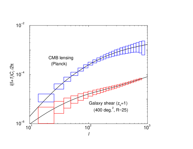
FIG. 4.: The power spectrum of convergence constructed from CMB deflections (top curve) and galaxy shape data (bottom curve). In the case of reconstruction based on CMB, we show expected errors from the Planck mission while for large scale structure weak lensing, we show expected errors for a survey of 400 deg.² down to a R band magnitude of 25.

C ISW-lensing correlation

We can consider two forms of lensing: the potentials that deflect CMB photons and potentials that shear background galaxy images. The former can be constructed using quadratic statistics in temperature data or using Fourier space statistics that are optimized to extract the lensing signal, while the latter is probed in weak lensing survey using galaxy shapes.

The deflection angle of CMB photons on the sky, $\alpha(\hat{\bf n})=\nabla\phi(\hat{\bf n})$, are given by the gradient of the projected potential $\Phi$ (see e.g. [36]),

$$\phi(\hat{\bf m}) = -2\int_{0}^{r_{0}}dr\frac{d_{A}(r_{0}-r)}{d_{A}(r)d_{A}(r_{0})}\Phi(r,\hat{{\bf m}}r)\,.$$ (36)

The lensing potential can be related to the well known convergence generally encountered in conventional lensing studies involving galaxy shear

$$\kappa(\hat{\bf m}) = {1\over 2}\nabla^{2}\phi(\hat{\bf m})$$ (37)

$$= -\int_{0}^{r_{0}}dr\frac{d_{A}(r)d_{A}(r_{0}-r)}{d_{A}(r_{0})}\nabla_{\perp}^{2}\Phi(r,\hat{{\bf m}}r)\,,$$ (38)

where note that the 2D Laplacian operating on $\Phi$ is a spatial and not an angular Laplacian. Expanding the lensing potential to Fourier moments,

$$\phi(\hat{\bf n})=\int\frac{d^{2}{\bf l}}{(2\pi)^{2}}\phi({\bf l}){\rm e}^{i{\bf l}\cdot\hat{\bf n}}\,,$$ (40)

we can write the usually familiar quantities of convergence and shear components of weak lensing as [7]

$$\kappa(\hat{\bf n}) = -\frac{1}{2}\int\frac{d^{2}{\bf l}}{(2\pi)^{2}}l^{2}\phi({\bf l}){\rm e}^{i{\bf l}\cdot\hat{\bf n}}$$ (41)

$$\gamma_{1}(\hat{\bf n})\pm i\gamma_{2}(\hat{\bf n}) = -\frac{1}{2}\int\frac{d^{2}{\bf l}}{(2\pi)^{2}}\ l^{2}\phi({\bf l}){\rm e}^{\pm i2(\phi_{l}-\phi)}{\rm e}^{i{\bf l}\cdot\hat{\bf n}}\,.$$ (42)

Though the two terms $\kappa$ and $\phi$ contain differences with respect to radial and wavenumber weights, these differences cancel with the Limber approximation [21]. In particular, their spherical harmonic moments are simply proportional

$$\phi_{lm} = -{2\over l(l+1)}\kappa_{lm}=\int d{\hat{\bf n}}Y_{l}^{m}{}^{*}(\hat{\bf n})\phi(\hat{\bf n})$$ (43)

$$= i^{l}\int{d^{3}{\bf k}\over 2\pi^{2}}\delta({\bf k})Y_{l}^{m}{}^{*}(\hat{\bf k})I_{\ell}^{\rm len}(k)$$ (44)

with

$$I_{\ell}^{\rm len}(k) = \int W^{\rm len}(k,r)j_{l}(kr)\,,$$ (45)

$$W^{\rm len}(k,r) = -3\frac{\Omega_{m}}{a}\left({H_{0}\over k}\right)^{2}G(r){d_{A}(r_{0}-r)\over d_{A}(r)d_{A}(r_{0})}\,.$$ (46)

Here, we have used the Rayleigh expansion of a plane wave, equation (8), and the fact that $\nabla^{2}Y_{l}^{m}=-l(l+1)Y_{l}^{m}$.

FIG. 5.: The signal-to-noise for the detection of lensing-ISW cross-correlation with galaxy shear data and using deflections in the CMB. The dotted lines are for galaxy weak lensing surveys with background sources at redshifts of 0.5 and 1.5, respectively, and with a sky area of $\pi$ steradians, similar to the Sloan survey. The dashed lines show the signal-to-noise when temperature data is cross-correlated with an estimator for lensing deflections in Planck and MAP temperature data. The solid line is when a temperature map is cross-correlated with a noise-free estimator of deflections.

For the construction of deflection angles based on the CMB temperature data, we make use the quadratic statistic proposed by [17] involving the divergence of the temperature weighted temperature gradients, $\nabla\cdot(\theta\nabla\theta)$. In Fourier space, we can write the estimator for the deflection angles as

$$D({\bf l}) = \frac{N_{l}}{l}\int\frac{d^{2}{\bf l}_{1}}{(2\pi)^{2}}\left({\bf l}\cdot{\bf l}_{1}C_{l_{1}}^{\rm CMB}+{\bf l}\cdot({\bf l}-{\bf l}_{1})C_{|{\bf l}-{\bf l}_{1}|}^{\rm CMB}\right)$$ (48)

$$\quad\times\frac{\theta(l_{1})\theta(|{\bf l}-{\bf l}_{1}|)}{2C_{l_{1}}^{\rm tot}C_{|{\bf l}-{\bf l}_{1}|}^{\rm tot}}\,.$$

The ensemble average, $\langle D({\bf l})\rangle$, is equal to the deflection angle, $l\phi({\bf l})$, when

$$N_{l}^{-1}=\frac{1}{l^{2}}\int\frac{d^{2}{\bf l}_{1}}{(2\pi)^{2}}\frac{\left({\bf l}\cdot{\bf l}_{1}C_{l_{1}}^{\rm CMB}+{\bf l}\cdot({\bf l}-{\bf l}_{1})C_{|{\bf l}-{\bf l}_{1}|}^{\rm CMB}\right)^{2}}{2C_{l_{1}}^{\rm tot}C_{|{\bf l}-{\bf l}_{1}|}^{\rm tot}}\,.$$ (49)

Note that $N_{l}$ is the noise power spectrum associated with the reconstructed deflection angle power spectrum:

$$\langle D({\bf l})D({\bf l}^{\prime})\rangle=(2\pi)^{2}\delta_{D}({\bf l}+{\bf l}^{\prime})\left(l^{2}C_{l}^{\phi\phi}+N_{l}\right)\,.$$ (50)

In the case of lensing surveys using galaxy shear data, we rewrite equations (42) and (46) such that $d_{A}(r_{0})=d_{A}(r_{s})$ where $r_{s})$ is radial distance to background sources from which shape measurements are made. We assume that all sources are at the same redshift, though,a distribution of sources in the redshift range expected does not lead to a significantly different result than the one suggested here.

The shot-noise contribution to the convergence power spectrum associated with lensing surveys involving galaxy ellipticity data is

$$C_{l}^{\rm N_{\rm X}}=\frac{\langle\gamma_{\rm int}^{2}\rangle}{\bar{n}}\,,$$ (51)

where $\langle\gamma_{\rm int}^{2}\rangle^{1/2}$ is the rms noise per component introduced by intrinsic ellipticities, typically $\sim$ 0.6 for best ground based surveys, and $\bar{n}$ is the surface number density of background source galaxies from which shape measurements can be made. For surveys that reach a limiting magnitude in $R\sim 25$, the surface density is consistent with $\bar{n}\sim 6.9\times 10^{8}$ sr^-1 or $\approx 56$ gal arcmin^-2 [37], such that $C_{l}^{\rm N}\sim 2.3\times 10^{-10}$.

In figure 4, we compare the lensing convergence power spectrum associated with CMB (top curve) and a large scale structure weak lensing survey from galaxy ellipticities with background source galaxies at a redshift of one. Note that we have obtained the convergence power spectrum associated with lensing deflections in CMB following the estimator for the lensing deflection power spectrum and the two are simply related following equation (42) such that $C_{l}^{\kappa}=l^{4}/4C_{l}^{\phi\phi}$. For comparison, we also show expected error bars on the reconstructed convergence power spectrum from CMB, via the Planck temperature data, and for a wide-field survey of 400 deg.² down to a R-band magnitude of 25.

In figure 5, we show the associated cumulative signal-to-noise in the detection of the ISW-lensing correlation for galaxy lensing surveys and using CMB data. We assume an area of $\pi$ steradians for the lensing surveys and as the signal-to-noise scales as $f_{\rm sky}^{1/2}$, we do not expect a significant use of the current and upcoming lensing surveys which are restricted to at most few hundred sqr. degrees. The dedicated instruments, such as the Large-aperture Synoptic Survey Telescope (LSST; [38]) however, will provide wide-area maps of the lensing convergence and these will certainly be useful for cross-correlation studies with CMB to extract the ISW effect.

Note that the Planck data allow the best opportunity to detect the ISW effect by correlating an estimator for deflections with a temperature map. The MAP has a lower cumulative signal-to-noise due to its estimator of deflections is affected by the low resolution of the temperature data. Nevertheless, the MAP data will certainly allow the first opportunity to detect the presence of the ISW effect either from CMB data alone or through cross-correlation of other tracers.

FIG. 6.: The correlation-coefficient for ISW-large scale structure correlations involving lensing effect on CMB (solid line), a catalog of dark matter halos down to a mass limit of $10^{14}$ M${}_{\hbox{$\odot$}}$ at all redshifts (dotted line), lensing convergence from galaxy shear data (dashed lines) with sources at redshifts of 0.5 and 1.5, and sources as tracers with mean redshifts of 0.4, 0.7 and 1.3. The potentials that deflect CMB photons and sources at $z\sim 1.5$ are best correlated with the ISW effect.

FIG. 7.: The contribution to the power spectra of ISW effect and other tracers as indicated. The sources have a mean redshift, $z_{0}$ of 0.4, 0.7 and 1.3 (from top to bottom). The plot shows that the contribution to the lensing effect on CMB comes from same Fourier modes as the ISW effect while there is a mismatch when compared to galaxy surveys at low redshifts.

IV Summary

We discussed the correlation between late-time integrated Sachs-Wolfe (ISW) effect in the cosmic microwave background (CMB) temperature anisotropies and the large scale structure of the local universe. This correlation has been proposed and studied in the literature as a probe of the dark energy and its physical properties. We considered a variety of large scale structure tracers suitable for a detection of the ISW effect via a cross-correlation.

We summarize our results for the correlation coefficient in figure 6. As shown, the potentials that deflect CMB photons are strongly correlated with the ISW effect with correlation coefficients of order 0.95 at multipoles of $\sim$ 10. The convergence maps constructed from galaxy shear data are not strongly correlated due to mismatches in their window function and that of the ISW effect. While catalogs of dark matter halos, or galaxy clusters, are well correlated with the ISW effect, sources at low redshifts necessarily not. Increasing the mean source redshift to $\sim$ 1.5, we find correlation coefficients of $\sim$ 0.9 suggesting that a catalog of sources at such high redshifts are preferred over a low redshift survey. Such catalogs can be constructed from surveys at X-ray and radio wavelengths, however, the surface density of such sources are significant lower than optical galaxies and the resulting cumulative signal-to-noise is subsequently smaller.

In order to understand the correlation between ISW effect and tracers, we rewrite equation (11) in the form $\int dk/kk^{3}H(k)$. In figure 7, we show $k^{3}H(k)$ as a function of $k$ for large scale structure tracers involving sources and the ISW effect. For comparison, we also show the contribution to potential power spectrum that deflect CMB photons. As shown, there is a mismatch between the wave numbers that contribute to the galaxy clustering, at low redshifts, when compared to the ISW effect. With increase in source redshift, the mismatch decreases and the sources tend to be more correlated with the ISW effect. On the other hand, it is clear that lensing potentials that deflect CMB photons are well correlated with the ISW effect. In fact, we find that the Planck survey data alone provide the best opportunity to extract the ISW effect using an estimator of lensing deflections on its temperature data. With multifrequency data, the presence of the ISW-large scale structure correlation can also be investigated through a cross-correlation of the frequency cleaned SZ and CMB maps.

In the near term, the ISW-tracer correlation is best studied through catalogs of clusters selected based on mass. Such catalogs can be constructed with upcoming wide-field lensing, SZ effect and X-ray imaging surveys. The combined DUET cluster catalog and the MAP data will allow a good opportunity to study the ISW-large scale structure correlation while the MAP data can also be used with the Sloan catalog of galaxies. We estimate signal-to-noise of order few for these scenarios suggesting that any such detection will be challenging. For DUET, attempts to improve the shot-noise on the X-ray side will be necessary while for Sloan, one should carefully select a subsample of high redshift galaxies, say through photometric redshift data.

- [1]
- [2] L. Knox, Phys. Rev. D, 52 4307 (1995); G. Jungman, M. Kamionkowski, A. Kosowsky and D.N. Spergel, Phys. Rev. D, 54 1332 (1995); J.R. Bond, G. Efstathiou and M. Tegmark, MNRAS, 291 L33 (1997); M. Zaldarriaga, D.N. Spergel and U. Seljak, Astrophys. J., 488 1 (1997); D.J. Eisenstein, W. Hu and M. Tegmark, Astrophys. J., 518 2 (1999)
- [3] W. Hu, N. Sugiyama and J. Silk, Nature, 386, 37 (1997); P. J. E. Peebles and J. T. Yu, Astrophys. J., 162, 815 (1970); R. A. Sunyaev and Ya.B. Zel’dovich, Astrophys. Space Sci. 7, 3 (1970); J. Silk, Astrophys. J., 151, 459 (1968); see recent review by W. Hu & S. Dodelson, Ann. Rev. Astro. Astrop., in press, astro-ph/0110414 (2001).
- [4] R. K. Sachs and A. M. Wolfe, Astrophys. J., 147 73 (1967)
- [5] M. J. Rees and D. N. Sciama, Nature, 519, 611 (1968) U. Seljak, Astrophys. J., 460 549 (1996); also, R. Tuluie and P. Laguna, Astrophys. J., 445 73 (1995); R. Tuluie, P. Laguna and P. Anninos, Astrophys. J., 463 15 (1996); A. Cooray, Phys. Rev. Dsubmitted (astro-ph/0109162).
- [6] A. Blanchard and J. Schneider, A&A, 184, 1 (1987); A. Kashlinsky, Astrophys. J., 331, L1 (1988); E. V. Linder, A&A, 206, 1999, (1988); S. Cole and G. Efstathiou, MNRAS, 239, 195 (1989); M. Sasaki, MNRAS, 240, 415 (1989); K. Watanabe and K. Tomita, Astrophys. J., 370, 481 (1991); M. Fukugita, T. Futumase, M. Kasai and E. L. Turner, Astrophys. J., 393, 3 (1992); L. Cayon, E. Martinez-Gonzalez and J. Sanz, Astrophys. J., 413, 10 (1993); U. Seljak, Astrophys. J., 463 1 (1996); M. Zaldarriaga and U. Seljak, Phys. Rev. D, 58 023003 (1998);
- [7] W. Hu, Phys. Rev. D, 62 043007 (2000);
- [8] W. Hu and A. Cooray, Phys. Rev. D, 63 023504 (2000)
- [9] R. A. Sunyaev and Ya. B. Zel’dovich, MNRAS, 190 413 (1980)
- [10] J. P. Ostriker and E. T. Vishniac, Nature, 322, 804 (1986); E. T. Vishniac, Astrophys. J., 322, 597 (1987); S. Dodelson and J. M. Jubas, Astrophys. J., 439, 503 (1995); G. Efstathiou, in Large Scale Motions in the Universe. A Vatican Study Week, ed. V. C. Rubin & G. V. Coyne (Princeton: Princeton University Press), 299 (1988); A. H. Jaffe and M. Kamionkowski, Phys. Rev. D, 58, 043001 (1998); W. Hu, Astrophys. J., 529, 12 (1999).
- [11] W. Hu and N. Sugiyama, Phys. Rev. D, 50, 627 (1994).
- [12] R. Crittenden and N. Turok, Phys. Rev. Lett., 76, 575 (1996); A. Kinkhabwala and M. Kamionkowski, Phys. Rev. Lett., 82, 4172 (1999).
- [13] S. Boughn, R. Crittenden and N. Turok, New Astronomy, 3, 275 (1998); S. Boughn and R. G. Crittenden, preprint (astro-ph/0111281).
- [14] H. V. Peiris and D. N. Spergel, 2000, Astrophys. J., 540, 605 (2000);
- [15] L. Verde and D. N. Spergel, preprint (astro-ph/0108179); W. Hu, preprint (astro-ph/0108090).
- [16] U. Seljak and M. Zaldarriaga, Phys. Rev. D, 60, 043504 (1999); U. Seljak and M. Zaldarriaga, Phys. Rev. Lett., 82, 2636 (1999); M. Zaldarriaga and U. Seljak, Phys. Rev. D, 59, 123507 (1999); J. Guzik, U. Seljak and M. Zaldarriaga, Phys. Rev. D, 62, 043517 (2000); K. Benabed, F. Bernardeau and L. van Waerbeke, Phys. Rev. D, 63, 043501 (2001); W. Hu, Phys. Rev. D, 64, 083005 (2001). W. Hu and T. Okamato, preprint (astro-ph/0111606)
- [17] W. Hu, Astrophys. J., 557, 79 (2001).
- [18] J. M. Bardeen, Phys. Rev. D, 22 1882 (1980)
- [19] P. J. E. Peebles, The Large-Scale Structure of the Universe, (Princeton: Princeton Univ. Press, 1980)
- [20] D. J. Eisenstein and W. Hu, Astrophys. J., 511 5 (1999)
- [21] D. Limber, Astrophys. J., 119 655 (1954)
- [22] E. F. Bunn and M. White, Astrophys. J., 480 6 (1997)
- [23] P. T. P. Viana and A. R. Liddle MNRAS, 303 535 (1999)
- [24] A. J. Benson, S. Cole, C. S. Frenk, C. M. Baugh, C. G. Lacey, MNRAS, 311, 793 (2000).
- [25] L. Verde, A. F. Heavens, M. J. Percival et al., preprint (astro-ph/0112161); H. A. Feldman, J. A. Frieman, J. N. Fry and R. Scoccimarro, Phys. Rev. Lett., 86, 1434 (2001).
- [26] R. J. Scherrer and E. Bertschinger, Astrophys. J.381, 349 (1991); R. K. Sheth and B. Jain, MNRAS, 285 231 (1997); U. Seljak, MNRAS, 318 203 (2000); C.-P. Ma and J. N. Fry, Astrophys. J., 543 503 (2000); A. Cooray and W. Hu, Astrophys. J., 548 7 (2001); R. Scoccimarro, R. Sheth, L. Hui and B. Jain, Astrophys. J., 546 20 (2001); J. A. Peacock and R. E. Smith, MNRAS, 318, 1144 (2000).
- [27] J. J. Condon, W. D. Cotton, E. W. Greisen et al. Astron. J., 115, 1693 (1998).
- [28] D. G. York, J. Adelman, J. E. Anderson, et al. Astron. J., 120, 1579 (2000).
- [29] For example, G. P. Holder, Z. Haiman and J. Mohr, Astrophys. J., 553, 545.
- [30] W. H. Press and P. Schechter, Astrophys. J., 187, 425 (1974); R. K. Sheth and G. Tormen, MNRAS, 308, 119 (1999).
- [31] A. Jenkins, C. S. Frenk, S. D. M. White, J. M. Colberg, S. Cole, A. E. Evrard, H. M. P. Couchman, N. Yoshida, MNRAS, 321, 372 (2001).
- [32] H. J. Mo, Y. P. Jing, S. D. M. White, MNRAS, 284, 189 (1997); H. J. Mo, S. D. M. White, MNRAS, 282, 347 (1996).
- [33] J. P. Henry, Astrophys. J., 534, 565 (2000); V. R. Eke, S. Cole and C. S. Frenk, MNRAS, 282, 263 (1996); T. T. Nakamura and Y. Suto, Prog. in Theor. Phys. 97, 49 (1997).
- [34] A. Cooray, 2001, Ph.D. thesis, University of Chicago, Chicago (2001); available from the U. of Chicago Crear Science Library or from the author; A. Cooray, Phys. Rev. D., in press (astro-ph/0105063)
- [35] A. Cooray, W. Hu and M. Tegmark, Astrophys. J., 540 1 (2000)
- [36] N. Kaiser, Astrophys. J., 388, 286 (1992); N. Kaiser, Astrophys. J., 498, 26 (1998); M. Bartelmann & P. Schneider, Physics Reports in press, astro-ph/9912508 (2000).
- [37] I. Smail, S. W. Hogg, L. Yan and J. G. Cohen, Astrophys. J., 449, 105 (1995).
- [38] A. Tyson and R. Angel The Large-Aperture Synoptic Survey Telescope, in “New Era of Wide-Field Astronomy”, ASP Conference Series (2000).