Maximum-entropy weak lens reconstruction: improved methods and application to data

Abstract

We develop the maximum-entropy weak shear mass reconstruction method presented in earlier papers by taking each background galaxy image shape as an independent estimator of the reduced shear field and incorporating an intrinsic smoothness into the reconstruction. The characteristic length scale of this smoothing is determined by Bayesian methods. Within this algorithm the uncertainties due to both the intrinsic distribution of galaxy shapes and galaxy shape estimation are carried through to the final mass reconstruction, and the mass within arbitrarily shaped apertures can be calculated with corresponding uncertainties. We apply this method to two clusters taken from $n$-body simulations using mock observations corresponding to Keck LRIS and mosaiced HST WFPC2 fields. We demonstrate that the Bayesian choice of smoothing length is sensible and that masses within apertures (including one on a filamentary structure) are reliable, provided the field of view is not too small. We apply the method to data taken on the cluster MS1054-03 using the Keck LRIS (Clowe et al. 2000) and HST (Hoekstra et al. 2000), finding results in agreement with this previous work; we also present reconstructions with optimal smoothing lengths, and mass estimates which do not rely on any assumptions of circular symmetry. The code used in this work (LensEnt2) is available from the web.

1 Introduction

Weak lensing studies of clusters of galaxies are an important complement to X-ray, Sunyaev-Zel’dovich effect and optical observations, allowing the projected distribution of mass to be investigated without any dynamical assumptions. The reconstruction of cluster mass distributions from weak gravitational lensing data is now well established; it has been shown that the projected density distribution can be recovered from magnification data, in the form of background galaxy number densities [Broadhurst et al. 2001, Dye & Taylor 1998], or from shear data, the net statistical distortion of the images of background galaxies [Tyson et al. 1990, Kaiser & Squires 1993, Schneider & Seitz 1995, Squires & Kaiser 1996].

We focus here on shear data, primarily because of its greater abundance; the likelihood function for shear data is also better understood (Section 2). Schneider, King and Erben [Schneider et al. 2000] discuss the use of the two types of weak gravitational lensing data.

Reconstruction methods using shear data fall into two classes: direct and iterative inverse methods. The direct methods are based on the pioneering work of Kaiser and Squires (1993, KS93); many improvements have since been made to the original algorithm [Schneider & Seitz 1995, Kaiser 1995, Bartelmann 1995, Squires & Kaiser 1996]. In all these methods the galaxy shape data have to be smoothed before their input to the algorithm; the smoothing length is a parameter that is left undetermined. The class of iterative methods aims to find the mass or projected gravitational potential map that best fits the data [Squires & Kaiser 1996, Bartelmann et al. 1996, Seitz et al. 1998]. These methods are well suited to irregularly shaped observations, since they do not suffer from edge effects in the same way as the direct methods; however, they need to be regularised in some way to prevent over-fitting the data, and it remains unclear how best to determine the resolution of either the data bins or the reconstruction grid.

In two earlier papers (Bridle et al. 1998, Paper I; Bridle et al. 2001, Paper II) we presented a maximum-entropy inverse method for reconstructing the mass distribution in clusters using shear and/or magnification data. In this paper we extend our method to give a fuller Bayesian analysis. As noted by other authors [Seitz et al. 1998], it would be desirable to work with each background galaxy shape individually, rather than binning or smoothing the data. This issue, together with the problem of the angular resolution of the reconstruction, is addressed by our extended algorithm. We apply our improved method to both realistic synthetic data, and previously published data for the high-redshift cluster MS1054-03. As with any Bayesian analysis, the aim is to derive and interpret the full posterior probability distribution of the quantity being inferred (in this case the mass distribution and any associated parameters). This approach will provide us not just with a mapping procedure, but also valuable insight into the quality of the data itself.

The method is reviewed and further developed in Section 2, and is applied to simulated data in Section 3. Section 4 contains the results of our method applied to the well-documented cluster MS1054-03, and gives a brief comparison with the previously published work. Our conclusions are presented in Section 5.

2 Method

The basis of the weak lensing reconstruction method described here is essentially that of Paper I; this section presents several developments in the algorithm and its implementation.

A trial mass distribution $\Sigma(\mn@boldsymbol{\theta})$ is used to generate a predicted reduced shear field $g(\mn@boldsymbol{\theta})$ through the convolution (Kaiser & Squires 1993, Paper I)

$$g(\mn@boldsymbol{\theta})=\frac{1}{1-\kappa(\mn@boldsymbol{\theta})}\cdot\frac{1}{\pi}\int D(\mn@boldsymbol{\theta}-\mn@boldsymbol{\theta}^{\prime})\kappa(\mn@boldsymbol{\theta}^{\prime})d^{2}\mn@boldsymbol{\theta}^{\prime},$$ (1)

where the convergence $\kappa(\mn@boldsymbol{\theta})=\Sigma(\mn@boldsymbol{\theta})/\Sigma_{\rm crit}(\mn@boldsymbol{\theta})$ and $\Sigma_{\rm crit}$ is a factor dependent on the lens and source redshifts.

By design the lensing convolution kernel $D$ is a complex quantity that picks out the two types of lensing distortion $g_{1}=\textrm{Re}(g)$ and $g_{2}=\textrm{Im}(g)$. Unbiased estimates of these components of reduced shear are given by the ensemble average of the background galaxy image ellipticity parameters $\epsilon_{1}$ and $\epsilon_{2}$ [Schramm & Kayser 1995].

As in Papers I and II, we aim to reconstruct the projected mass density of the lens defined on a grid of square pixels, where the observing region occupies a smaller area within this grid. This allows for the fact that the mass outside the observed field affects the shear data inside. It has been noted [Seitz et al. 1998] that reconstructing the projected lensing potential allows a purely local estimate of the mass distribution to be derived, by numerical differentiation of the potential. This last step involves throwing away a small amount of information, that which describes the mass distribution outside the observing field. Although, as Seitz et al. point out, this information is limited, we feel it is as well to try and include it for completeness. In most cases, the cluster being studied will lie completely within the observing field and the two reconstruction approaches should produce indistiguishable results; it is then a matter of taste as to which quanitity is inferred. Since here we are interested in the masses of clusters, we choose to reconstruct the surface mass density directly, leading to simply-estimated projected masses with well-understood derived uncertainties.

2.1 Using individual galaxy shapes

In Paper I, the predicted reduced shear was compared with measured galaxy ellipticities averaged in coarse grid cells. Following Seitz et al. [Seitz et al. 1998], we prefer to use each galaxy shape individually, as independent estimators of the reduced shear. This procedure removes the potential problem of the bin boundaries affecting the inferred mass distribution, allows for optimal angular resolution in the reconstruction, and leaves the data in as pure a form as possible. The reconstruction grid pixel size is chosen to have approximately 1 galaxy per pixel, leading to comparable numbers of data points and fitted parameters. However, each data point has a very low signal-to-noise ratio, indicating that the number of parameters should be reduced in some way – this issue is addressed in the next section. The convolution of Eq. (1) is performed using Fast Fourier Transforms, and the resulting reduced shear field is interpolated onto the background galaxy positions.

Each of the $2N$ lensed ellipticity components $\epsilon_{j}$ of the $N$ measured background galaxy images are taken as having been drawn independently from a Gaussian distribution with mean $g_{j}$ and variance $\sigma_{\rm intrinsic}^{2}$; here $g_{j}$ is the true value of the $j^{\rm th}$ component of reduced shear at the position of the galaxy. We can then write the likelihood function as

$$\textrm{Pr}(\mbox{\mbox{Data}}|\Sigma)=\frac{1}{Z_{L}}\exp(-\frac{\chi^{2}}{2})$$ (2)

where $\chi^{2}$ is the usual misfit statistic

$$\chi^{2}=\sum_{i=1}^{N}\sum_{j=1}^{2}\frac{(\epsilon_{j,i}-g_{j,i})^{2}}{\sigma^{2}},$$ (3)

and the normalisation factor is

$$Z_{L}=(2\pi\sigma^{2})^{\frac{2N}{2}}$$ (4)

The effect of errors introduced by the galaxy shape estimation procedure have been included by adding them in quadrature to the intrinsic elipticity dispersion [Hoekstra et al. 2000],

$$\sigma=\sqrt{\sigma^{2}_{\rm obs}+\sigma^{2}_{\rm intrinsic}}$$ (5)

This approximation rests on the assumption that both the shape estimation error and the unlensed ellipticity distributions are fitted well by Gaussians, and that the applied reduced shear is not too large. We follow Schneider et al. [Schneider et al. 2000] and correct the width of the ellipticity distributions by a factor of $(1-|g|^{2})$ to account for the non-linearity in the lensing transformation (equation 12 below). We are concerned here with sub-critical clusters for which this correction factor is small; in principle, the likelihood may be refined to include other effects as well. In practice, we find that this particular correction makes little difference to the reconstructions.

2.2 The ICF and Bayesian evidence

Our inferences of the distribution of $\Sigma$ in the cluster are based on the posterior probability distribution given by Bayes’ theorem:

$$\textrm{Pr}(\Sigma|\mbox{Data})=\frac{\textrm{Pr}(\mbox{Data}|\Sigma)\textrm{Pr}(\Sigma)}{\textrm{Pr}(\mbox{Data})}.$$ (6)

In Paper I, an entropic prior $\textrm{Pr}(\Sigma)$ was introduced for this positive additive distribution; maximisation of $\textrm{Pr}(\Sigma|\mbox{Data})$ then reduces to minimisation of the function $F=\chi^{2}/2-\alpha S$, where $S$ is the entropy function for the distribution. At this point the method is essentially an entropy-regularised maximum-likelihood technique, similar to that published elsewhere by Seitz, Schneider and Bartelmann [Seitz et al. 1998].

This approach contains an implicit assumption that the values of $\Sigma$ are uncorrelated. However, we expect clusters of galaxies to have smooth, extended projected mass distributions, and wish to include this knowledge in our analysis. The Intrinsic Correlation Function (ICF) formalism [Gull 1989, Robinson 1992] allows us to do exactly that; the physical distribution $\Sigma$ is expressed as the convolution of a ‘hidden’ distribution with a broad kernel (the ICF). In this way the smoothing, which is always necessary at some stage when using such noisy data, is transferred from the data to the reconstruction process itself. The large number of free parameters in the model (the hidden pixel values) is effectively reduced by this smoothing to a number appropriate to the quality of the data. In this way the properties of the noise can be carried through in a calculable, if non-linear, fashion. Seitz et al. [Seitz et al. 1998] incorporate smoothing in their reconstruction scheme, but in an iterative way, making error estimation non-trivial.

We now consider the form of the ICF; its parameterisation introduces new degrees of freedom into the problem. A Bayesian analysis should allow the data to dictate the most suitable ICF, as follows. We expect the most important parameter of the ICF to be its width. For a given functional form (e.g. a circularly-symmetric Gaussian), depending on a single width parameter $w$, equation (6) reads

$$\textrm{Pr}(\Sigma|\mbox{Data},w)=\frac{\textrm{Pr}(\mbox{Data}|\Sigma,w)\textrm{Pr}(\Sigma|w)}{\textrm{Pr}(\mbox{Data}|w)}.$$ (7)

The width parameter could be chosen to maximise its own posterior probability $\textrm{Pr}(w|\mbox{Data})$; this distribution would certainly be a useful tool in assessing the relative merits of different ICF widths. Bayes’ theorem again gives

$$\textrm{Pr}(w|\mbox{Data})=\frac{\textrm{Pr}(\mbox{Data}|w)\textrm{Pr}(w)}{\textrm{Pr}(\mbox{Data})}.$$ (8)

Usually, the typical angular scale of the cluster is known to within at least an order of magnitude so that a uniform prior for $w$ is appropriate; since $\textrm{Pr}(\mbox{Data})$ is a constant, $\textrm{Pr}(\mbox{Data}|w)$ may be used directly to infer $w$. This value can be obtained during the reconstruction process by numerically evaluating the normalising factor in equation 7,

$$\textrm{Pr}(\mbox{Data}|w)=\int\textrm{Pr}(\mbox{Data}|\Sigma,w)\textrm{Pr}(\Sigma|w)d\Sigma.$$ (9)

This integral is known as the ‘evidence’; Sivia (1996) and MacKay (1992) give explanation of its application in data analysis. The evidence provides an objective discriminator between ICF widths $w$, and, indeed, any other parameters we might choose to include in the reconstruction process. Comparison of the evidence calculated for different functional forms of the ICF allows the merits of different smoothing kernels to be evaluated (see section 3.4 below). Indeed, the regularisation parameter $\alpha$ (Paper I) is also determined by maximising the evidence with respect to $\alpha$ [Gull 1989]. Parameters such as $\alpha$ and $w$ may be viewed as ‘nuisance’ parameters, and marginalised over. When the evidence is sharply peaked at some value, this marginalisation is approximately equivalent to using the peak value [MacKay 1992].

Interpolation of a fine grid of predicted reduced shear values onto the galaxy positions retains the potential to obtain high angular resolution reconstructions; inclusion of an ICF effectively reduces the number of independent pixels to one more appropriate to the quality of the data at hand. An increase in the number of pixels in the working grids and the inclusion of an extra convolution calls for a faster numerical algorithm than that used in Papers I and II; we have utilised the commercially available software MEMSYS4, developed by MaxEnt Data Consultants Ltd. This code is widely used in the image processing community and has been proven to be highly stable; details of the numerical algorithms can be found in Gull [Gull 1990].

2.3 Quantitative mass mapping

A side-effect of smoothing data prior to an inversion, or of incorporating an intrinsic correlation function as described above, is the introduction of pronounced correlations between the errors on each reconstruction pixel value. However, calculation of the (Gaussian approximation to the) full covariance matrix of the errors on the $\Sigma$ distribution (Paper I) successfully accounts for these correlations when calculating integrals over the reconstruction. This is of particular interest for the direct estimation of the total projected mass within an aperture from the reconstruction map. Information on the shape of the aperture is contained within a vector of weights $c_{i}$. The constant $c_{i}$ is equal to zero if the $i^{\rm th}$ pixel lies completely outside the aperture; otherwise $c_{i}=A_{i}$, where $A_{i}$ is the area of the $i^{\rm th}$ pixel (in square parsecs at the cluster) lying within the aperture. We then approximate the integral by a weighted sum of pixel values to produce the mass estimate $(M\pm\sigma_{M})$, where

$$M=\sum_{i}c_{i}\Sigma_{i}$$ (10)

and

$$\sigma_{M}=\sum_{ij}c_{i}c_{j}V_{ij}.$$ (11)

Here $V_{ij}$ is the covariance matrix of the reconstruction errors in each pixel (Paper I). Whilst a parameterised fit [Schneider et al. 2000, King & Schneider 2001] may be more physically motivated, this mass estimation procedure provides a quantitative result that can be used to guide further analysis. The aperture can be any shape, and so can be tailored to match the investigation in hand. Also, calculation of a realistic error on the mass estimates allows, within the Gaussian approximation, estimation of the significance of features in the maps, without recourse to the peaks analysis or resampling methods advocated elsewhere [van Waerbeke 2000, Erben et al. 2000, Hoekstra et al. 2001].

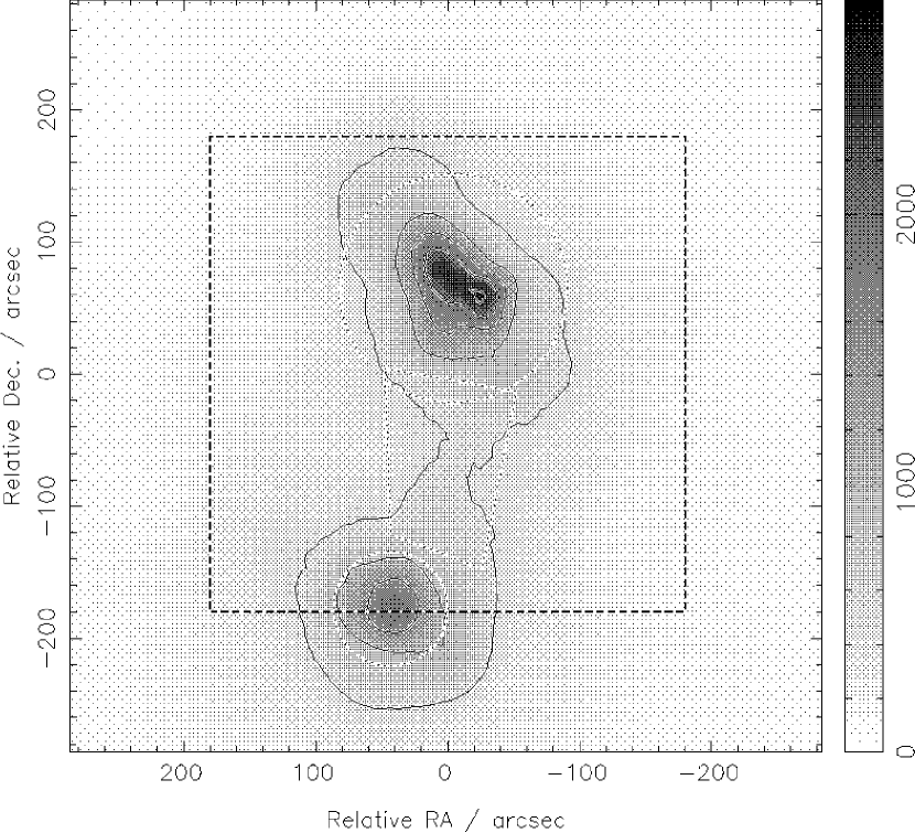
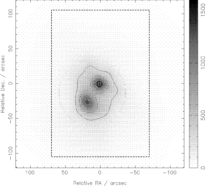
Figure 1: Projected mass distribution of two simulated clusters. Left: CL10, a massive cluster at redshift 0.2. Right: CL08, a smaller cluster at redshift 0.78. The grey scale is $\Sigma$/M_⊙ pc^-2, the contours are spaced in steps of 500 h $M_{\odot}$ pc${}^{-2})$ for CL10 and 300 h $M_{\odot}$ pc${}^{-2})$ for CL08. Also marked are the apertures used for mass estimation from the reconstructed maps (dotted) and the mock observing region (dashed).

3 Application to simulated data

To demonstrate the method outlined in the previous section we now apply it to two simulated clusters, taken from the sample generated by Eke, Navarro and Frenk [Eke et al. 1998]. The naming of the clusters is retained from that paper, in which a flat Universe dominated by a cosmological constant was assumed. The same cosmological parameters ($\Omega_{m}=0.3,\Omega_{\Lambda}=0.7$) were used to calculate the critical density and angular diameter distances needed in the lensing analysis below. The Hubble constant is taken as $100h$ km s^-1 Mpc^-1.

3.1 The mass distributions

The two projected mass distributions are shown in Figure 1. The first, CL10, is at a redshift of $0.2$, and has an X-ray emission-weighted temperature of $4.0$ keV; the second, CL08, is at redshift 0.78 with temperature $2.1$ keV. Neither cluster is extremely massive, having approximate virial masses of $6$ and $1\times 10^{14}h^{-1}M_{\odot}$ respectively. Overlaid on these plots are the observing regions corresponding approximately to the field of view of the Keck Low Resolution Imaging Spectrograph (for CL10, see e.g. Clowe et al. [Clowe et al. 2000]) and an HST mosaic comprising two WFPC2 pointings (for CL08). Also plotted are the apertures used to estimate projected masses for the cluster components. For CL10, these are circles of radius 0.2 h^-1Mpc ($\sim 87$ arcsec) and 0.1 h^-1Mpc ($\sim 43$ arcsec) centred on the large and small subclumps respectively, and are referred to as apertures 1 and 2. Aperture 3 is the quadrilateral region between the subclumps. For CL08 a single aperture is defined, being a circle of radius 0.25 h^-1Mpc ($\sim 48$ arcsec). Neither observing region is particularly large, and the smaller clump in CL10 is marginally outside the observing field. These clusters were deliberately chosen to contain ‘interesting’ substructure, in order to illustrate the angular resolution of the reconstruction method.

3.2 Simulated lensing data

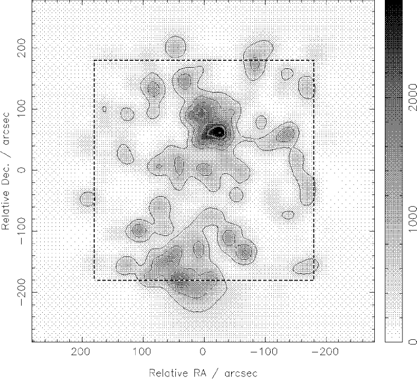
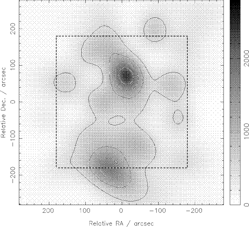
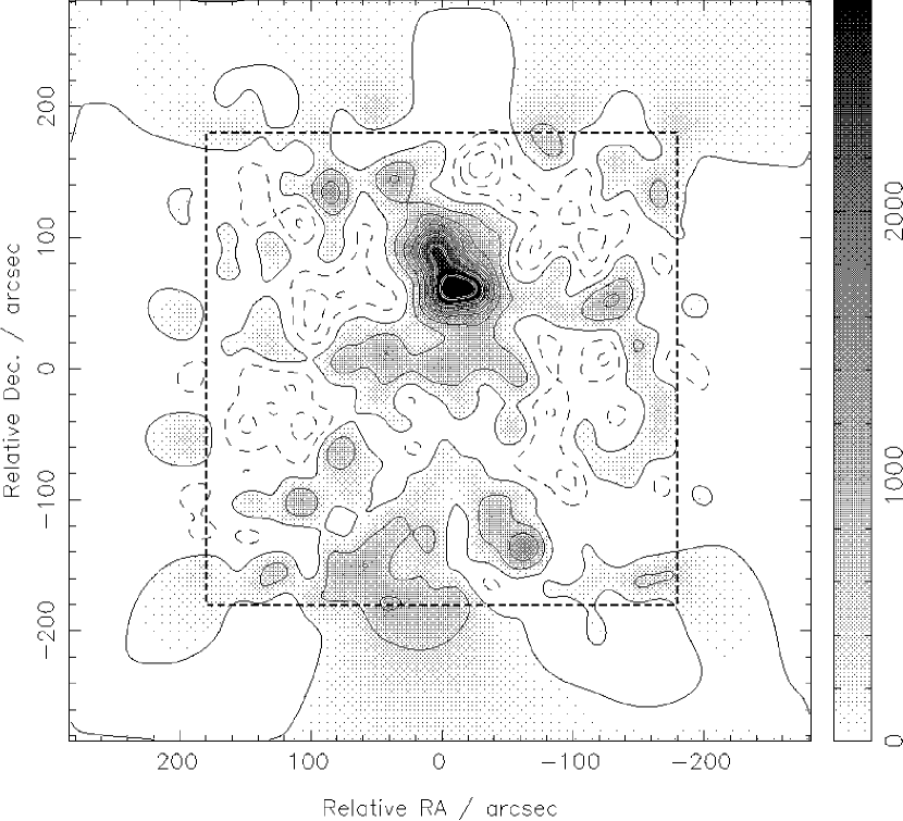
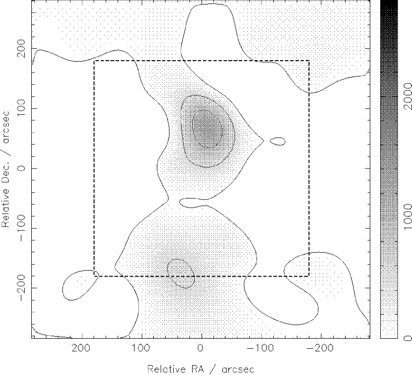
Figure 2: Top: Reconstructed mass distributions for the cluster CL10. Left to right, the ICF width parameter $w$ increases from 20 to 70 arcsec. Bottom: KS93 direct inversions for comparison; the shear data were smoothed with a Gaussian of FWHM equal to $w$ in each case. In all plots the contours show surface density in steps of 500 h $M_{\odot}$ pc^-2. The maximum on the density scale corresponds to a convergence of 0.61.

Mock galaxy ellipticity catalogues were generated using the CL10 and CL08 mass distributions as follows. The parameters of the observations described in Clowe et al. [Clowe et al. 2000] and Hoekstra et al. [Hoekstra et al. 2000] were used to estimate the background galaxy number densities obtainable in 2 hours observation with either the Keck LRIS or HST. The median galaxy redshift was estimated from the Hubble Deep Field photometric redshift catalogue [Fernandez-Soto et al. 1999], and then used to calculate an approximate value of $\Sigma_{\rm crit}$. Systematic effects due to the unknown redshift distribution of background galaxies [Fischer & Tyson 1997] are not considered here. The projected mass distributions of Figure 1 were then converted to convergence and equation (1) was applied to produce maps of the components of reduced shear $g$ on the same grid. These maps were then interpolated onto galaxy positions drawn at random from within the observing field. The components of the intrinsic ellipticity of the sources, $\epsilon^{s}_{i}$, were then drawn from a Gaussian distribution of width $\sigma_{\rm intrinisic}=0.25$ and transformed to their lensed counterparts using the relation [Seitz & Schneider 1997]

$$\epsilon=\frac{\epsilon^{s}+g}{1+g^{*}\epsilon^{s}},$$ (12)

where the asterisk denotes complex conjugation. Uncertainties introduced in the estimation of galaxy shapes were included by adding Gaussian noise with $\sigma_{obs}=0.15$. This is a reasonably pessimistic approach, with only the fainter galaxies detected having errors of this size associated with their ellipticities [Hoekstra et al. 2000, Bacon et al. 2001, Bridle et al. 2002]. The limiting magnitudes quoted should therefore be taken as those down to which image shape measurements could be made to this accuracy. The parameters of the mock observations are given in Table 1.

Table 1: Properties of the simulated 2 hour observations of section 3.

Cluster	$z$	$I_{\rm lim}$	$z_{s}$	$\Sigma_{\rm crit}$	$\kappa_{\rm peak}$	$A_{\rm obs}$	$n_{s}$	$N_{s}$
				(h $M_{\odot}\rm pc^{-2})$		($\rm arcmin^{2}$)	($\rm arcmin^{-2}$)
CL10	0.2	26.3	1.0	4634	0.61	36	40	1476
CL08	0.78	26.5	1.3	4950	0.38	8.2	100	695

From left to right: cluster name and redshift, limiting I magnitude, median source redshift, corresponding value of the critical density, cluster peak convergence, observing area, number density of background galaxies, and the total number of sources in the simulated catalogue.

3.3 Results

Reconstructions were performed for a range of Gaussian ICFs with varying FWHM $w$; the mass distributions were defined on 128 by 128 pixel grids. Each reconstruction, including aperture integrated mass estimation, required approximately two minutes of CPU time on a single R10000 processor of a Silicon Graphics Origin 200.

3.3.1 CL10

Reconstructions with ICF widths of 20 and 70 arcsec are shown in the top two panels of Figure 2. The greyscale is plotted with the same limits as used for the true mass distribution of Figure 1. For comparison, we also show results for which the mock data was first smoothed, using the same Gaussian ICFs as the smoothing kernel, and then inverted directly using the Kaiser & Squires [Kaiser & Squires 1993] algorithm to obtain a convergence map; results are plotted in the lower panel of the same figure. Here the contours are simply of the surface density, obtained by scaling the convergence by the relevant value of $\Sigma_{\rm crit}$; the greyscale is again the same as Figure 1. The grid on which the Fourier transforms were performed was padded with zeros outside the observing region to allow a more direct comparison with our method. At each smoothing scale the maps generated by the two methods contain recognisably similar structures; Figure 2 illustrates the way in which the smoothing has been moved from the data to the reconstruction. Features which differ from the true mass distribution are similar in both reconstructions, and are due to the noise realisation.

Compared to the KS93 results, the maximum-entropy solutions are preferable as they are maps of inferred physical mass (so are necessarily positive), in which the noise on each data point has been translated to inferred uncertainties in the maps. At low values of the ICF width the high noise in the shear data acts to break up the lensing signal, leading to false apparent cluster substructure at small scales. The presence of many low level spurious features is also due to this over-fitting of the data. Note that the lensing signal is not diluted by moving to higher values of $w$, in contrast to the effect of data smoothing in the KS93 process.

Figure 3: $\textrm{Pr}(w|\mbox{Data})$ for the CL10 analysis. The logarithmic scale corresponds to the joined points, while the solid bars are on the linear scale.

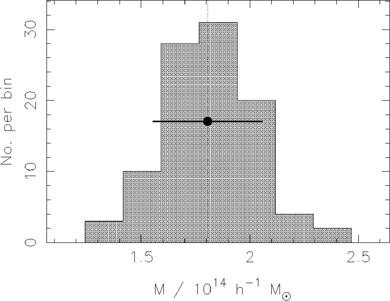
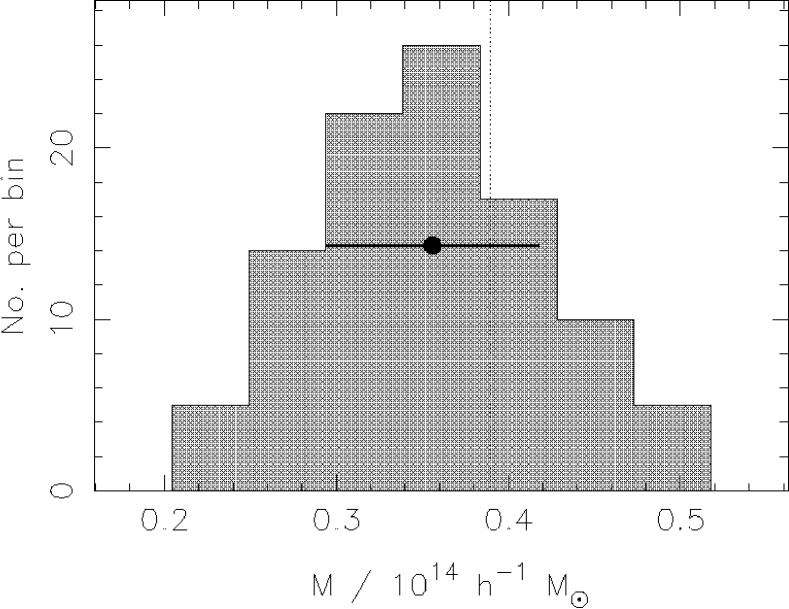
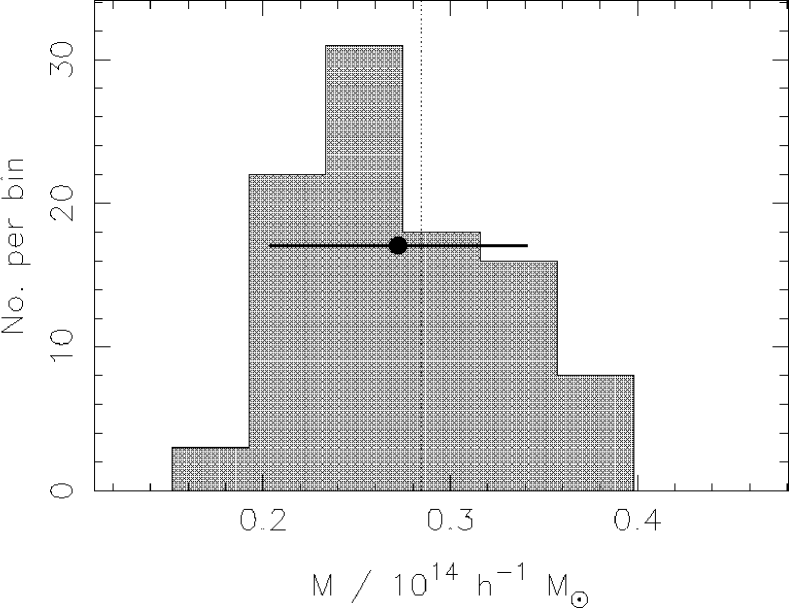
Figure 4: Mass estimates for CL10. In each panel a histogram of mass estimates from the reconstruction maps from 100 realisations of the background galaxy population are plotted. The dotted line marks the true value. The point shows the mean mass estimate; the error bar is the mean inferred error, not the standard deviation of the histogram. The apertures used are shown in Figure 1 Top: circle of radius $0.2h^{-1}$ Mpc centred on the main cluster; middle: circle of radius $0.1h^{-1}$ Mpc centred on the sub-clump; bottom: quadrilateral region between the two main mass clumps.

The two maximum-entropy reconstructions in Figure 2 are taken from the posterior probability distribution $\textrm{Pr}(w|\mbox{Data})$; as described in Section 2 this distribution is proportional to the numerically evaluated evidence and is shown in Figure 3. The shape of this graph is typical. The reduction in probability at large ICF widths is because the data are poorly fitted by the overly smooth mass distribution. At the other extreme, small ICF widths are strongly disfavoured as they effectively increase the number of free parameters in the fit; this is the ‘Occam’s razor’ factor which arises naturally from Bayesian model selection analysis (e.g., MacKay 1992) and also corresponds to the intuition that one shouldn’t over- or under-smooth data. The map corresponding to the maximum of $\textrm{Pr}(w|\mbox{Data})$ represents a ‘map of believable features’, and occurs at $w=70$ arcsec, shown in the right-hand panel of Figure 2. The contours of this reconstruction trace the two main mass condensations, and suggest the presence of a bridge of mass between them; no other significant features are visible. In the absence of further information about the cluster this map represents the most probable mass distribution, given the data and our choice of the functional form of the ICF. The eye is very sensitive to the high resolution detail of the main peak in Figure 2; however, the evidence is sensitive to the entire mass distribution, which is smooth on larger angular scales.

The projected mass within each of the three apertures shown in Figure 1 was calculated for the preferred 70 arcsec ICF width. This process was carried out on reconstructions from 100 galaxy catalogues with the same observational parameters as in Table 1 but with different galaxy positions and ellipticities. The results are shown in the histograms of Figure 4, with statistics from these measurements given in Table 2. The distributions are satisfyingly symmetrical about the true values; their widths are in very good agreement with the mean of the individual 1-sigma errors calculated from equation (10), shown by the solid error bars. This demonstrates that the noise present in the galaxy shape data has been successfully carried through to the inferred quantities.

We note that if there is no error due to the estimation of the galaxy shapes (i.e. $\sigma_{\rm obs}=0$) then the error bar on the mean inferred mass is reduced by approximately ten per cent, which corresponds roughly to the change in the combined ellipticity error $\sigma$.

Table 2: Mass estimates for CL10.

Aperture	$M_{\rm true}$	$\langle M\rangle_{100}$	$\langle\sigma_{M}\rangle_{100}$
1	1.18	$(1.18\pm 0.12)$	0.12
2	0.39	$(0.36\pm 0.07)$	0.06
3	0.28	$(0.27\pm 0.06)$	0.07
	0.12	$(0.14\pm 0.06)$	0.07

All masses are in units of $10^{14}h^{-1}$ M_⊙. Left to right, the columns contain: aperture number (see text), true projected mass within aperture, the mean and standard deviation of masses estimated from 70 arcsec reconstructions from 100 noise realisations of the dataset, and the mean inferred error of these 100 mass estimates. The final row contains mass estimation results for the third aperture translated to a region containing apparently very little mass.

We can take this analysis one step further and calculate a mass profile around the larger sub-clump; this is shown in Figure 5. The mass estimates can be seen to be accurate over a reasonable range of angular scales, with slight overestimation as the apertures extend further outside the observing region.

Figure 5: Mass profile for the largest sub-clump of cluster CL10. The points shows the mean estimated mass within that radius while the error bar is the inferred 1-sigma error (averaged over 100 noise realisations). The shaded area shows the 1-sigma dispersion in the mass estimates over the 100 realisations. The dotted line marks the true profile. $0.4h^{-1}$ Mpc corresponds to 170 arcsec.

Our analysis has at no point attempted to account for the ‘mass sheet degeneracy’ [Falco et al. 1985, Schneider & Seitz 1995]. If the observing field is sufficiently large then the entropic prior acts to pin down the reconstruction at the edge of this region (Paper II), constraining any mass sheet transformation to be small. This control of the mass sheet degeneracy is the outcome of our choice of a low default model value to be used in the cross-entropy function (see Paper II). The value used in all reconstructions in this work was 100 h $M_{\odot}$pc^-2; a lower value was found to leave the reconstruction maps and mass estimates unaffected. However, significantly increased model values gave masses overestimated by some tens of per cent, with mass sheets visibly present in the reconstructions. With the default model set suitably low, the residual effect of the mass sheet degeneracy on the mass estimates in any given reconstruction is small compared to the uncertainties due to the noise realisation; this can be seen by comparing the widths of the histograms to the ensemble-averaged error bars in Figure 4.

Interestingly, the higher resolution maps give mass estimates which are systematically below the true values: such maps provide closer fits to the noise in the data, which breaks up the coherent lensing signal leading to an underestimate of the total mass present. This also illustrates the way in which the value of $w$ preferred by the evidence is determined by the fit across the whole image, not just at the peaks of the mass distribution.

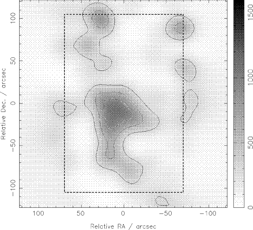
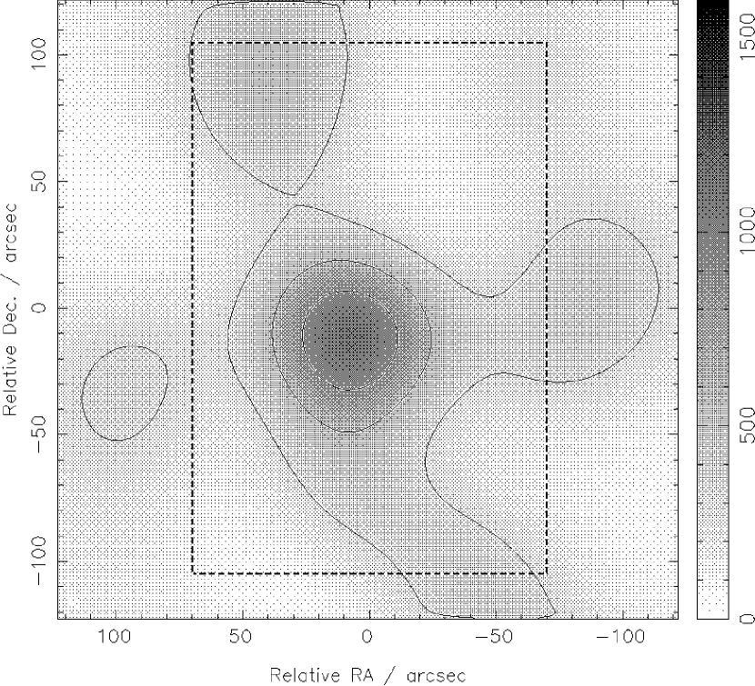
Figure 6: Top: Reconstructed mass distributions for the cluster CL08. Left to right, the ICF width parameter $w$ increases from 20 to 50 arcsec. Contours show surface density in steps of 300 h $M_{\odot}$ pc${}^{-2})$.The maximum on the density scale corresponds to a convergence of 0.38.

Although our mass estimation procedure is simplistic, it does produce sensible and accurate results, even for mass condensations located on the edges of the observing region. The filament-like structure lying between the subclumps of CL10, which was hinted at in the reconstruction maps of Figure 2, was successfully detected in that region; its mass was measured with an uncertainty of $\sim 20$ per cent. The same aperture was translated to the North-East by approximately 200 arcsec, to a region containing just $0.12\times 10^{14}h^{-1}$ M_⊙. When the mass estimation analysis was repeated, this value was also recovered to within the mean inferred error of $\sim 40$ per cent.

3.3.2 CL08

With a smaller dataset and lower peak convergence, this simulation presents a more difficult problem. The most probable Gaussian ICF width is found to be 50 arcsec and the corresponding reconstruction is shown in Figure 6. The substructure in the cluster has been smoothed over, and the peak density is underestimated by a factor of two. Although a higher resolution reconstruction, which is also shown in Figure 6, does suggest substructure, this particular noise realisation does not enable the fine detail of the true cluster mass distribution to be faithfully recovered. As an illustration, 20 arcsec ICF reconstructions of four different noise realisations are shown in Figure 7. These reconstructions were deliberately selected (from a larger sample of 20) to highlight the extremes of good and bad fortune. The presence of density peaks in the reconstructions is clearly sensitive to the particular noise realisation. In contrast, the 50 arcsec reconstructions of the noise realisations of Figure 7 are all very similar. In practice, there is only ever one available data set; for the set analysed in Figure 6 there is very little information about the two density peaks, but there is a lensing signal from the broader underlying mass distribution. The 50 arcsec reconstruction is the most probable given the data: all of the data are used to infer the global noise properties, which are then reflected in the smooth reconstruction. Given such data we can say only that cluster CL08 is extended in the North-South direction, and that there is a slight suggestion of substructure.

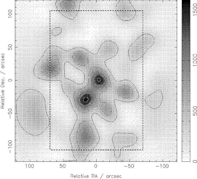
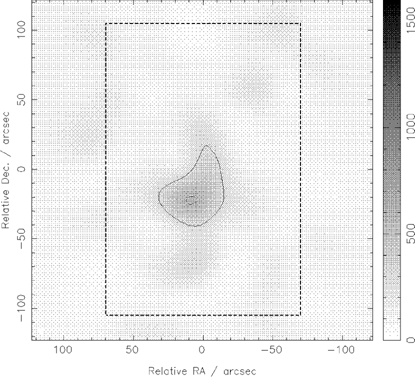
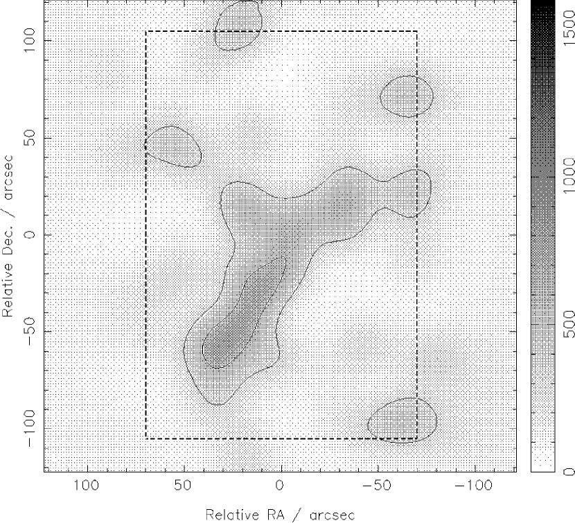
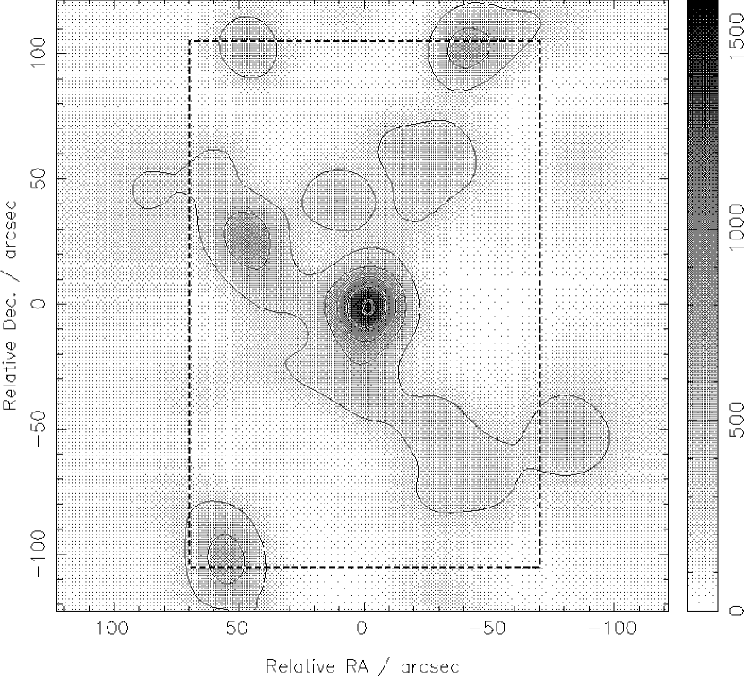
Figure 7: High resolution ($w=20$ arcsec) reconstructions of CL08, from 4 different realisations of the background galaxy population.

Despite the apparent poor quality reconstruction, the shear data are still sensitive to the total mass within an aperture: the mass estimation histogram of Figure 8 shows the total projected mass within 0.25 h^-1Mpc of the cluster centre to be well constrained by the data, with the large error bars (on average $0.2\times 10^{14}h^{-1}$ M_⊙) comparing reasonably well with the width of the histogram ($0.3\times 10^{14}h^{-1}$ M_⊙). This discrepancy reflects the larger impact of the residual mass sheet degeneracy when smaller observing fields are used. There is a tendency towards overestimation of the total mass as the additive noise in the reconstruction becomes important for this less massive cluster, but this effect is within the estimated error for the aperture considered (mean=0.92, truth=$0.74\times 10^{14}h^{-1}$ M_⊙). The effect can be seen more clearly in Figure 9 the corresponding figure to Figure 5. Note that the edge of the observing region is at $0.3h^{-1}$Mpc; in such low signal, high noise, small observations, extrapolation beyond the immediate vicinity of the cluster is clearly to be done with care. One issue is that of the prior on the ICF width – as the ICF width approaches the size of the observation the effect of the mass sheet degeneracy will increase.

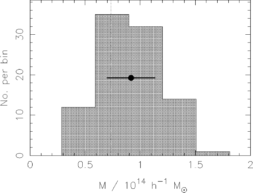
Figure 8: Mass estimates from 50 arcsec reconstructions of CL08 (see Figure 4. The aperture, shown in Figure 1 is a circle of radius $0.25h^{-1}Mpc$.

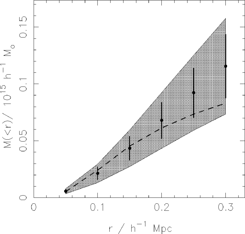
Figure 9: Mass profile for CL08. The points shows the mean estimated mass within that radius while the error bar is the inferred 1-sigma error (averaged over 100 noise realisations). The shaded area shows the 1-sigma dispersion in the mass estimates over the 100 realisations. The dotted line marks the true profile. $0.4h^{-1}$ Mpc corresponds to 80 arcsec.

3.4 More advanced analyses

The above analysis used a circularly symmetric Gaussian intrinsic correlation function, but there is no a priori reason why this smoothing kernel should give the best results. We also experimented with circular top-hat, exponential and softened isothermal (‘beta’) profiles, and all were found to give significantly lower values of the evidence for a given data set than the Gaussian ICF. The softened isothermal profile, aiming to optimise the fit to the cluster profile, was found to be worse at suppressing the noise in the outer regions of the cluster, while the presence of such broad wings introduced a large systematic overestimation of the mass integrals due to the mass sheet degeneracy. It is quite possible that the optimal ICF for the weak lensing reconstruction problem is not Gaussian, but our experience with these three alternative functions leads us to expect that any gain in evidence would be marginal, and the reconstruction for a given ICF width would be changed very little.

The argument given above against using the isothermal profile for an ICF suggests the use of more than one ICF at a time, allowing multiple resolution scales in the reconstruction. The reconstruction then consists of a weighted sum of convolutions of hidden images with varying width ICFs. This ‘multi-scale maximum-entropy’ method has been applied to a number of problems [Weir 1992, Bontekoe et al. 1994, McLachlan et al. 2002]; it allows high spatial resolution where the data warrant it. However, when multi-scale ICFs were applied to the weak lensing problems shown here, very little increase in evidence was found over the single ICF reconstructions, and the inferred mass distributions from the two approaches were indistinguishable. The introduction of another hidden image increases the size of the hypothesis space, introducing extra complexity to the reconstruction which is not justified by the quality of the data.

4 Application to real data

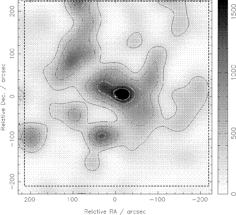
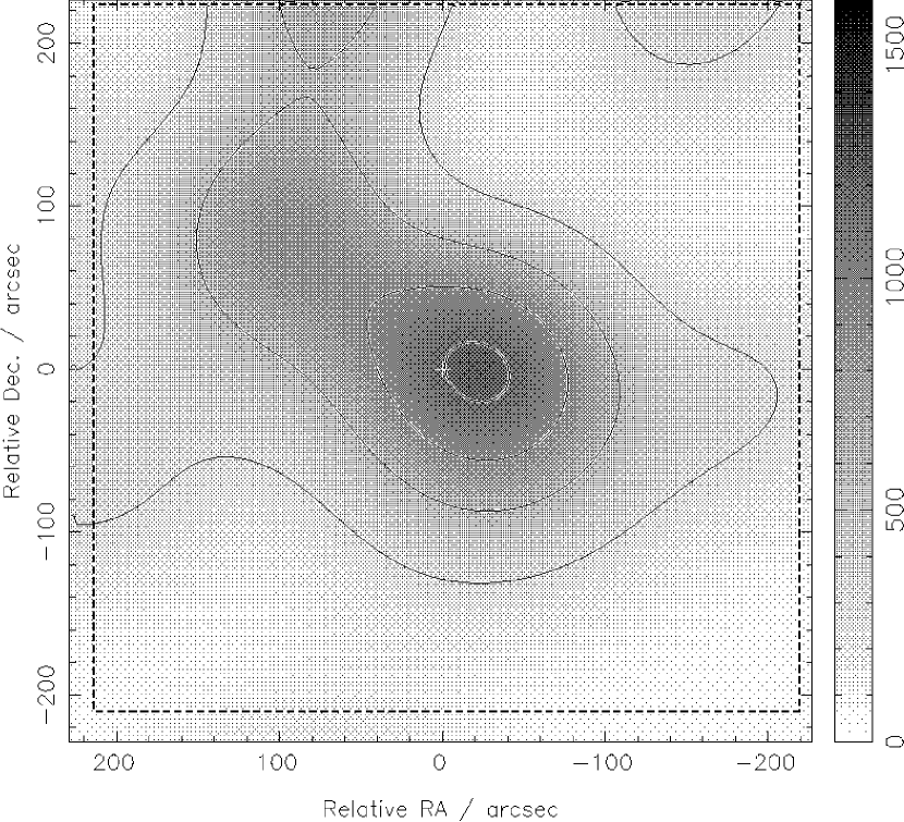
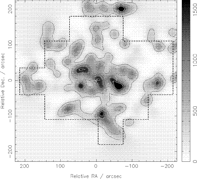
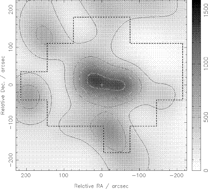
Figure 10: Top: Reconstructed mass distributions for the cluster MS1054-03. Top: 40 arcsec (left) and 120 arcsec (right) ICF width reconstructions from the Keck data of Clowe et al. Bottom: 20 arcsec (left) and 80 arcsec (right) ICF width reconstructions from the HST data of Hoekstra et al. The left-hand panels contain maps with angular resolution corresponding to that of the maps already published; the right-hand panels show the maximum evidence reconstructions. Contours show surface density in steps of 300 h $M_{\odot}$ pc^-2. The maps are centred on the brightest cluster galaxy (BCG) position, marked with a cross.

We now apply our maximum-entropy method to real data. MS1054-03 is a high redshift ($z=0.83$) galaxy cluster; X-ray and dynamical measurements suggest that it has a high mass ($T_{X}\approx 10\rm keV$, Jeltema et al. 2001, $\sigma\approx 1150$ km s^-1, van Dokkum 1999). Two sets of weak lensing data have been analysed. Clowe et al. [Clowe et al. 2000] produced a catalogue of 2723 background galaxies from a single Keck LRIS pointing, with a number density of approximately 50-60 galaxies per square arcminute. They performed a KS93 inversion using a smoothing kernel with a FWHM of approximately 40 arcsec, and found the cluster to be extended in the East-West direction; with a smaller smoothing kernel they find three mass peaks to lower significance. Hoekstra et al. [Hoekstra et al. 2000] measured the ellipticities of 2446 galaxy images from a deep HST mosaic consisting of 6 interlaced WFPC2 fields. They achieved a source density of around 80 arcmin². They used the maximum probability extension to the KS93 algorithm [Squires & Kaiser 1996] to produce a higher resolution map (smoothed with a 20 arcsec kernel) showing three distinct mass peaks.

The maximum entropy reconstructions from these data sets are shown in Figure 10 for two ICF widths, a low value of $w$ equal to that used in the previously published analysis, and the width that maximises $\textrm{Pr}(w|\mbox{Data})$. All reconstructions were performed using the Gaussian ICF on a $128\times 128$ pixel grid. Hoekstra et al. calculate observational uncertainties on their estimated galaxy shape parameters and add them in quadrature to the intrinsic dispersion; we did the same. No corresponding weighting of galaxies is present in the Keck dataset.

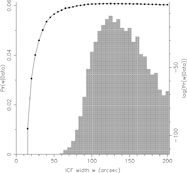
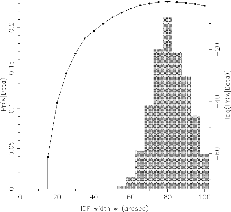
Figure 11: $\textrm{Pr}(w|\mbox{Data})$ for the MS1054-03 analyses. Top: Keck data; bottom: HST data.

Both of the high resolution maps are qualitatively very similar to those given in the referenced papers (where the data were smoothed with Gaussian kernels of the same width as the chosen low $w$ ICFs), but are now positivity-constrained. In particular, the three peaks found by Hoekstra et al. [Hoekstra et al. 2000] are reproduced along with several other features present towards the edges of their map. The reconstruction from the Keck is also similar to the one found by Clowe et al. [Clowe et al. 2000].

We now consider the probability distribution of the ICF width parameter $w$. This is shown for the two datasets in Figure 11. In both cases the evidence peaks at a significantly larger value of $w$ than that used in the high resolution maps. These ‘maps of believable features’ clearly show the absence of significant structure away from the central cluster region, and suggest that the quality of the data is such that the substructure observed in the high resolution maps of Figure 10 should be interpreted with caution. A measure of the goodness-of-fit of the two different resolution maps to the data was obtained by calculating the chi-squared statistic of equation 3, with the summation now running over the galaxies contained within 40 arcsec radii apertures placed over the three candidate sub-clumps inferred from the HST data. Reduced chi-squared values were calculated by dividing by the number of galaxies in the aperture ($\approx 280$) minus the number of pixels in the aperture ($\approx 100$); these are given in table 3.

Table 3: Reduced chi-squared values for each of the three candidate sub-clumps in MS1054-03.

Sub-clump	$\chi^{2}_{20}$	$\chi^{2}_{80}$
West	1.18	1.20
Centre	1.09	1.10
East	1.20	1.26

The subscripts refer to the resolution scale $w$ of the reconstruction. Note that in each case the half-width of the reduced chi-squared distribution is approximately $\sqrt{2\times 180}/180=0.1$.

It can be seen from this table that there is only a marginal improvement in the fit to the data by decreasing the ICF width; this improvement is heavily outweighed by the “Occam’s razor” factor present in the Bayesian evidence, which suggests that the extra complexity in the inferred mass distribution introduced by using an ICF width of less than 80 arcsec is not justified by these data alone.

The two datasets are by no means independent noise realisations, since they are both observations of the same background galaxy population. However, the different observing conditions have clearly introduced different galaxy shape measurement errors. The resulting difference in the details of the high resolution maps of Figure 10 apparently accords with the conclusions drawn from the probability distribution of the resolution parameter $w$. However the differences will also partly be due to the different weighting of the images in the two datasets.

As stated before, in the absence of any other information about the cluster the maximum evidence map represents the most probable mass distribution given the data; the additional information present in the cluster galaxy light and number density distributions [Hoekstra et al. 2000], and the X-ray surface brightness maps [Donahue et al. 1998, Jeltema et al. 2001] are clearly very important in the detailed interpretation of the weak lensing data, and ideally should be included in a joint analysis.

The projected mass within $0.5h^{-1}$ Mpc (94 arcsec in the cosmology of Section 3) of the brightest cluster galaxy was calculated using the method outlined in Section 2. This was done for both maps given in the lower panels of Figure 10, and the results compared with that from Hoekstra et al. [Hoekstra et al. 2000] in Table 4. Both the high and the low resolution mass estimates are consistent with the mass derived, from the tangential shear in circular apertures about the brightest cluster galaxy, by Hoekstra et al. It is reassuring to note that the statistical errors on these mass estimates agree very well with those calculated by aperture mass densitometry elsewhere. The issue of which resolution reconstruction, and so which mass estimate, to prefer may depend on prejudices about the likely level of substructure in this cluster. Given no other information about MS1054-03 we would conclude that the quality of the data suggest the 70 arcsec resolution map as being the more probable, but that there is strong evidence for substructure in the core of this cluster; in any case the weak lensing data give a projected mass of $10^{15}h^{-1}$ M_⊙ with a statistical error of about 10 per cent.

Table 4: Mass estimates for MS1054-03.

Reconstruction:	$M/10^{15}h^{-1}$ M⊙
$w=20$	$(0.91\pm 0.09)$
$w=80$	$(1.21\pm 0.15)$
Hoekstra et al. 2000	$(1.07\pm 0.12)$

All masses refer to the projected mass within $0.5h^{-1}$ Mpc of the BCG (located at the origin) and are in units of $10^{15}h^{-1}$ M_⊙. Only the HST data is used here, to allow direct comparison with Hoekstra et al.

5 Conclusions

We have developed a Bayesian analysis, based on the maximum-entropy method of Bridle et al. (1998, 2001), for inferring the distribution of mass in clusters of galaxies from weak lensing shear data. We treat each background galaxy image as a noisy estimator of the reduced shear field of the cluster, retaining all the information about both signal and noise and so allowing the for high angular resolution. Use of an ‘intrinsic correlation function’ in the maximum-entropy formalism provides a way of incorporating our prior expectation of clusters as smooth, extended objects, and effectively replaces the data smoothing required by direct reconstruction methods. In contrast to the these methods, the lensing signal is not diluted by this process. Moreover, analysis of the posterior probability distribution of the ICF width $w$, obtained by numerically evaluating the Bayesian evidence, provides an objective way of discriminating between smoothing scales. The map at the peak of this probability distribution was found not to contain any significant spurious peaks, and can be interpreted as the safest conclusion to draw from the data. The higher resolution maps, although representing an overfit to the data, do contain limited useful information particularly with respect to substructure in the cluster; the fact that their angular resolution is less favoured by the data quality gives a useful indication of the believability of these features.

Simple mass estimates extracted directly from the mass maps preferred by the evidence were found to be unbiased and accurate to within the estimated errors over a fairly wide range of angular scales; these uncertainties agreed very well with the standard deviation in the mass estimates from 100 different realisations of the background galaxy population. Noisier observations over a smaller field of view were found to give mass estimates with a slight bias towards overestimation, an effect understood in terms of the additivity of the reconstructed distribution and the mass sheet degeneracy. Inspection of the variety of structure in reconstructions from these different noise realisations justified the cautious interpretation of the high resolution maps, indicating that this analysis provides a useful way of understanding the noise properties of the data.

We have applied our method to two galaxy shape datasets for the high redshift cluster MS1054-03, one derived from a ground based observation and the other from an HST mosaic. In both cases the features found in previously published maps, obtained by both direct and inverse methods, are reproduced, but with the added desirable features of being positivity-constrained and quantitatively useful. Simple mass estimates extracted directly from the reconstruction agree well with values found by aperture mass densitometry, as do the errors estimated by both methods.

The principal function of parameter-free mass maps as produced by this method is to provide the equivalent of a mass telescope, allowing images to be generated to aid further, more quantitative analysis. Parameterised fitting to shear data with physical motivation has been performed elsewhere [Schneider et al. 2000, King & Schneider 2001]; we believe that the information provided by our variable angular resolution analysis is a helpful guide to this process, whilst also providing reasonably accurate ‘mass photometry’ at the same time. The use of the Bayesian evidence in such fitting will be addressed in future papers.

Acknowledgments

We thank Henk Hoekstra and Douglas Clowe and their co-workers for supplying us with their data, and Vincent Eke for providing the simulated projected mass distributions.

Thanks are also due to Andy Taylor, Richard Saunders and Charles McLachlan for helpful discussions, and to Anton Garret for proof-reading the manuscript. We also thank the anonymous referee for comments leading to improvements in the paper.

PJM acknowledges the PPARC for support in the form of a Research Studentship. The MEMSYS4 code was developed by Maximum Entropy Data Consultants Ltd., and is available for use by the astronomical community under the name ‘LensEnt2’. This can be obtained from http://www.mrao.cam.ac.uk/projects/lensent/

References

- [Bacon et al. 2001] Bacon D.J. Refregier A., Clowe D., Ellis R.S., 2001, MNRAS, 325, 1065
- [Bartelmann 1995] Bartelmann M., 1995, A&A, 303, 643
- [Bartelmann et al. 1996] Bartelmann M., Narayan R., Seitz S., Schneider P., 1996, ApJ, 464, L115
- [Bontekoe et al. 1994] Bontekoe Tj.R., Koper E., Kester D.J.M., 1994, A&A, 284, 1037
- [Bridle et al. 1998] Bridle S.L., Hobson M.P., Lasenby A.N., Saunders R.D.E., 1998, MNRAS, 299, 895, Paper I
- [Bridle et al. 2001] Bridle S.L., Hobson M.P., Marshall P.J., Saunders R.D.E., Lasenby A.N., 2001, MNRAS submitted (astro-ph/0010387), Paper II
- [Bridle et al. 2002] Bridle S.L. et al. , 2002, in preparation
- [Broadhurst et al. 2001] Broadhurst T., Taylor A., Peacock J., 1995, ApJ, 438, 49
- [Clowe et al. 2000] Clowe D., Luppino G.A., Kaiser N., Gioia I., 2000, ApJ, 539, 540
- [van Dokkum 1999] P. van Dokkum (1999), PhD. thesis, University of Groningen.
- [Donahue et al. 1998] Donahue M., Voit G.M., Gioia I., Luppino G.A., Hughes J.P., Stocke J.T., 1998, ApJ, 502, 550
- [Dye & Taylor 1998] Dye S., Taylor A., 1998, MNRAS, 300, L23
- [Eke et al. 1998] Eke V.R., Navarro J.F., Frenk C.S., 1998, ApJ, 503, 569
- [Erben et al. 2000] Erben Th., van Waerbeke L., Mellier Y., Schneider P., Cuillandre J-C., Castander F.J., Dantel-Fort M., 2000, A&A, 355, 23
- [Falco et al. 1985] Falco E.E., Gorenstein M.V., Shapiro I.I., 1985, ApJ, 289, L1
- [Fernandez-Soto et al. 1999] Fernandez-Soto A., Lanzetta K.M., Yahil A., 1999, ApJ, 513, 34
- [Fischer & Tyson 1997] Fischer P., Tyson J.A., 1997, AJ, 114, 1
- [Gull 1989] Gull S. F., 1989, in Skilling J., ed., Maximum Entropy and Bayesian Methods. Kluwer, Dordrecht, p. 53
- [Gull 1990] Gull S.F., Skilling J., 1990, The MEMSYS5 Users’ Manual. Maximum Entropy Data Consultants Ltd, document available from www.maxent.co.uk
- [Hoekstra et al. 2000] Hoekstra H., Franx M., Kuijken K., 2000, ApJ, 532, 88
- [Hoekstra et al. 2001] Hoekstra H., Franx M., Kuijken K., van Dokkum P.G., 2001, MNRAS submitted (astro-ph/0109445)
- [Jeltema et al. 2001] Jeltema T., Canizares C.R., Bautz M.W., Malm M.R., Donahue M., Garmire G.P., 2001, ApJ submitted (astro-ph/0107314)
- [Kaiser 1995] Kaiser N., 1995, ApJ, 439, L1
- [Kaiser & Squires 1993] Kaiser N., Squires G., 1993, ApJ, 404, 441, KS93
- [Kaiser et al. 1995] Kaiser N., Squires G., Broadhurst T., 1995, ApJ, 449, 460
- [King & Schneider 2001] King L.J., Schneider P., 2001, A&A, 369, 1
- [Kneib et al. 1994] Kneib J.-P., Mathez G., Fort B., Mellier Y., Soucail G., Longaretti P.-Y., 1994, A&A, 286, 701
- [MacKay 1992] MacKay D.J.C., 1992, Neural Computation, 4, 415
- [McLachlan et al. 2002] McLachlan C.I., Hobson M.P., Gull S.F., 2002, in preparation
- [Robinson 1992] Robinson D., 1992, PhD. thesis, University of Cambridge.
- [Schneider & Seitz 1995] Schneider P., Seitz C., 1995, A&A, 294, 411
- [Schneider et al. 2000] Schneider P., King L., Erben Th., 2000, A&A, 353, 41
- [Schramm & Kayser 1995] Schramm T., Kayser R., 1995, A&A, 289, L5
- [Seitz & Schneider 1995] Seitz C., Schneider P., 1995, A&A, 297, 287
- [Seitz & Schneider 1996] Seitz S., Schneider P., 1996, A&A, 305, 383
- [Seitz & Schneider 1997] Seitz C., Schneider P., 1997, A&A, 318, 687
- [Seitz et al. 1998] Seitz S., Schneider P., Bartelmann M., 1998, A&A, 337, 325
- [Sivia 1996] Sivia D.S., 1996, Data Analysis – A Bayesian Tutorial. OUP, Oxford.
- [Skilling 1989] Skilling J., 1989, in Skilling J., ed., Maximum Entropy and Bayesian Methods. Kluwer, Dordrecht, p. 45
- [Squires & Kaiser 1996] Squires G., Kaiser N., 1996, ApJ, 473, 65
- [Smail et al. 1995] Smail I., Hogg D. W., Yan L., Cohen J. G., 1995 ApJ, 449, L105
- [Tyson et al. 1990] Tyson J.A., Valdes F., Wenk R.A., 1990, ApJ, 349, L1
- [van Waerbeke 2000] van Waerbeke L., 2000, MNRAS, 313, 524
- [Weir 1992] Weir N., 1992, in “Astronomical Data Analysis Software and Systems I”, eds. Worrall D.M., Biemesderfer C., Barnes J., ASP Conf. Series vol. 25 186