CMB Polarization: Scientific Case and Data Analysis Issues

Abstract

We review the science case for studying CMB polarization. We then discuss the main issues related to the analysis of forth-coming polarized CMB data, such as those expected from balloon-borne (e.g. BOOMERanG) and satellite (e.g. Planck) experiments.

1 Introduction

Strong theoretical arguments suggest the presence of fluctuations in the polarized component of the cosmic microwave background (CMB) at a level of 5-10% of the temperature anisotropy. A wealth of scientific information is expected to be encoded in this polarized signal. However, while the existence of anisotropies in the temperature of the Cosmic Microwave Background (CMB) has now been firmly established by several experiments boom ; max ; dasi , only upper limits are currently available for fluctuations in the polarization of the CMB radiation.

The prospect of detecting CMB polarization anisotropy at small angular scales is now more promising than in the past. In the next few years, a number of experiments (e.g. BOOMERanG, Planck) will have the right sensitivity, as well as the necessary control on systematic effects, to make the measurement of polarization an achievable goal.

In this contribution we will first quickly review the major features of CMB polarization, then we will address some of the issues that will have to be faced in order to analyze the data collected by the forthcoming experiments.

2 CMB Polarization: Theoretical Framework

There are at least three features of CMB polarization that make it an appealing target for observation. First, CMB polarization anisotropies are generated at last scattering, so they are not affected by effects taking place after recombination, as opposed to temperature anisotropies. Second, distinctive polarization patterns are produced by different kind of density perturbations (e.g. scalar, vector, tensor). Finally polarization provides information complementary to temperature, helping in clarifying issues such as cosmological parameter degeneracies in the temperature power spectrum.

The rest of this chapter covers basic theoretical aspects of CMB polarization. Excellent reviews on the subject are koso ; primer .

2.1 Formalism

A useful way to characterize the polarization properties of the CMB is to use the Stokes parameters formalism chandra . For a nearly monochromatic plane electromagnetic wave propagating in the $z$ direction,

$$E_{x}=a_{x}(t)\cos\left[\omega_{0}t-\theta_{x}(t)\right],\ \ \ \ \ \ E_{y}=a_{y}(t)\cos\left[\omega_{0}t-\theta_{y}(t)\right],$$ (1)

the Stokes parameters are defined by:

$$I\equiv\langle a_{x}^{2}\rangle+\langle a_{y}^{2}\rangle,\ \ \ \ \ \ \ \ Q\equiv\langle a_{x}^{2}\rangle-\langle a_{y}^{2}\rangle,\ \ \ \ \ \ \ \ U\equiv\langle 2a_{x}a_{y}\cos(\theta_{x}-\theta_{y})\rangle,\ \ \ \ \ \ \ \ V\equiv\langle 2a_{x}a_{y}\sin(\theta_{x}-\theta_{y})\rangle,$$ (2)

where the brackets $\langle\rangle$ represent time averages. The parameter $I$ is simply the average intensity of the radiation. The polarization properties are described by the remaining parameters: $Q$ and $U$ describe linear polarization, while $V$ describes circular polarization. Unpolarized radiation (or natural light) is characterized by having $Q=U=V=0$. CMB polarization is produced through Thomson scattering (see below) which, by symmetry, cannot generate circular polarization. Then, $V=0$ always for CMB polarization. The Stokes parameters $Q$ and $U$ are not scalar quantities. If we rotate the reference frame of an angle $\phi$ around the direction of observation, $Q$ and $U$ transform as:

$$Q^{\prime}=Q\cos(2\phi)+U\sin(2\phi),\ \ \ \ \ \ U^{\prime}=-Q\sin(2\phi)+U\cos(2\phi).$$ (3)

We can define a polarization vector ${\bf P}$ having:

$$\left|{\bf P}\right|=\left(Q^{2}+U^{2}\right)^{1/2},\ \ \ \ \ \alpha={1\over 2}\tan^{-1}\left({U\over Q}\right).$$ (4)

Although ${\bf P}$ is a good way to visualize polarization, it is not properly a vector, since it remains identical after a rotation of $\pi$ around $z$, thus defining an orientation but not a direction. Mathematically, $Q$ and $U$ can be thought as the components of the second-rank symmetric trace-free tensor:

$${\bf P}_{ab}={1\over 2}\left(\begin{array}[]{cc}Q&-U\sin\theta\\ \vskip 6.0pt\cr-U\sin\theta&-Q\sin^{2}\theta\\ \end{array}\right),$$ (5)

where the trigonometric functions come from having adopted a spherical coordinate system.

2.2 Physical Mechanisms

The CMB photons interact before recombination with the free electrons of the primeval plasma through Thomson scattering. The dependence of the Thomson scattering cross-section on polarization is given by:

$${d\sigma\over d\Omega}={3\sigma_{T}\over 8\pi}\left|\hat{\epsilon}\cdot\hat{\epsilon}^{\prime}\right|^{2},$$ (6)

where $\hat{\epsilon}$ and $\hat{\epsilon}^{\prime}$ are incident and scattered polarization directions. After scattering, initially unpolarized light has:

$$I={3\sigma_{T}\over 16\pi}I^{\prime}\left(1+\cos^{2}\theta\right),\ \ \ \ \ \ Q={3\sigma_{T}\over 16\pi}I^{\prime}\sin^{2}\theta,\ \ \ \ \ \ U=0.$$ (7)

Integrating over all incoming directions gives:

$$I={3\sigma_{T}\over 16\pi}\left[{8\over 3}\sqrt{\pi}\,a_{00}+{4\over 3}\sqrt{\pi\over 5}a_{20}\right],\ \ \ \ \ \ Q-iU={3\sigma_{T}\over 4\pi}\sqrt{2\pi\over 15}a_{22}.$$ (8)

Then, polarization is only generated when a quadrupolar anisotropy in the incident light at last scattering is present. This has two important consequences. Because it is generated by a causal process, CMB polarization peaks at scales smaller than the horizon at last scattering. Moreover, the degree of polarization depends on the thickness of last scattering surface. As a result, the polarized signal for standard models at angular scales of tens of arcminutes is about $10\%$ of the total intensity (even less at larger scales). Typically, this means a polarized signal of a few $\mu$K.

2.3 Statistics

Since polarization is not a scalar, it cannot be expanded over the sky using spherical harmonics, as it is done with temperature. We can however expand the polarization tensor using the tensor spherical harmonics basis varsha , as:

$${\bf P}_{ab}=T_{0}\sum_{l=2}^{\infty}\sum_{m=-l}^{l}\left[a_{(lm)}^{\rm E}Y_{(lm)ab}^{\rm E}+a_{(lm)}^{\rm B}Y_{(lm)ab}^{\rm B}\right]$$ (9)

where the $E$ and $B$ labels refer to the scalar and pseudo-scalar components of the polarization tensor. The statistical properties of the CMB anisotropies polarization are then characterized by six power spectra: $C_{l}^{T}$ for the temperature, $C_{l}^{E}$ for the E-type polarization, $C_{l}^{B}$ for the B-type polarization, $C_{l}^{TE}$, $C_{l}^{TB}$, $C_{l}^{EB}$ for the cross correlations. For the CMB, $C_{l}^{TB}=C_{l}^{EB}=0$. Furthermore, since $B$ relates to the component of the polarization field which possesses a handedness, one has $C_{l}^{B}=0$ for scalar density perturbations. The detection of a non zero $B$ component would point to the existence of a tensor contribution to density perturbations.

The relation relating ($E$,$B$) to ($Q$,$U$) has a non-local nature. In the limit of small angles it can be written as:

$$E(\bf{\theta})=-\int d^{2}{\bf\theta}^{\prime}\ \omega(\tilde{\theta})\ Q_{r}({\bf\theta}^{\prime}),\ \ \ \ \ \ B(\bf{\theta})=-\int d^{2}{\bf\theta}^{\prime}\ \omega(\tilde{\theta})\ U_{r}({\bf\theta}^{\prime}),$$ (10)

where the 2D angle $\bf{\theta}$ defines a direction of observation in the coordinate system perpendicular to $z$,

$$Q_{r}({\bf\theta})=Q({\bf\theta}^{\prime})\cos(2\tilde{\phi})-U({\bf\theta}^{\prime})\sin(2\tilde{\phi}),\ \ \ \ \ \ \ U_{r}({\bf\theta})=U({\bf\theta}^{\prime})\cos(2\tilde{\phi})+Q({\bf\theta}^{\prime})\sin(2\tilde{\phi}).$$ (11)

and $\omega(\tilde{\theta})$ is a generic window function.

2.4 Theoretical Predictions

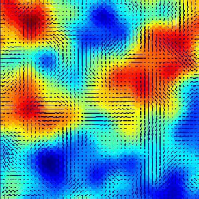
Figure 1: A simulated CMB temperature map and the corresponding polarized component represented by the polarization vector $|{\bf P}|$, for a standard cosmological model where only scalar density perturbations are present. The field is $6^{\circ}\times 6^{\circ}$, the resolution is $10^{\prime}$ FWHM.

The theoretical study of the CMB, for what concerns both its polarized and unpolarized components, is in a fully mature stage. We can produce high-precision predictions of the expected statistical CMB pattern for any given cosmological model. Figure 1 shows a simulated map of the CMB temperature anisotropy, and the corresponding polarization field, represented by the polarization vector $|{\bf P}|$. This kind of simulation can be very helpful in investigating optimal observational strategy for future experiments. In particular, now that high-resolution CMB temperature maps are available for certain areas of the sky, one can use this information to predict the statistical properties of the expected polarized signal in those regions, and tailor the polarization observations to enhance the likelihood of a detection.

Figure 2: Top panel – Temperature power spectra for a standard CDM model (solid line), and the same CDM model with a fraction of the critical density coming from a cosmological constant (dotted line). If we add to the latter a contribution from tensor perturbations (gravitational waves background) and reionization (dashed line) we can make it indistinguishable from the standard CDM model. Bottom panel – The same models and their polarization power spectra. The CDM model can be identified by its polarized signal, because it does not generate a B-type component

Figure 2 shows an example of how a polarization measurement could complement the information from temperature. Two models that would be undistinguishable from their temperature power spectra (because of the degeneracy between the effect of reionization and of tensor modes) can be discerned by their signature in the polarization power spectrum: only the model having a tensor contribution produces B-type polarization. Furthermore, reionization produces a bump at low $l$’s in the polarization spectrum.

3 CMB Polarization: Data Analysis

In order to extract the cosmological information encoded in the CMB polarization, one has to face the challenge of a complicated data analysis stage after the observations are performed. CMB data analysis was successfully performed for recent CMB temperature experiments. While analyzing polarized data is in principle not different from unpolarized data, further complications have to be addressed. In the following we show how the problem of producing polarized maps from time-ordered observations can be addressed using the same kind of algorithms and formalism developed for the temperature case natoli .

3.1 Map-making

We can write the total signal measured from a generic noiseless polarimeter as:

$$\mathcal{M}=\frac{1}{2}\left(I+Q\cos 2\phi+U\sin 2\phi\right).$$ (12)

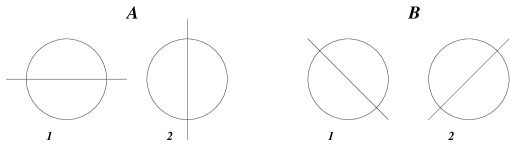
Figure 3: Experimental set-up for two radiometers, each measuring two polarization states at $90^{\circ}$ orientation. Furthermore, the radiometer B polarimeters are at $45^{\circ}$ with respect to radiometer A

Consider the experimental set-up shown in Figure 3, where the four polarimeters are assumed to observe the same point on the sky. Then, one can write:

$$Q = \left(\mathcal{M}_{A1}-\mathcal{M}_{A2}\right)\cos 2\phi-\left(\mathcal{M}_{B1}-\mathcal{M}_{B2}\right)\sin 2\phi$$ (13)

$$U = \left(\mathcal{M}_{A1}-\mathcal{M}_{A2}\right)\sin 2\phi+\left(\mathcal{M}_{B1}-\mathcal{M}_{B2}\right)\cos 2\phi.$$ (14)

More generally, the time-ordered data stream for a noisy polarimeter $(i)$ is:

$$d_{t}^{\left(i\right)}=\frac{1}{2}A_{tp}^{\left(i\right)}\left[I+Q_{p}\cos 2\phi_{t}^{\left(i\right)}+U_{p}\sin 2\phi_{t}^{\left(i\right)}\right]+n_{t}^{\left(i\right)}.$$ (15)

For the previous set-up:

$$\widetilde{d_{t}}^{A} = A_{tp}^{A}\left[Q_{p}\cos 2\psi_{t}+U_{p}\sin 2\psi_{t}\right]+\widetilde{n_{t}}^{A}$$ (16)

$$\widetilde{d_{t}}^{B} = A_{tp}^{B}\left[-Q_{p}\sin 2\psi_{t}+U_{p}\cos 2\psi_{t}\right]+\widetilde{n_{t}}^{B},$$ (17)

where:

$$\widetilde{d_{t}}^{A}\equiv d_{t}^{A1}-d_{t}^{A2},\ \ \ \ \ \ \widetilde{d_{t}}^{B}\equiv d_{t}^{B1}-d_{t}^{B2},\ \ \ \ \ \ \widetilde{n_{t}}^{A}\equiv n_{t}^{A1}-n_{t}^{A2},\ \ \ \ \ \ \widetilde{n_{t}}^{B}\equiv n_{t}^{B1}-n_{t}^{B2}.$$ (19)

We can recast everything in a matrix formalism:

$$\mathbf{D}_{t}=\mathbf{A}_{tp}\mathbf{S}_{p}+\mathbf{n},$$ (20)

where:

$$\mathbf{D}_{t}\equiv\left(\begin{array}[]{c}\widetilde{d_{t}}^{A}\\ \widetilde{d_{t}}^{B}\end{array}\right),\ \ \ \ \ \ \mathbf{A}_{tp}\equiv\left(\begin{array}[]{cc}\cos 2\psi_{t}A_{tp}^{A}&\sin 2\psi_{t}A_{tp}^{A}\\ &\\ -\sin 2\psi_{t}A_{tp}^{B}&\cos 2\psi_{t}A_{tp}^{B}\end{array}\right),\ \ \ \ \ \ \mathbf{S}_{p}\equiv\left(\begin{array}[]{c}Q_{p}\\ U_{p}\end{array}\right),\ \ \ \ \ \ \mathbf{n}_{t}\equiv\left(\begin{array}[]{c}n_{t}^{A}\\ n_{t}^{B}\end{array}\right).$$ (21)

We then obtain the standard map-making solution:

$$\mathbf{\widetilde{S}_{p}}=\left(\mathbf{A}^{t}\mathbf{N}^{-1}\mathbf{A}\right)\mathbf{A}^{t}\mathbf{N}^{-1}\mathbf{D},$$ (22)

where:

$$\mathbf{N}\equiv\left\langle\mathbf{n}_{t}\mathbf{n}_{t^{\prime}}\right\rangle=\left(\begin{array}[]{cc}\left\langle n_{t}^{A}n_{t^{\prime}}^{A}\right\rangle&\left\langle n_{t}^{A}n_{t^{\prime}}^{B}\right\rangle\\ &\\ \left\langle n_{t}^{B}n_{t^{\prime}}^{A}\right\rangle&\left\langle n_{t}^{B}n_{t^{\prime}}^{B}\right\rangle\end{array}\right),$$ (23)

which can be further simplified if:

$$\left\langle n_{t}^{A}n_{t^{\prime}}^{B}\right\rangle\ =\left\langle n_{t}^{B}n_{t^{\prime}}^{A}\right\rangle=\mathbf{0}.$$ (24)

An example of the application of this procedure is shown in Figure 4, for the 100 GHz channel of Planck Low Frequency Instrument.

4 Conclusions

Temperature anisotropy measurements have just started to have the accuracy required for high precision cosmology. Polarization has enormous scientific potential, but is still a big challenge, both experimentally (low signal, fine-scale structure, systematics, etc.) and for data analysis (which must be both accurate and efficient). The next few years will most likely bring us definitive high-resolution high-sensitivity maps of the CMB temperature anisotropy by satellites (MAP, Planck). The new frontier of cosmological exploration will then shift towards observations of CMB polarization, which will certainly provide us with new insights about the physics of the early universe.

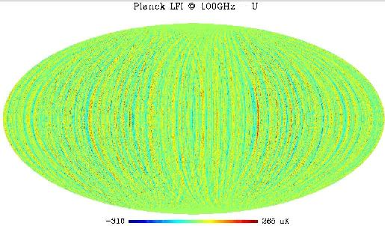
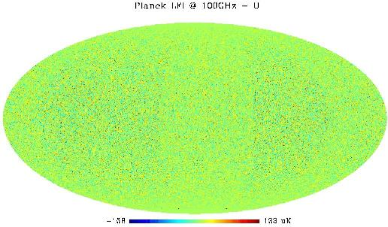
Figure 4: Simulated maps for the 100 GHz channels (32 radiometers) of Planck/LFI. Shown from top to bottom are the I, Q and U components, obtained by a naive coadding of observations in each pixel (left) and using the map-making procedure described in the text (right).

References

• (1) De Bernardis, P., et al., Nature 404 (2000) 955-959
• (2) Hanany, S., et al., Astrophys.J. 545 (2000) L5
• (3) Halverson, N.W., et al., Astrophys.J. in press (2001)
• (4) Kosowsky, A., Annals Phys. 246 (1996) 49-85
• (5) Hu, W. & White, M., New Astron. 2 (1997) 323
• (6) Chandrasekhar, S., Radiative Transfer (1960) Dover, New York
• (7) Varshalovich, D.A., Moskalev, A.N. and Khersonskii, V.K., Quantum Theory of Angular Momentum (1988) World Scientific, Singapore
• (8) Natoli, P., et al., A&A 372 (2001) 346-356