Polarization of resonance X-ray lines from clusters of galaxies

Abstract

As is known, resonant scattering can distort the surface-brightness profiles of clusters of galaxies in X-ray lines. We demonstrate that the scattered line emission should be polarized and possibly detectable with near-future X-ray polarimeters. Spectrally-resolved mapping of a galaxy cluster in polarized X-rays could provide valuable independent information on the physical conditions, in particular element abundances and the characteristic velocity of small-scale turbulent motions, in the intracluster gas. The expected degree of polarization is of the order of 10% for richest regular clusters (e.g. Coma) and clusters whose X-ray emission is dominated by a central cooling flow (e.g. Perseus or M87/Virgo).

1 Introduction

Although the intergalactic gas in clusters of galaxies is optically thin to Thomson scattering ($\tau_{\rm T}\mathrel{\hbox{\hbox to0.0pt{\hbox{\lower 4.0pt\hbox{$\sim$}}\hss}\hbox{$<$}}}0.01$) for the continuum photons, it can be moderately thick ($\tau\sim 1$) in the resonance X-ray lines of highly ionized atoms of heavy elements. This causes the radiative transfer in such lines to be important and gives rise to three major observable effects as previously discussed in the literature.

First, the surface-brightness profile of a cluster in a resonance line, calculated in the optically-thin limit, should be distorted due to diffusion of photons from the dense core into the outer regions of the cluster (Gilfanov, Sunyaev & Churazov 1987a; Shigeyama 1998). This must be taken into account when attempting to determine element abundances from X-ray spectroscopic observations of galaxy clusters or haloes of elliptical galaxies. This effect has been already considered in application to ASCA, Beppo-SAX and XMM-Newton data [Akimoto et al. 1997, Tawara et al. 1997, Molendi et al. 1998, Böhringer et al. 2001, Mathews et al. 2001].

Resonant scattering also determines the spectral profile (which becomes saddle-shaped at small projected radii if $\tau\mathrel{\hbox{\hbox to0.0pt{\hbox{\lower 4.0pt\hbox{$\sim$}}\hss}\hbox{$>$}}}1$) of the emergent line [Gilfanov et al. 1987a]. With next generation X-ray spectrometers, combining high sensitivity with high energy resolution ($E/\Delta E\sim 10^{3}$–$10^{4}$), it should be possible to measure the profiles of individual lines and thus obtain a good deal of new information on the physical conditions in the intergalactic gas.

Finally, resonant X-ray lines from the intracluster gas should be observable as absorption lines in the spectrum of a bright X-ray emitting background AGN. The strongest absorption lines can have equivalent widths of several eV (Shapiro & Bahcall 1980; Basko, Komberg & Moskalenko 1981; David 2000). By comparing the equivalent width of such a line and the flux from the same line seen in emission, the distance to the cluster can be directly determined, independent of the standard extragalactic distance scale (Krolik & Raymond 1988; Sarazin 1989).

However, there should be yet another effect related to the problem under consideration. Namely, scattering in certain (as discussed below) resonance X-ray lines causes the scattered emission to be polarized. The recent advent of new technologies [Costa et al. 2001] that promise a drastically increased sensitivity of near-future X-ray polarimeters has motivated us to consider this effect in detail.

2 The model

We first consider a model cluster of galaxies which contains gas with an isothermal beta-law radial density profile [Cavaliere & Fusco-Femiano 1976],

$$N_{\rm e}=N_{0}\left(1+\frac{r^{2}}{r_{\rm c}^{2}}\right)^{-3\beta/2},$$ (1)

where $N_{0}$ is the central electron number density and $r_{\rm c}$ is the core-radius.

At plasma temperatures typical of clusters of galaxies ($T\sim 10^{7}$–$10^{8}$ K), all interesting X-ray lines have nearly Doppler absorption profiles whose width is determined by the velocities of thermal and bulk (turbulent) motions, since the line natural width is relatively small. Indeed, the characteristic Doppler width is given by

$$\Delta E_{\rm D} = E_{0}\left(\frac{2kT}{Am_{\rm p}c^{2}}+\frac{V_{\rm turb}^{2}}{c^{2}}\right)^{1/2}$$ (2)

$$= E_{0}\left[\frac{2kT}{Am_{\rm p}c^{2}}(1+1.4A{\mathcal{M}}^{2})\right]^{1/2},$$

where $E_{0}$ is the rest energy of a given line, $A$ is the atomic mass of the corresponding element, $m_{\rm p}$ is the proton mass, $V_{\rm turb}$ is the most probable turbulent velocity (we consider here only small-scale motions for which the characteristic size of a turbulent cell is much less than the photon mean free path and make a simplifying assumption that the turbulent velocity distribution is Maxwellian), and ${\mathcal{M}}$ is the corresponding Mach number. Compare, for example, the radiative width of the Ly$\alpha$ line of H-like iron ($E_{0}=6.97$ keV), $FWHM_{\rm R}=\Gamma/(2\pi)\approx 0.2$ eV, with the corresponding Doppler width,

$$FWHM_{\rm D}=2\sqrt{\ln 2}\,\Delta E_{\rm D}=6.0\left[\frac{kT}{10\,{\rm keV}}(1+78{\mathcal{M}}^{2})\right]^{1/2}\,\,\,{\rm eV}.$$ (3)

Therefore, the total cross section for resonant scattering in a given line is

$$\sigma(E)=\sigma_{0}\exp\left[-\left(\frac{E-E_{0}}{\Delta E_{\rm D}}\right)^{2}\right].$$ (4)

Here the cross section at the line center is

$$\sigma_{0}=\frac{\sqrt{\pi}hr_{\rm e}cf}{\Delta E_{\rm D}},$$ (5)

where $r_{\rm e}$ is the classical electron radius and $f$ is the oscillator strength of the given atomic transition.

Gilfanov et al. [Gilfanov et al. 1987a] give a convenient expression for the optical depth (from the cluster center to the observer) at the midpoint af a Doppler-broadened resonance line:

$$\tau_{0}=\frac{\sqrt{\pi}}{2}\frac{\Gamma(3\beta/2-1/2)}{\Gamma(3\beta/2)}N_{z,0}r_{\rm c}\sigma_{0}$$

$$\approx 2.7\frac{\Gamma(3\beta/2-1/2)}{\Gamma(3\beta/2)}\frac{N_{0}}{10^{-3}\,{\rm cm}^{-3}}\frac{\delta}{\delta_{\rm Fe,solar}}\,i_{z}(T)$$

$$\times\frac{r_{\rm c}}{250\,{\rm kpc}}\frac{\sigma_{0}(10^{7}\,{\rm K},{\mathcal{M}}=0)}{10^{-16}\,{\rm cm}^{2}}\left[\frac{T}{10^{7}\,{\rm K}}(1+1.4A{\mathcal{M}}^{2})\right]^{-1/2},$$ (6)

where $\Gamma$ represents the gamma-function, $\delta/\delta_{\rm Fe,solar}$ is the abundance of a given element relative to the solar abundance of iron, $N_{z,0}$ is the central number density of a given ion and $i_{z}(T)$ is its relative abundance at temperature $T$.

The undisturbed ($\tau_{0}\ll 1$) surface-brightness profile of line emission from the beta-cluster (1) is described by the well-known formula

$$B_{0}(\rho)=\frac{1}{4\sqrt{\pi}}\frac{\Gamma(3\beta-1/2)}{\Gamma(3\beta)}r_{\rm c}\epsilon_{0}\left(1+\rho^{2}\right)^{-3\beta+1/2},$$ (7)

where $\epsilon_{0}=N_{0}N_{z,0}\Lambda(T)$ [erg cm^-3 s^-1] is the volume emissivity of the plasma at the cluster center in a given line, and $\rho$ is measured in units of $r_{\rm c}$ throughout the text.

2.1 Scattering phase function and polarization

According to quantum mechanics, resonant scattering can be represented as a combination of two processes [Hamilton 1947, Chandrasekhar 1950]: isotropic scattering (with a relative weight $w_{1}$) and dipole (Rayleigh) scattering (with $w_{2}=1-w_{1}$). The first of these components introduces no polarization, while the second does change the polarization state of the radiation field. The weights $w_{1}$ and $w_{2}$ are functions of the total angular momentum $j$ of the ground level and the $\Delta j$ ($=\pm 1$ or 0) involved in the transition.

The treatment of the radiative transfer problem of determining the surface brightness and polarization of line emission from the beta-cluster (1) is relatively simple in the optically-thin limit, when only the contribution of the first scattering is important. Although this approximation is generally invalid for the cluster core region, it is always appropriate for projected radii $\rho\gg 1$. We shall present below some analytic estimates obtained in this approximation, additionally assuming constant element abundances throughout the cluster as well as complete energy redistribution in scattering. The latter means that the energy distribution of photons after a single scattering is described by the same Gaussian characterizing the absorption profile (4).

It follows from the spherical symmetry of the model that the emergent radiation will be polarized (provided that the given line has a dipole scattering channel) in the direction perpendicular to a given projected radius vector from the cluster center. We can therefore characterize the observed emission by two energy-integrated Stokes parameters: $Q$ and the surface brightness $B$. In the single-scattering approximation, the latter may be represented as $B\approx B_{0}+B_{\rm in}+B_{\rm out}$, where $B_{0}$ is the undisturbed surface brightness (7) and $B_{\rm in}$ and $B_{\rm out}$ describe the contribution of emission singly scattered into and out of our line of sight, respectively. In order to find the $Q$, $B_{\rm in}$ or $B_{\rm out}$ for a given projection point ${\bf\rho}$ we need to integrate the scattered emission over all positions (${\bf\rho},l$) along the line of sight to the observer (here $l$ is the coordinate along the line of sight).

We thus may write for isotropic scattering

$$B_{\rm in}(\rho)=\frac{\sigma_{0}}{\sqrt{2}}\int dl\,N_{z}\int\frac{d\cos\theta\,d\phi}{4\pi}I^{\prime}(\rho,l,\theta,\phi),\,\,\,Q(\rho)=0.$$ (8)

For dipole scattering we have

$$B_{\rm in}(\rho)=\frac{\sigma_{0}}{\sqrt{2}}\int dl\,N_{z}\int d\cos\theta\,d\phi\,\frac{3(1+\cos^{2}\theta)}{16\pi}I^{\prime}(\rho,l,\theta,\phi)$$ (9)

and

$$Q(\rho)=\frac{\sigma_{0}}{\sqrt{2}}\int dl\,N_{z}\int d\cos\theta\,d\phi\,\frac{3\sin^{2}\theta}{16\pi}\cos(2\phi)I^{\prime}(\rho,l,\theta,\phi).$$ (10)

In the above formulae the factor $1/\sqrt{2}$ results from the convolution of the incident (Gaussian) line energy profile with the energy-dependent cross-section (4), and $I^{\prime}$ is the solution of the undisturbed problem for energy-integrated intensity (see below). We have not given above the corresponding formulae for $B_{\rm out}$, which are similar to equations (8) and (9) for $B_{\rm in}$, because we shall not use them explicitly.

2.2 Calculations

Below we present some results obtained in the single-scattering approximation using equations (8)–(10) and append some results obtained earlier by Sunyaev [Sunyaev 1982] and Gilfanov et al. [Gilfanov et al. 1987a, Gilfanov et al. 1987b]. We then compare these analytic expressions with the results of numerical computations that allow for multiple resonant scatterings which become of importance when $\tau_{0}\mathrel{\hbox{\hbox to0.0pt{\hbox{\lower 4.0pt\hbox{$\sim$}}\hss}\hbox{$>$}}}1$.

Our Monte-Carlo code allows one to treat an individual act of resonant scattering in full detail, i.e. not resorting to the hypothesis of complete energy redistribution. This is realized in a straightforward way: for a photon propagating in a given direction ${\bf\Omega}$ with given energy $E$ and polarization direction ${\bf m}$, first an ion is drawn from a Maxwellian velocity distribution which has a velocity component $({\bf v}{\bf\Omega})=c(E-E_{0})/E_{0}$ (in the limit $v\ll c$). Then the direction ${\bf\Omega^{\prime}}$ of the emergent photon is drawn in accordance with the relevant scattering phase matrix (isotropic or dipole), and the corresponding (Doppler-shifted) energy $E^{\prime}=E_{0}[1+({\bf v}{\bf\Omega^{\prime}})/c]$ is found.

2.2.1 Ideal beta-cluster

Isotropic scattering

Gilfanov et al. [Gilfanov et al. 1987a] have derived the surface-brightness profile of the beta-cluster (1) in the limit $\tau_{0}\ll 1$ for particular $\beta$ values and explicitly assuming an isotropic phase function:

$$B(\beta=2/3)=\frac{r_{\rm c}\epsilon_{0}}{8}$$

$$\times\left[\frac{1}{(1+\rho^{2})^{3/2}}-\frac{\tau_{0}}{\sqrt{2}}\frac{1}{(1+\rho^{2})^{2}}+\frac{\tau_{0}}{2\sqrt{2}}\frac{1}{(1+\rho^{2})^{3/2}}\right],$$ (11)

$$B(\beta=1)=\frac{3r_{\rm c}\epsilon_{0}}{32}$$

$$\times\left[\frac{1}{(1+\rho^{2})^{5/2}}-\frac{\tau_{0}}{\sqrt{2}}\frac{1}{(1+\rho^{2})^{7/2}}+\frac{\sqrt{2}\tau_{0}}{45}\frac{13+5\rho^{2}}{(1+\rho^{2})^{3}}\right].$$ (12)

Note that the above expressions take into account the (negative) contribution of emission scattered from our line of sight into other directions.

Dipole scattering

In this case we must substitute into equations (9) and (10) the solution of the undisturbed problem,

$$I({\bf r_{0}},{\bf\Omega})=\int_{0}^{\infty}ds\,\frac{\epsilon(r)}{4\pi}=\frac{\epsilon_{0}}{4\pi}\int_{0}^{\infty}ds\,\left(1+\frac{r^{2}}{r_{\rm c}^{2}}\right)^{-3\beta},$$ (13)

where the integration is done along the direction ${\bf\Omega}=(\sin{\theta}\cos{\phi},\sin{\theta}\sin{\phi},\cos{\theta})$ and ${\bf r}={\bf r_{0}}+s{\bf\Omega}$.

It proves impossible to do analytically the final integral (over the line of sight) in equations (9) and (10). However, the integration can be completed in the limit $\rho\gg 1$ if $\beta>1/2$. The latter condition, which means that the total luminosity of the cluster converges when its outer radius $r_{\rm out}\rightarrow\infty$, ensures that for a scattering site located far (at $r\gg r_{\rm c}$) from the cluster center the flux from the core region subtending a small solid angle is much larger than the cumulative flux of radiation coming from all other directions. Note that $\beta>1/2$ for most observed clusters [Jones & Forman 1999]. The resulting asymptotes for $\rho\gg\max(1,\tau_{0}^{1/(3\beta-1)})$ are

$$B_{\rm in}=\frac{3}{64}\sqrt{\frac{2}{\pi}}\frac{\Gamma(3\beta/2)\Gamma(3\beta-3/2)}{\Gamma(3\beta/2-1/2)\Gamma(3\beta/2+2)\Gamma(3\beta)}$$

$$\times\left[\Gamma(3\beta/2+1/2)+\Gamma(3\beta/2+3/2)\right]r_{\rm c}\epsilon_{0}\tau_{0}\rho^{-3\beta-1},$$ (14)

$$Q=\frac{3}{64}\sqrt{\frac{2}{\pi}}\frac{\Gamma(3\beta/2)\Gamma(3\beta/2+3/2)\Gamma(3\beta-3/2)}{\Gamma(3\beta/2-1/2)\Gamma(3\beta/2+2)\Gamma(3\beta)}$$

$$\times r_{\rm c}\epsilon_{0}\tau_{0}\rho^{-3\beta-1},$$ (15)

$$B_{0}=\frac{1}{4\sqrt{\pi}}\frac{\Gamma(3\beta-1/2)}{\Gamma(3\beta)}r_{\rm c}\epsilon_{0}\rho^{-6\beta+1}.$$ (16)

The degree of polarization can then be found as

$$P=\frac{Q}{B_{0}+B_{\rm in}+B_{\rm out}}\approx\frac{Q}{B_{0}+B_{\rm in}}.$$ (17)

Note that the above formulae are applicable (for sufficiently large $\rho$) for arbitrary values of the central optical depth $\tau_{0}$, not only in the limit $\tau_{0}\ll 1$. Indeed, outer cluster regions are optically thin to resonant scattering ($\tau(\rho)\sim\tau_{0}\rho^{-3\beta+1}$) and the amount of emission scattered there is simply proportional (for $\beta>1/2$) to the total cluster luminosity dominated by emission from the central dense core, regardless of whether this core is optically thin or thick. For this reason it is important to include $B_{\rm in}$ in the denominator of the expression (17), as its contribution to the observable surface brightness can be large or even dominant. On the other hand, the corresponding contribution from emission scattered out of our line of sight is relatively small: $B_{\rm out}\sim\tau(\rho)B_{0}(\rho)\ll B_{\rm in}$ when $\beta>1/2$.

In particular, we find from equations (14)–(17) that

$$P(\beta=2/3)=\frac{(9\sqrt{2}/64)\tau_{0}}{1+(15\sqrt{2}/64)\tau_{0}}\approx\frac{0.20\tau_{0}}{1+0.33\tau_{0}}$$

$${\mathrm{f}or}\,\rho\gg\max(1,\tau_{0})$$ (18)

and

$$P(\beta=1)=\frac{(\sqrt{2}/15)\tau_{0}\rho}{1+(\sqrt{2}/10)\tau_{0}\rho}\approx\frac{0.094\tau_{0}\rho}{1+0.141\tau_{0}\rho}$$

$${\mathrm{f}or}\,\rho\gg\max(1,\tau_{0}^{1/2}).$$ (19)

The polarization quickly vanishes when one approaches the cluster center ($\rho\rightarrow 0$). This statement is readily proved for $\tau_{0}\ll 1$, when we have

$$P(\rho\ll 1,\beta=2/3)=\frac{9(3-4\ln 2)}{32\sqrt{2}}\tau_{0}\rho^{2}\approx 0.045\tau_{0}\rho^{2}$$ (20)

and

$$P(\rho\ll 1,\beta=1)=\frac{\sqrt{2}}{15}\tau_{0}\rho^{2}\approx 0.094\tau_{0}\rho^{2}.$$ (21)

We now proceed to discussing the results of our numerical computations. It turns out that the cluster surface-brightness profile (not the polarization!) corresponding to a given set of parameter values is almost insensitive to the scattering phase function used, isotropic or dipole. For this reason we shall not present below any radial profiles corresponding to isotropic scattering and concentrate on the dipole scattering case.

Figure 1: Degree of polarization in a resonance line as a function of projected distance from the center of a beta-cluster with $\beta=2/3$ for different optical depths at the line center (the solid curves). The dashed curves are the corresponding $\rho\rightarrow\infty$ asymptotes calculated from equation (18).

Figure 2: Total surface brightness ($B$) and its polarized component ($Q$) in a resonance line as functions of projected radius for a beta-cluster with $\beta=2/3$ for two values of the optical depth at the line center. The dotted line shows the undisturbed ($\tau_{0}=0$) surface brightness profile.

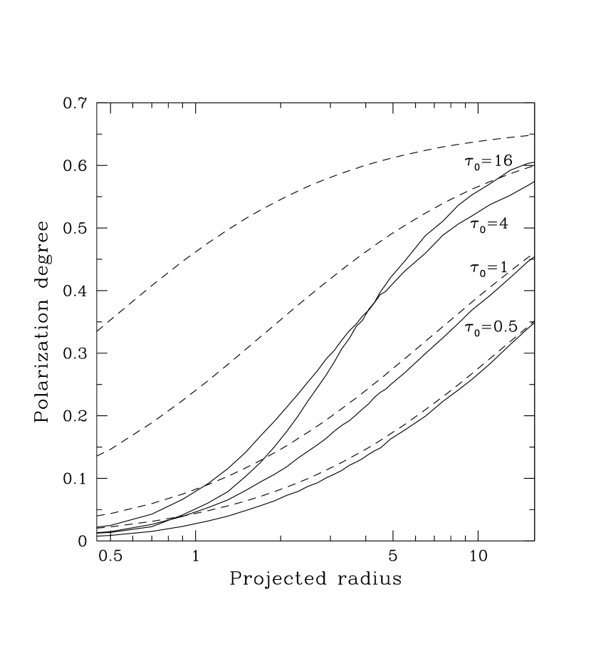
Figure 3: Same as Fig. 1, but for $\beta=1$. The dashed curves are $\rho\rightarrow\infty$ asymptotes calculated from equation (19).

Figure 4: Same as Fig. 2, but for $\beta=1$.

Figures (1)–(4) show a set of Monte-Carlo radial profiles of the Stokes parameter $Q$ and surface brightness $B$ as well as the degree of polarization $P$ for two $\beta$ values: $2/3$ and $1$. We see that $P$ grows monotonically with increasing $\rho$, being negligible near the cluster center and approaching at $\rho\gg 1$ the asymptote given by equation (18) or equation (19) if $\beta=2/3$ or $\beta=1$, respectively. In the former case, this asymptote is a constant, while when $\beta=1$, the polarization grows proportionally to $\rho$ until the projected distance becomes sufficiently large that the radiation scattered into our line of sight begins to dominate the surface brightness (see the denominator of the expression (19)). The polarization at a given $\rho$ also grows with increasing optical depth $\tau_{0}$ until, again, at a certain value of $\tau_{0}\sim 10$ the scattered emission becomes prevailing and $P$ does not increase anymore.

The effect of multiple resonant scatterings is apparent in the central region of the cluster ($\rho\mathrel{\hbox{\hbox to0.0pt{\hbox{\lower 4.0pt\hbox{$\sim$}}\hss}\hbox{$<$}}}$ a few), where the degree of polarization decreases as $\rho\rightarrow 0$ even faster than given by the asymptotic formulae (20) and (21) when $\tau_{0}\mathrel{\hbox{\hbox to0.0pt{\hbox{\lower 4.0pt\hbox{$\sim$}}\hss}\hbox{$>$}}}1$.

Figure 5: Degree of polarization in a resonance line as a function of projected distance from the center of a beta-cluster for different values of the $\beta$-parameter and $\tau_{0}=1$.

Figure 6: Signal-to-noise ratio (defined as $Q/\sqrt{B}$) in detecting polarization in a resonance line from a beta-cluster as a function of projected radius for two valus of the central optical depth and different $\beta$ values: $2/3$ (the solid line), 1 (the dashed line) and 0.5 (the dotted line).

Figure 7: Degree of polarization as a function of photon energy across the spectrum of a resonance line with $\tau_{0}=4$ for a beta-cluster with $\beta=2/3$ at different projected distances from the cluster center. The solid lines result from accurate Monte-Carlo calculations. The dashed lines were obtained assuming complete energy redistribution in scattering. The curves corresponding to the innermost region $\rho<0.5$ were multiplied by 4 to make the trough centered on $E=E_{0}$ visible.

Let us now explore how the polarization effect depends on the $\beta$-parameter when its value is allowed to vary in a broader range. Fig. 5 compares a set of radial profiles of $P$ obtained for different $\beta$ values and a given $\tau_{0}=1$. As expected, the degree of polarization diminishes with decreasing $\beta$ as the cluster emission becomes less centrally peaked and the radiation field permeating the intracluster gas becomes more isotropic. Far from the cluster core, the degree of polarization is a weak declining function of $\rho$ when $1/2<\beta<2/3$. Indeed, in this case $P(\rho\gg 1)\approx Q/B_{0}\sim\tau_{0}\rho^{3\beta-2}$ in accordance with equations (15)–(17). For example, $P(\rho\gg 1,\beta=0.6)\sim\tau_{0}\rho^{-0.2}$.

The degree of polarization remains a declining function of $\rho\gg 1$ also when $\beta<1/2$. In this case the core region no longer dominates the radiation field within the cluster and polarization is mainly caused by the large-scale angular anisotropy of the radiation field. Although this case is not easily analytically treatable, we may expect that $Q\sim B_{\rm in}\sim\tau(\rho)B_{0}$ and $P(\rho\gg 1)\approx Q/B_{0}\sim\tau(\rho)\sim\tau_{0}\rho^{-3\beta+1}$. For example, $P(\rho\gg 1,\beta=0.4)\sim\tau_{0}\rho^{-0.2}$, the same dependence as in the case of $\beta=0.6$. It is clear from the profiles shown in Fig. 5 that when $\beta<2/3$, the polarization degree can be roughly described by a constant value at $\rho\mathrel{\hbox{\hbox to0.0pt{\hbox{\lower 4.0pt\hbox{$\sim$}}\hss}\hbox{$>$}}}5$ which depends on $\beta$ and $\tau_{0}$.

Given the fact that the degree of polarization is an increasing function of $\rho$ at least within a few core radii from the cluster center while the surface brightness falls off with moving away from the cluster core, we may anticipate that there should exist a range of projected radii favorable from the point of view of detectibility of the polarized signal. In order to check this suggestion we have plotted in Fig. 6 the signal-to-noise ratio, which is proportional to $Q/\sqrt{B}$, as a function of $\rho$. In doing so we, of course, assumed that the contribution of the instrumental and cosmic background to the detected X-ray flux is negligible. One can see that the region $0.5\mathrel{\hbox{\hbox to0.0pt{\hbox{\lower 4.0pt\hbox{$\sim$}}\hss}\hbox{$<$}}}\rho\mathrel{\hbox{\hbox to0.0pt{\hbox{\lower 4.0pt\hbox{$\sim$}}\hss}\hbox{$<$}}}10$ centered (on a logarithmic scale) at $\rho_{0}\sim 2$ is most suitable for measurements with future X-ray polarimeters, with the expected degree of polarization being $\sim 10\beta^{2}\tau_{0}$ per cent at $\rho_{0}=2$ for $0.5<\beta<1$ and $\tau_{0}<2$.

Although in obtaining the numerical results described above we treated the process of resonant scattering accurately, assuming complete energy redistribution in scatterimg leads to virtually the same results. This is demonstrated in Fig. 7, where we have plotted the degree of polarization as a function of photon energy for different projected radii. Note that in the considered case of a moderate optical depth ($\tau_{0}=4$), $P$ is somewhat higher in the wings of the resonance line than at its center for the spectrum taken from the cluster core region, while the polarization is approximately constant across the line spectra measured at $\rho\gg 1$.

2.2.2 Beta-cluster with a central cooling flow or AGN

We might expect that the net degree of polarization would be larger for clusters with a luminous cooling flow. Observed X-ray surface brightness profiles of cooling flows usually imply an approximately $1/r$ radial density law for the X-ray emitting gas which probably flattens out at $r\mathrel{\hbox{\hbox to0.0pt{\hbox{\lower 4.0pt\hbox{$\sim$}}\hss}\hbox{$<$}}}$ a few kpc. Therefore, when considering a cooling-flow beta-cluster, one possibility is to represent the cooling flow by an additional beta-model with $\beta\approx 1/3$ and a small core-radius $r_{\rm c}$.

At the same time, it is illuminating to consider this situation as though we have a beta-cluster with total luminosity $L_{\beta}$ in a given line and a point source in the cluster center with a luminosity $L$ in the same line. Clearly, the results of such modelling will be applicable only at projected radii larger than the effective size of the cooling flow (typically at $\rho\mathrel{\hbox{\hbox to0.0pt{\hbox{\lower 4.0pt\hbox{$\sim$}}\hss}\hbox{$>$}}}$ a few tens of kpc).

At the same time the results reported below are applicable to another important situation in which there is a strong active galaxy (AGN) in the center of a beta-cluster. In this case $L$ will represent the luminosity of resonantly absorbed radiation from the AGN continuum (power-law) spectrum in a given X-ray line.

To find the contribution of the central point source to the surface brightness and polarization in the single-scattering approximation we must substitute

$$I({\bf r_{0}},{\bf\Omega})=\frac{L}{4\pi r_{0}^{2}}\delta({\bf\Omega}-{\bf r_{0}}/r_{0}),$$ (22)

into equations (8)–(10), which leads to the results given below.

Isotropic scattering

If $\beta=2/3$,

$$B_{\rm in}=\frac{\sqrt{2}}{16\pi^{2}}\frac{L\tau_{0}}{r_{\rm c}^{2}}\left(\frac{1}{\rho}-\frac{1}{\sqrt{1+\rho^{2}}}\right),\,\,\,Q=0.$$ (23)

If $\beta=1$,

$$B_{\rm in}=\frac{\sqrt{2}}{32\pi^{2}}\frac{L\tau_{0}}{r_{\rm c}^{2}}\left(\frac{\pi}{\rho}-\frac{2}{1+\rho^{2}}-\frac{2\arctan\rho}{\rho}\right),\,\,\,Q=0.$$ (24)

Dipole scattering

If $\beta=2/3$,

$$B_{\rm in}=\frac{3\sqrt{2}}{128\pi^{2}}\frac{L\tau_{0}}{r_{\rm c}^{2}}\left(\frac{3+2\rho^{2}}{\rho}-\frac{4+2\rho^{2}}{\sqrt{1+\rho^{2}}}\right),$$

$$Q=\frac{3\sqrt{2}}{64\pi^{2}}\frac{L\tau_{0}}{r_{\rm c}^{2}}\left(\frac{1-2\rho^{2}}{2\rho}+\frac{\rho^{2}}{\sqrt{1+\rho^{2}}}\right).$$ (25)

If $\beta=1$,

$$B_{\rm in}=\frac{3\sqrt{2}}{128\pi^{2}}\frac{L\tau_{0}}{r_{\rm c}^{2}}\left(-\frac{5+3\rho^{2}}{1+\rho^{2}}+\frac{3(1+\rho^{2})}{\rho}\arctan\frac{1}{\rho}\right),$$

$$Q=\frac{3\sqrt{2}}{128\pi^{2}}\frac{L\tau_{0}}{r_{\rm c}^{2}}\left(\frac{1+3\rho^{2}}{1+\rho^{2}}+\frac{1-3\rho^{2}}{\rho}\arctan\frac{1}{\rho}\right).$$ (26)

One can see that the effect of a particular phase function (isotropic or dipole) on the surface-brightness profile of scattered emission is quite small even in the case under consideration, where we are dealing with a compact (not diffuse as in the case of a self-illuminating beta-cluster) illuminating source. In particular if $\beta=2/3$, $I^{\rm dip}_{\rm scat}/I^{\rm iso}_{\rm scat}=9/8$ for $\rho\rightarrow 0$ and $15/16$ for $\rho\rightarrow\infty$. If $\beta=1$, $I^{\rm dip}_{\rm scat}/I^{\rm iso}_{\rm scat}=9/8$ for $\rho\rightarrow 0$ and $9/10$ for $\rho\rightarrow\infty$.

Figure 8: Polarization degree in a resonance line with $\tau_{0}=1$ as a function of projected radius for a $\beta=0.5$ beta-cluster with a point source in the center for different ratios of the luminosity of the central source ($L$) to the total luminosity of the cluster $L_{\beta}$ in the line.

Figure 9: Same as Fig. 8, but for $\beta=2/3$. Also shown is the analytic result (25) valid in the small optical depth limit ($\tau_{0}\ll 1$).

If we ignore for the moment the resonant scattering of the beta-cluster emission, then the total observed surface brightness will be $B=B_{0}+B_{\rm in}$ and the corresponding polarization degree $P=Q/(B_{0}+B_{\rm in})$, with $B_{0}$ being given by equation (7). In the vicinity of the central source (at $\rho\ll 1$) the surface brightness will be dominated by the scattered emission, so that $P=Q/B_{\rm in}$. In the case of dipole scattering, $P\rightarrow 1/3$ when $\rho\rightarrow 0$ for arbitrary values of $\beta$. The polarization at large projected radii ($\rho\gg 1$), will depend on the ratio $B_{\rm in}/B_{0}\sim(L/L_{\beta})\tau_{0}\rho^{3\beta-2}$. This ratio is growing with distance from the cluster center for $\beta>2/3$, and declining in the opposite case.

If the condition $B_{\rm in}\gg B_{0}$ is indeed met, then

$$P(\rho\gg 1)=\frac{1}{1+\Gamma(3\beta/2+1/2)/\Gamma(3\beta/2+3/2)}.$$ (27)

This relation follows directly from equations (14), (15) and (17), which were originally derived for the ideal beta-cluster assuming that its entire luminosity was emitted from its center. In particular, $P(\rho\gg 1,\beta=2/3)=3/5$, $P(\rho\gg 1,\beta=1)=2/3$.

Figs. 8 and 9 show the results of our numerical simulations for the model of a beta-cluster with a point central source. One can see that deep within the cluster core the degree of polarization approaches the value $1/3$ as $\rho\rightarrow 0$, in agreement with the analytic result, because the radiation field is completely dominated by emission from the point source. When we move away from the core region to $\rho\mathrel{\hbox{\hbox to0.0pt{\hbox{\lower 4.0pt\hbox{$\sim$}}\hss}\hbox{$>$}}}$ a few, provided that $\beta>1/2$, we effectively come to a situation in which there is a point central source with total luminosity $L_{\rm tot}=L+L_{\beta}$ whose emission is scattered by the beta-cluster. The resulting $P(\rho)$ profile is then a function of $L/L_{\beta}$. If $\beta>2/3$, $P$ approaches as $\rho\rightarrow\infty$ the asymptotic value characterizing the point-source case: $3/5$ if $\beta=2/3$ and $2/3$ when $\beta=1$. If $\beta<1/2$, the role of the central point source becomes unimportant at $\rho\gg 1$, similarly to the role of the beta-cluster core, as discussed in §2.2.1.

We see from Figs. 8 and 9 that already at $L=0.5L_{\beta}$ the observed line emission is strongly polarized across the whole cluster, with $P$ being of the order of 15% when $\tau_{0}=1$.

3 Implications for observations

Let us now discuss the prospects of observing the resonant scattering polarization effect in actual clusters of galaxies. We shall begin by discussing potentially interesting X-ray lines and then continue by performing numerical simulations for a few clusters.

3.1 Most promising lines

For the discussion below as well as for the calculations in §3.2 it is important that given the very low density of the intracluster gas, virtually all ions are in their ground atomic state. In particular, only the lowest fine-structure sublevels are populated.

3.1.1 He-like $K_{\alpha}$ line

The resonant transition $1s^{2}-1s2p(^{1}P_{1})$ at 6.7 keV of He-like iron corresponds to one of the most prominent lines in the spectra of rich clusters of galaxies. He-like iron is abundant in a wide range of temperatures from 1.5 to 10 keV. Taking into account that the transition has a large absorption oscillator strength of $\sim 0.7$, the expected optical depth in the line can be large, and therefore this line is one of the prime candidates for observing the resonant scattering effect. Since the transition corresponds to the change of the total angular momentum from 0 to 1, the phase function of the scattering is a pure dipole. This means that this line is also expected to have highest degree of polarization.

In the vicinity of this line there are several other lines including the intercombination $1s^{2}-1s2p(^{3}P)$ and forbidden $1s^{2}-1s2p(^{3}S)$ lines of He-like iron and many dielectronic satellite lines. For the forbidden line the optical depth is essentially zero, while for the most important intercombination line ($1s^{2}-1s2p(^{3}P_{1})$) the absorption oscillator strength is at least a factor of 10 lower than for the resonant line. While many of the satellite lines have a vanishing optical depth, some satellite lines do have an appreciable oscillator strength. The latter correspond to the singly exited state of particular ions of iron (e.g. the transitions $1s^{2}2s-1s2s2p$ for Li-like iron). However, Li-like iron is present in sufficient amounts only in a relatively cool (below 4 keV) plasma, which implies that in hot clusters the optical depth in these lines will be lower than for the resonant He line. Note also that for the satellite lines autoionization of electrons (from the exited state) plays a role, thus suppressing the emission in the satellite line in the case of a sufficient optical depth. A similar effect called “resonant Auger destruction” has been considered in application to ionized accretion disks (e.g. Ross, Fabian & Brandt 1996). For clusters this effect is less important because of the relatively low optical depth and lower ratio of autoionization and radiative decay rates (at least for relevant transitions in the Li-like iron).

All these lines (except for dielectronic satellites with a large principal number of the spectator electron in Li-like iron) are separated from the main resonant line by at least 30 eV. Therefore, even turbulent broadening does not severely mix the resonant line with other lines. Finite energy resolution of the polarimeter may, however, significantly affect the prospects of detection of the polarized emission. Assuming that only the resonant line of He-like iron is polarized, the measurable polarization can be estimated by multiplying the degree of polarization as would result in the ideal case (as calculated in §2) by the factor $f=F_{\rm line}/F_{\rm tot}$ where $F_{\rm line}$ is the flux in the resonant line and $F_{\rm tot}$ is the total flux measured by the detector in an energy band $\Delta E$ centered on the resonant line energy. In Fig. 10 we plot this factor as a function of $\Delta E$ for two values of the plasma temperature of 8 and 2 keV. One can see that the energy resolution of a CCD-type detector is needed to avoid a strong decrease in polarization due to contamination by the unpolarized flux in the continuum and other lines.

Figure 10: Decrease of the observed degree of polarization for an instrument collecting photons in a given energy range centered on the He-like line at 6.7 keV. The solid and dotted lines correspond to a plasma temperature of 8 and 2 keV, respectively. The abundance of iron was assumed to be 0.5 solar. Only the flux in the line is assumed to be polarized. The edges in the curves correspond to such widths of the energy window when an additional prominent line falls inside the window.

3.1.2 He-like $K_{\beta}$ iron line

This line ($1s^{2}-1s3p(^{1}P_{1})$) at 7.88 keV is very similar to the $K_{\alpha}$ line, but the oscillator strength is $\sim 0.16$, i.e. a factor of 4.5 smaller. This directly translates into the optical depth being smaller by the same factor. It was suggested (e.g. Akimoto et al. 1997; Molendi 1998) that the comparison of the radial profiles in the $K_{\alpha}$ and $K_{\beta}$ lines may be used as an indicator of the resonant scattering in clusters. Note, however, that the different energies of these two lines imply some dependence of the ratio of their emissivities on temperature. This effect may complicate an analysis of real data.

3.1.3 H-like $K_{\alpha}$ iron line

This line at 6.96 keV has two components, $1s-2p(^{1}P_{1/2})$ and $1s-2p(^{1}P_{3/2})$, separated by $\sim 20$ eV. The oscillator strengths of the lines are 0.14 and 0.28 respectively. For the first line the total angular momentum is equal to $1/2$ both for the ground and excited states, and therefore the scattering phase function is isotropic and scattered emission is unpolarized. For the second line the total angular momentum of the exited state is $3/2$ and the phase function is a sum of isotropic and dipole phase functions with equal weights. For the conditions in clusters (i.e. only marginally optically thick cases) all complications associated with the quantum interference of these two lines (e.g. Stenflo 1980) can be safely neglected. We note here that the ratio of the intensities of these two lines is essentially independent of temperature. Therefore, a comparison of the radial profiles and polarization properties of these lines would be the cleanest test for the presence of resonant scattering, should next generation calorimeters and polarimeters allow one to resolve them. However hydrogen-like iron is abundant only in high temperature clusters, and the optical depth is systematically lower than for the He-like resonant line.

3.1.4 $K$-shell lines of lighter elements

For low temperature clusters and especially for cooling flow regions with the gas temperatures in the range of 1–3 keV, the K-shell lines of lighter elements (e.g. Mg, Si or S) may be important. These elements have abundances comparable to the iron abundance and the main limiting factor is the ionization fraction. Compared to iron K-lines, the cross sections (per ion) for these lines are higher – see equations (5), (2) – because of the lower energy of the transition, although the smaller atomic masses imply that Doppler broadening is more important for these elements than for iron (and as a consequence turbulent broadening has less impact on these lines than on iron K-lines).

3.1.5 $L$-shell lines of iron

The $L$-shell transitions (e.g. of the $2s-3p$ or $2p-3d$ type) with energies of the order of 1 keV are especially strong at lower temperatures of 1–3 keV typical for cooling flow regions. They are associated with Li-, Be-, B-, C-, N-, O-, F- and Ne-like ions of iron. At any given temperature several ionization stages are present and several strong lines are present. Polarization properties of these transitions depend on the total angular momenta of the ground and excited states.

Several lines appear particularly promising and interesting for polarimetric studies. At temperatures of the order of 1 keV this is the Be-like iron line at 1.129 keV which has a large oscillator strength ($f=0.7$) and a pure dipole scattering phase function. At still lower temperatures $\sim 0.5$ keV the most interesting is the Ne-like iron (Fe XVII) line at 0.825 keV which has an exceptionally large oscillator strength ($f=2.95$) and a pure dipole scattering phase function. We note however that it is not clear if the gas in this temperature range is abundant in cluster cooling flows. The standard models do predict such low-temperature plasma, while recent Chandra and XMM observations [Böhringer et al. 2002] do not provide clear evidence for it.

3.2 Individual clusters

We have performed Monte-Carlo calculations to simulate the resonant scattering polarization effect in three prototypical clusters of galaxies. The line energies and oscillator strengths were taken from the list of strong resonant lines of Verner, Verner & Ferland [Verner, Verner & Ferland 1996]. The solar abundances of elements were taken from Anders & Grevesse [Anders & Grevesse 1989]. We used the MEKAL code [Mewe et al. 1986, Mewe et al. 1986, Kaastra 1992, Liedahl et al. 1995] as implemented in the software package XSPEC v10 [Arnaud 1996] to calculate plasma emissivity in a given line as a function of radius. The ionization fractions were calculated using collisional ionization rate fits from Voronov [Voronov 1997], radiative recombination rates from Verner & Ferland [Verner & Ferland 1996] and dielectronic recombination rates from Aldrovandi & Pequignot [Aldrovandi & Pequignot 1973], Shull & van Steenberg [Shull & van Steenberg 1982] and Arnaud & Rothenflug [Arnaud & Rothenflug 1985]. We note here that this usage of several independent sources of atomic data may lead to certain inconsistencies in the resulting values of the polarization degree, but we believe that the net effect (of these inconsistencies) is very minor and can be neglected.

3.2.1 Coma cluster

The Coma cluster is the prototype of a rich regular cluster. The temperature of the gas is $kT=8.1$ keV and its density distribution is described by the beta-law (1) with $\beta=0.67$, $r_{\rm c}=430$ kpc and $N_{0}=2.3\times 10^{-3}$ cm^-3 [Jones & Forman 1999]. According to recent XMM-Newton observations the abundance of iron is 0.25 relative to the solar value [Arnaud et al. 2001]. At the given gas temperature He-like and H-like ions of iron are present in nearly equal amounts with a negligible admixture of less ionized atoms. Given the oscillator strengths of the corresponding lines, only the 6.7 keV line of He-like iron proves to have a substantial optical depth to resonant scattering, as indicated in Table 1.

The reported values of $\tau_{0}$ were calculated assuming ${\mathcal{M}}=0$. The optical depth will be smaller is we adopt a more realistic ${\mathcal{M}}>0$ value, because turbulent broadening is especially important for iron, as follows from equation (2). For example, $\tau_{0}=0.18$ for the 6.7 keV line when ${\mathcal{M}}=0.2$. Fig. 11 shows the expected radial profile of the degree of polarization in the 6.7 keV line as would be measured by a polarimeter with perfect spectral resolution. We see that $P\mathrel{\hbox{\hbox to0.0pt{\hbox{\lower 4.0pt\hbox{$\sim$}}\hss}\hbox{$<$}}}5$% is expected. The polarization would be a little smaller when measured by a detector having a finite spectral resolution, as is clear from Fig. 10.

Table 1: X-ray lines with significant optical depth ($\tau_{0}>0.05$) to resonant scattering. The Coma cluster.

Ion	Energy	Optical depth	Weight of dipole
	(keV)		scattering
Fe XXIV	1.163	0.04	0
Fe XXIV	1.168	0.07	0.5
Fe XXV	6.700	0.37	1
Fe XXV	7.881	0.06	1
Fe XXVI	6.952	0.05	0
Fe XXVI	6.973	0.09	0.5

Figure 11: Polarization degree in the most prominent resonant line as a function of projected distance from the center of the Coma cluster. The solid line corresponds to the case of negligible turbulence in the gas, while the ratio of the characteristic turbulent velocity to the sound velocity is ${\mathcal{M}}=0.2$ and ${\mathcal{M}}=0.4$ for the dotted and dashed line, respectively.

3.2.2 Perseus cluster (A426)

The X-ray emission of the Perseus cluster is peaked on the central dominant galaxy NGC 1275, suggesting the presence of a cooling flow.

We adopted simple analytic expressions for the radial dependence of density and temperature in this cluster. The overall density distribution, including the central cooling flow region, was described by a single beta-model (1) with the parameters $N_{0}=0.03$ cm^-3, $\beta=0.47$ and $r_{\rm c}=47$ kpc. The temperature distribution was set to

$$kT=7\frac{1+(r/r_{0})^{3}}{2.3+(r/r_{0})^{3}}\,\,\,{\rm keV},$$ (28)

with $r_{0}=100$ kpc. The gas is coldest at the cluster center, where $kT=3$ keV, and hottest in the outermost regions, reaching $kT=7$ keV. The above distributions approximately correspond to the deprojected density and temperature profiles derived from XMM-Newton data (to be published elsewhere). Given the substantial azimuthal asymmetry of the Perseus cluster, these azimuthly averaged distributions can be used only for crude estimates. Note that outside the cooling flow (at $r>300$ kpc) the density radial profile we use approximately matches the beta-profile inferred from Einstein observations [Jones & Forman 1999], defined by values $N_{0}=4.1\times 10^{-3}$ cm^-3, $\beta=0.58$ and $r_{\rm c}=280$ kpc. The ratio of the two profiles is less than 1.5 up to a distance of 4 Mpc.

We have adopted a constant abundance of iron across the cluster of 0.5 solar, as inferred from the XMM-Newton spectroscopic data.

Table 2: X-ray lines with large optical depth ($\tau_{0}>0.5$) to resonant scattering. The Perseus cluster.

Ion	Energy	Optical depth	Weight of dipole
	(keV)		scattering
Fe XXIV	1.163	0.8	0
Fe XXIV	1.168	1.6	0.5
Fe XXV	6.700	3.3	1
Fe XXV	7.881	0.5	1

Table 2 lists resonant lines for which $\tau_{0}>0.5$ (at ${\mathcal{M}}=0$). We see that the 6.7 keV line is again the one with the largest optical depth. In contrast to the previous example, Li-like iron is fairly abundant in the Perseus cluster, particularly in its cooling flow, which gives rise to a moderate optical depth in the Fe XXIV doublet at 1.17 keV. Fig. 12 shows the simulated radial profiles for the degree of polarization in the lines listed in Table 2. In the case of the 1.17 keV doublet, the polarization degree was found as $P=(Q_{1}+Q_{2})/(B_{1}+B_{2})$ (with $Q_{1,2}$ and $B_{1,2}$ being the corresponding quantities for each of the two lines). This calculation assumes that the polarimeter used cannot resolve the lines. Note that Doppler broadening is not sufficient to cause these lines to overlap even at sonic turbulence (${\mathcal{M}}=1$):

$$\Delta E_{\rm D}=0.5\left[\frac{kT}{5\,{\rm keV}}(1+78M^{2})\right]^{1/2}\,\,\,{\rm eV},$$ (29)

compared with the $4.6$ eV splitting of the doublet.

We see from Fig. 12 that the expected degree of polarization is high for the 6.7 keV line – larger than 8% at $\rho>300$ kpc. The polarization is a factor of 5 smaller for the 7.88 keV and 1.17 keV lines. This is caused by the smaller optical depth and in the latter case also by the lower weight of dipole scattering. We also see that the degree of polarization is nearly constant outside the central $300$ kpc for all three sampled lines, which is in agreement with the results of §2.

Figure 12: Same as Fig. 11, but for the Perseus cluster.

3.2.3 M87/Virgo cluster

This is another example of a cooling flow cluster, but in this case the characteristic temperature of the cooling flow is lower ($kT\sim 1.5$ keV in the center) than in the preceeding example. For our computations we have adopted gas distribution parameters as inferred from XMM-Newton and ROSAT observations [Nulsen & Boehringer 1995, Böhringer et al. 2001, Mathews et al. 2001]. Namely, the density distribution within the central 12 kpc is represented by a beta-model with $\beta=0.47$, $N_{0}=0.35$ cm^-3 and $r_{\rm c}=2.0$ kpc. At larger distances, a less steep density law is used:

$$N_{\rm e}=0.12\left[1+\left(\frac{r}{4.3\,\mathrm{kpc}}\right)^{1.18}\right]^{-1},$$ (30)

which is approximately a beta-law with $\beta_{2}=0.39$.

The overall gas temperature distribution is approximated by

$$T=T_{0}\left[\frac{1}{1+(r/\,13.2\,\mathrm{kpc})}+0.20\left(\frac{r}{13.2\,\mathrm{kpc}}\right)^{0.22}\right]^{-1}.$$ (31)

The temperature rises from the center, where $T_{0}=1.3$ keV, towards a broad maximum of $T=3.0$ keV at $r\sim 150$ kpc.

The element abundances are assumed to be constant at $r<10$ kpc, being $F(\mathrm{O})=0.4$, $F(\mathrm{Si})=1.0$, $F(\mathrm{S})=1.0$, $F(\mathrm{Ar})=1.0$, $F(\mathrm{Ca})=1.0$ and $F(\mathrm{Fe})=0.7$ (in units of solar abundances), then gradually falling with radius to reach the values $F(\mathrm{O})=0.4$ (unchanged), $F(\mathrm{Si})=0.6$, $F(\mathrm{S})=0.6$, $F(\mathrm{Ar})=0.6$, $F(\mathrm{Ca})=0.6$ and $F(\mathrm{Fe})=0.35$ at $r=40$ kpc, and remain constant from there on.

Table 3: X-ray lines with large optical depth ($\tau_{0}>0.5$) to resonant scattering. The M87/Virgo cooling flow.

Ion	Energy	Optical depth	Weight of dipole
	(keV)		scattering
O VIII	0.654	0.4	0
O VIII	0.654	0.7	0.5
Ne X	1.021	0.5	0
Ne X	1.022	1.0	0.5
Si XIII	1.865	2.1	1
Si XIV	2.004	0.8	0
Si XIV	2.006	1.7	0.5
S XV	2.461	2.5	1
S XVI	2.620	0.3	0
S XVI	2.623	0.6	0.5
Ar XVII	3.140	0.8	1
Fe XX	0.967	0.7	0.28
Fe XX	0.967	0.5	0.32
Fe XXI	1.009	2.3	1
Fe XXII	1.053	3.3	0.5
Fe XXII	1.064	0.5	0
Fe XXII	1.084	1.5	0.5
Fe XXIII	1.129	6.2	1
Fe XXIII	1.493	1.2	1
Fe XXIV	1.163	1.6	0
Fe XXIV	1.168	3.2	0.5
Fe XXIV	1.553	0.6	0.5
Fe XXV	6.700	1.8	1

Table 3 gives a list of potentially interesting lines for observing the resonant scattering polarization effect. There are in total 17 lines (if counting fine-structure multiplets as a single line) with optical depth to resonant scattering exceeding 0.5. Most of these lines, including the lines of elements lighter than Si, the lines of He-like Si and S, and those of Fe ionic species less ionized than Fe XXIV originate preferentially within a few tens of kpc from the M87 center where the temperature is sufficiently low. The most interesting line is the one at 1.129 keV, which corresponds to the $2s-3p$ transition in Be-like iron. This line has the largest optical depth and a dipole scattering phase function. Also notable are the $K\alpha$ lines of helium-like Si and S at $1.865$ and $2.461$ keV, respectively. These lines are well separated on the spectrum from the Fe $L$-shell complex of lines and the detection of polarization in them does not require a high spectral resolution of the polarimeter.

Fig. 13 shows the simulated radial profiles of the degree of polarization for several prominent lines. As expected, the highest polarization is achieved in the Fe XXIII 1.129 keV line, reaching a maximum of 14% (at ${\mathcal{M}}=0$) very close to the cooling flow center (at $\rho\sim 15$ kpc), where the surface brightness is still large. The polarization degree falls off from this maximum with moving away from the center, and a similar behaviour pertains to the other lines, excluding the lines of Li-like (e.g. the one at 1.17 keV) and He-like iron (6.7 keV), which are characterized by increasing $P$ with projected radius. The case of the 1.129 keV line and other similar lines closely corresponds to our model of a point source in the center of a beta-cluster considered in §2.2.2. Indeed, the fraction of the overall line luminosity emitted within the central 10 kpc is as large as 33% for the Fe XXIII 1.129 keV line, 33% for the Si XIII 1.865 keV line, 19% for the S XV 2.460 keV line, 73% (!) for the Fe XXI 1.009 keV line; is only 15% for the Fe XXIV 1.17 keV and as small as 2% for the Fe XXV 6.7 keV line.

Given the large number of resonant lines with a significant optical depth from different elements and ionization species together with the proximity to us, the M87/Virgo cluster appears to be a perfect target for future X-ray polarimetric observations. It is clear that the projected radial profiles shown in Fig. 13 should be very sensitive to the temperature, density and abundance physical radial profiles.

Figure 13: Same as Fig. 11, but for the M87 cooling flow.

4 Conclusions

• We have shown that the expected degree of polarization for the brightest X-ray lines from clusters of galaxies is of the order of 10%.

• The degree of polarization is a function of projected distance from the cluster center, and the polarization vector is perpendicular to the projected radius vector. This implies in particular that the integrated X-ray flux from the whole cluster will be unpolarized (provided the cluster if spherically symmetric).

• It has also been demonstrated that for regular clusters, whose gas density distribution obeys the beta-law (1), the largest signal-to-noise ratio in measuring the polarization signal is attainable in the range of projected radii between $0.5$ and $10$ core-radii. The degree of polarization is zero in the direction of the cluster center, while the photon flux from the outer parts is small making it difficult to measure the polarization.

• Rich regular clusters as well as clusters with a dominant cooling flow are the best targets for future polarimetric observations.

Why is it important to observe the polarization effect? First of all, this effect is unique in the sense that there is no other obvious mechanism that could lead to polarization in X-ray lines. Thus, a detection of polarized diffuse emission in an X-ray line would be a solid proof that resonant scattering is indeed in operation.

As mentioned before, resonant scattering affects the “apparent” (inferred under the assumption of optically thin emission) element abundance radial profiles of clusters [Gilfanov et al. 1987a, Shigeyama 1998]. As a consequence, in order to determine the true abundance profiles from spectroscopic measurements, one should be able to accurately subtract the distortions caused by resonant scattering, which can well be larger in magnitude than the true underlying radial trend. This is a difficult task, because the surface brightness is an integral characteristic of a given line of sight which passes through regions with different densities and temperatures. One way to proceed is to compare the surface brightness profiles of at least two spectral lines corresponding to a given element (e.g. $K\alpha$ and $K\beta$ lines of iron, see Akimoto et al. 1997; Molendi 1998). Polarimetric measurements could significantly simplify such an analysis, for measuring of the polarized flux in a single line already allows one to estimate the contribution of resonant scattering to apparent abundance profiles. Apart from element abundances, the resonant scattering effects in principle can provide information on the velocity field within the cluster, because the optical depth in a given line is a function of the characteristic velocity of the corresponding ions. Lines of iron are particularly sensitive to the velocity of turbulent motions.

Finally, the polarization effect can also be used for cosmological purposes. Indeed, since the surface brightness of resonantly scattered emission and of its polarized component is roughly proportional to the optical depth along a given line of sight while the surface brightness of continuum thermal emission is proportional to the integral of the density squared along the line of sight, it is possible to determine the distance to the cluster and consequently the Hubble constant analogously as is done using resonance X-ray absorption lines [Krolik & Raymond 1988, Sarazin 1989] or the cosmic microwave background (the Sunayev-Zel’dovich effect).

There are obvious requirements to a future X-ray polarimeter. First, it should have the sufficient angular resolution to probe individual parts of a cluster (we recall that the polarization vanishes when integrated over the whole cluster). Second, the CCD-type energy resolution is desirable in order to avoid significant contamination of the polarized emission of a resonance line by the unpolarized emission of neighbouring lines and the continuum. Finally, a large effective area of the telescope is needed, larger than is required for the detection of unpolarized resonantly scattered emission, since the expected degree of polarization is $\sim 10$%.

5 Acknowledgements

This research was partially supported by the Russian Foundation for Basic Research (projects 00-02-16681 and 00-15-96649) and by the program of the Russian Academy of Sciences ”Astronomy (Nonstationary astronomical objects)”. RS as a Gordon Moore Scholar thanks Caltech for hospitality during the completion of this paper.

References

- [Akimoto et al. 1997] Akimoto F. et al., 1997, in X-ray Imaging and Spectroscopy of Cosmic Plasmas, ed. F. Makino & K. Mitsuda (Tokio: Universal Academy Press), 95
- [Aldrovandi & Pequignot 1973] Aldrovandi S.M.V. & Pequignot, D., 1973, A&A, 25, 137
- [Anders & Grevesse 1989] Anders E. & Grevesse N., 1989, Geochimica et Cosmochimica Acta, 53, 197
- [Arnaud & Rothenflug 1985] Arnaud M. & Rothenflug M., 1985, A&AS, 60, 425
- [Arnaud & Raymond arnray1992] Arnaud M. & Raymond J., 1992, ApJ, 398, 394
- [Arnaud 1996] Arnaud K.A., 1996, Astronomical Data Analysis Software and Systems V, eds. Jacoby G. and Barnes J., ASP Conf. Series volume 101, 17
- [Arnaud et al. 2001] Arnaud M. et al., 2001, A&A, 365, L67
- [Basko et al. 1981] Basko M.M., Komberg B.V., Moskalenko E.I., 1981, Sov. Astron., 25, 402
- [Böhringer et al. 2001] Böhringer H., Belsole E., Kennea J. et al., 2001, A&A, 365, 181
- [Böhringer et al. 2002] Böhringer H., Matsushita K., Churazov E., Ikebe Y., Chen Y., 2002, submitted to A&A (astro-ph/0111112)
- [Cavaliere & Fusco-Femiano 1976] Cavaliere A. & Fusco-Femiano R., 1976, A&A, 49, 137
- [Chandrasekhar 1950] Chandrasekhar, S., 1950, Radiative Transfer, Oxford, Clarendon Press, 1950
- [Costa et al. 2001] Costa E., Soffitta P., Bellazzini R., Brez A., Lumb N. & Spandre G., 2001, Nature, 411, 662
- [David 2000] David L.P., 2000, ApJ, 529, 682
- [Gilfanov et al. 1987a] Gilfanov M.R., Sunyaev R.A. & Churazov E.M., 1987a, Sov. Astron. Lett., 13, 3
- [Gilfanov et al. 1987b] Gilfanov M.R., Sunyaev R.A. & Churazov E.M., 1987b, Sov. Astron. Lett., 13, 233
- [Hamilton 1947] Hamilton D.R., 1947, ApJ, 106, 457
- [Jones & Forman 1999] Jones C. & Forman W., 1999, ApJ, 511, 65
- [Kaastra 1992] Kaastra J.S., 1992, An X-Ray Spectral Code for Optically Thin Plasmas (Internal SRON-Leiden Report, updated version 2.0)
- [Krolik & Raymond 1988] Krolik J.H., Raymond J.C., 1988, ApJ, 335, L39
- [Liedahl et al. 1995] Liedahl D.A., Osterheld A.L. and Goldstein W.H., 1995, ApJL, 438, 115
- [Mathews et al. 2001] Mathews W.G., Buote D.A., & Brighenti F., 2001, ApJL in press (astro-ph/0101545)
- [Mewe et al. 1986] Mewe R., Gronenschild E.H.B.M. and van den Oord G.H.J., 1985, A&AS, 62, 197
- [Mewe et al. 1986] Mewe R., Lemen J.R. and van den Oord G.H.J., 1986, A&AS, 65, 511
- [Molendi et al. 1998] Molendi S. et al., 1998, ApJ, 499, 608
- [Nulsen & Boehringer 1995] Nulsen P.E.J. & Boehringer H., 1995, MNRAS, 274, 1093
- [Ross et al. 1996] Ross R.R., Fabian A.C. & Brandt W.N., 1996, MNRAS, 278, 1082
- [Sarazin 1989] Sarazin C.L., 1989, ApJ, 245, 12
- [Shapiro & Bahcall 1980] Shapiro P.R., Bahcall J.N., 1980, ApJ, 281, 1
- [Shigeyama 1998] Shigeyama T., 1998, ApJ, 497, 587
- [Shull & van Steenberg 1982] Shull J.M. & van Steenberg M., 1982, ApJS, 48, 95
- [Stenflo 1980] Stenflo J.O., 1980, A&A, 84, 68
- [Sunyaev 1982] Sunyaev R.A., 1982, Soviet Astron. Lett., 8, 175
- [Tawara et al. 1997] Tawara Y. et al., 1997, in X-ray Imaging and Spectroscopy of Cosmic Plasmas, ed. F. Makino & K. Mitsuda (Tokio: Universal Academy Press), 87
- [Verner & Ferland 1996] Verner D.A. & Ferland G.J., 1996, ApJS, 103, 467
- [Verner, Verner & Ferland 1996] Verner D.A., Verner E.M. & Ferland G.J., 1996, Atomic Data and Nuclear Data Tables, 64, 1
- [Voronov 1997] Voronov G.S., 1997, Atomic Data and Nuclear Data Tables, 65, 1