Bias and Conditional Mass Function of Dark Halos Based on the Nonspherical Collapse Model

Abstract

Nonspherical collapse is modelled, under the Zeldovich approximation, by six-dimensional random walks of the initial deformation tensor field. The collapse boundary adopted here is a slightly-modified version of that proposed by Chiueh and Lee (2001). Not only the mass function agrees with the fitting formula of Sheth and Tormen (1999), but the bias function and conditional mass function constructed by this model are also found to agree reasonably well with the simulation results of Jing (1998) and Somerville et al. (2000), respectively. In particular, by introducing a small mass gap, we find a fitting formula for the conditional mass function, which works well even at small time intervals between parent and progenitor halos during the merging history.

1 Introduction

In a hierarchical model, the gravitationally bound objects of the universe formed from mergers of smaller objects into larger ones. An issue of fundamental importance is to understand how gravitational structures, such as galaxies and clusters, are distributed as a function of mass and evolving time. Press & Schechter (1974) provided a simple analytical model (hereafter PS model) to describe the mass distribution of dark halos (mass function). This theory is based on the assumption that the process of gravitational collapse can be approximated by spherical symmetry and it occurs when the mean density contrast of precollapse regions predicted by the linear theory reaches a threshold value $\delta_{c}$. Bond et al. (1991) introduced the excursion set formalism and extended the PS theory to calculations of the conditional mass function, which is closely related to the issue of the linear bias and halo merging histories. Mo & White (1996) used the extended Press-Schechter theory (hereafter EPS) to address the large-scale bias, which concerns how the collapsed halos trace the underlying dark matter. Moreover, the EPS theory is also useful for construction of the merger history of dark halos (Bower 1991; Lacey & Cole 1993, 1994 hereafter LC93, LC94), which concerns the probability that a halo of mass $M_{2}$ at time $t_{2}$ has a progenitor halo of mass $M_{1}$ at earlier time $t_{1}$.

The PS or EPS theory has been tested against N-body simulations (Efstathiou et al. 1988; LC94), and the comparisons suggest that the PS model overestimates the number of halos in low-mass regimes and underestimates it in high-mass regimes. This discrepancy indicates that the spherical collapse model used by the PS theory may be too simplistic. Many researchers have taken the nonspherical collapse process into account to correct this problem (e.g., Bond & Myers 1996; Monaco 1995; Lee & Shandarin 1998; Chiueh & Lee 2001; Sheth, Mo and Tormen 2001). Most of these works are still based on the main idea of the PS theory, and further incorporate either the dynamics of ellipsoids or the Zeldovich approximation (Zeldovich 1970).

The main aims of this paper are to investigate the large-scale bias and conditional mass function by using the nonspherical collapse boundary (hereafter NCB) proposed by Chiueh and Lee (2001). We also test whether the results derived from nonspherical collapse boundary can provide better statistical predictions of dark halos than the EPS model does.

The outline of the paper is as follows. In $\S$ 2, we summerize the PS and EPS theory, and briefly review the Zeldovich approximation and the nonspherical collapse boundary proposed by Chiueh & Lee (2001). In $\S$ 3, we show the algorithm and the results of mass function and large-scale bias of our model. In $\S$ 4, the conditional mass function is derived and the comparison with N-body simulation is presented. In $\S$ 5, the conclusion is given.

2 (Extended) Press-Schechter Formalism

2.1 Mass function

The Press-Schechter theory (1974) assumes that the initial density fluctuations are Gaussian random fields. Let $\delta_{R}(\vec{x})$ denote the overdensity field at position $\vec{x}$ in the comoving coordinate when the density distribution is smoothed over scale R by a window function $W_{R}$. The relation is

$$\delta_{R}(\vec{x})=\int\delta(\vec{x}^{\prime})W_{R}(\vec{x}-\vec{x}^{\prime})d^{3}\vec{x}^{\prime},$$ (1)

with a squared variance

$$S=\sigma^{2}(M)=<|\delta_{R}(\vec{x})|^{2}>=\frac{1}{(2\pi)^{3}}\int p(k)\widetilde{W}_{R}^{2}(k)4\pi k^{2}dk,$$ (2)

where $p(k)$ is the power spectrum of density fluctuations and $\widetilde{W}_{R}(k)$ is the Fourier transform of the window function $W_{R}(\vec{x}-\vec{x}^{\prime})$. The squared variance $S$ increases as mass $M$ decreases, and in this paper, we will often use $S$ to represent the mass scale.

Bond et al. (1991) extended the original PS method and used random walks (or called excursion set) to address the mass function problem. When variance $S$ equals zero, the density contrast $\delta$ is set to zero. As $S$ increases, $\delta$ changes randomly. When $\delta$ first hits the threshold value $\delta_{c}$, the random walk stops and the region of mass scale $S$, over which $\delta$ is smoothed, collapses into a bound object. This prescription is equivalent to a diffusion process with an absorbing boundary at $\delta=\delta_{c}$, which has been solved by Chandrasekhar (1943) when the window function is chosen to be a sharp k-space filter. Thus, one can calculate the probability of a trajectory having its first hit at the threshold $\delta_{c}$ in the mass range between $S$ and $S+dS$ to represent the mass function, which is described by

$$f(S,\delta_{c})dS=\frac{\delta_{c}}{\sqrt{2\pi}S^{3/2}}\mathrm{exp}(-\frac{\delta_{c}^{2}}{2S})dS,$$ (3)

where the functional form $f(x)$ represents the differential probability in the range between $x$ and $x+dx$. Moreover, the (comoving) number density of halos with mass M is

$$\frac{dn}{dM}dM=\frac{\rho_{b}}{M}f(S,\delta_{c})|\frac{dS}{dM}|dM,$$ (4)

where $\rho_{b}$ is the mean mass density of the universe. Alternative choices of window functions, such as real-space top-hat filter and Gaussian filter, are also often used to determine the relation of the squared variance $S$ and mass M. The localized filters yield correlated steps in the above random-walk framework. Comparisons among different types of window function are well discussed by Bond et al. (1991), LC93 and LC94.

For simplicity, we define a variable $\nu\equiv\delta_{c}/S^{1/2}$ and one can easily show that the mass function can be represented as

$$\nu f(\nu)d\nu=\sqrt{\frac{2}{\pi}}\nu\mathrm{exp}(-\frac{\nu^{2}}{2})d\nu.$$ (5)

Here $\delta_{c}$ is often chosen as 1.69, which is predicted by the spherical collapse model. The main advantage of the excusion set approach is that while the mass function depends on the variance $S$ and the value of collapse threshold $\delta_{c}$, the cosmological models enter this problem only through the relation between $S$ and the mass $M$.

Upon comparing with N-body simulations, one finds that the EPS formalism overestimates low-mass and underestimates high-mass halos. Of course one may vary the value of the collapse threshold $\delta_{c}$, but it is not possible to match simulation results well for all mass ranges.

2.2 Conditional mass function

In the picture of the excursion set theory, the conditional probability represents the fraction of trajectories first hitting a higher threshold $\delta_{c1}$ among those trajectories that start from a lower threshold $\delta_{c2}$. In the framework of EPS theory, Lacey & Cole (1993) proposed that the conditional probability can assume a modified form where the origin of the mass function $(0,0)$ shifts to ($S_{2},\delta_{c2}$). Therefore, the conditional probability is simply

$$f(S_{1},\delta_{c1}|S_{2},\delta_{c2})dS_{1}=\frac{(\delta_{c1}-\delta_{c2})}{\sqrt{2\pi}(S_{1}-S_{2})^{3/2}}\mathrm{exp}[-\frac{(\delta_{c1}-\delta_{c2})^{2}}{2(S_{1}-S_{2})}]dS_{1}.$$ (6)

Here, it demands $S_{1}>S_{2}$ and $\delta_{c1}>\delta_{c2}$.

Conditional probability is useful for investigation of large-scale bias as well as merger events of halos. In the first case, the physical meaning of $\delta_{c2}$ is not the collapse threshold at some specific time, but denotes the mean density contrast of a large uncollapsed region of mass scale $S_{2}$. Thus we shall change $\delta_{c2}$ into $\delta_{2}$ to avoid confusion. If we define the bias parameter $b$ to be the fraction of excess dark halos with mass scale $S_{1}$ that can be found in a larger mass scale $S_{2}$, then under the limit $S_{2}\gg S_{1}$ and $\delta_{2}\ll\delta_{c1}$, Mo & White (1996, hereafter MW96) use the EPS formalism to derive that

$$b=\frac{(\delta_{c1}/S_{1}^{1/2})^{2}-1}{\delta_{c1}}=\frac{\nu_{1}^{2}-1}{\delta_{c1}},$$ (7)

where $\nu_{1}\equiv\delta_{c1}/S_{1}^{1/2}$. For convenience, we define a characteristic mass $M^{*}$, which satisfies the requirement $S(M^{*})=\delta_{c1}^{2}$. When $S_{1}<\delta_{c1}^{2}$, i.e., $M_{1}>M^{*}$, the bias factor $b$ is positive, which means the density of halos with masses greater than $M^{*}$ is larger in the denser region of dark matter. On the other hand, when $S_{1}>\delta_{c1}^{2}$, or $M_{1}<M^{*}$, the opposite holds.

In the case of merger events, $\delta_{c2}$ denotes the collapse threshold at a later time $t_{2}$ (as compared with $t_{1}$). Again, the meanings of notations change: $\delta_{c1}\rightarrow\delta_{c}(z_{1}$) and $\delta_{c2}\rightarrow\delta_{c}(z_{2})$, the collapse thresholds at redshifts $z_{1}$ and $z_{2}$, respectively. Thus, $f(M_{1},\delta_{c1}|M_{2},\delta_{c2})dM_{1}$ represents the mass fraction of $M_{2}$ at redshift $z_{2}$ that is in the form of collapsed halos of mass $M_{1}$ in an earlier epoch ${z_{1}}$.

2.3 Zeldovich approximation

Zeldovich (1970) provided a good way to describe the development of density perturbations into the nonlinear regime. Let $a(t)$ denote the uniform expansion of the background. The physical coordinate $\vec{r}$ and the comoving coordinate $\vec{x}$ are simply connected by

$$\vec{r}=a(t)\vec{x}.$$ (8)

In the Zeldovich aprroximation, the motion of a particle is described by

$$\vec{x}=\vec{q}+b(t)\vec{p}(\vec{q}),$$ (9)

where $\vec{q}$ is the Lagrangian coordinate (initial location) of a particle. The second term is the perturbation of a particle in the Lagrangian coordinate. From the conservation of mass condition, we have

$$\rho(\vec{x},t)d^{3}\vec{x}=\bar{\rho}(\vec{q},t)d^{3}\vec{q}=\bar{\rho}(\vec{q},0)d^{3}\vec{q}.$$ (10)

It implies

$$\rho(\vec{x},t)=\bar{\rho}\frac{d^{3}\vec{q}}{d^{3}\vec{x}}=\bar{\rho}\frac{1}{det(\frac{d^{3}\vec{x}}{d^{3}\vec{q}})}\equiv\bar{\rho}\frac{1}{det\hat{J}}.$$ (11)

The tensor $\hat{J}$ in the denominator is the sum of an identity tensor and a deformation tensor $\hat{D}$. Let $p(\vec{q})=-\nabla_{\vec{q}}\Phi(\vec{q})$,then

$$D_{ij}=b(t)\frac{\partial p_{i}}{\partial q_{i}}=-b(t)\frac{\partial^{2}}{\partial q_{i}\partial q_{j}}\Phi.$$ (12)

Because $\hat{D}$ is real and symmetric, it has three real eigenvalues, $\Lambda=(-\lambda_{1},-\lambda_{2},-\lambda_{3})$, at every spatial location. Thus, Eq. (11) can be rewritten as

$$\rho(\vec{x},t)=\bar{\rho}\frac{1}{(1-\lambda_{1})(1-\lambda_{2})(1-\lambda_{3})}.$$ (13)

When $\lambda^{\prime}s$ are small, the density contrast $\delta$ is

$$\delta=\frac{\rho(\vec{x},t)-\bar{\rho}}{\bar{\rho}}\sim(\lambda_{1}+\lambda_{2}+\lambda_{3}).$$ (14)

The sign of the value of $\lambda$ determines the divergence (negative $\lambda$) or convergence (positive $\lambda$) of the local motion. Some examples illustrate the physical meaning of Eq. (13). If $\lambda_{1}=\lambda_{2}=\lambda_{3}$, when all $\lambda$’s approach unity the density becomes infinity, and it implies the spherical collapse case. If a certain $\lambda_{i}$ grows to unity before the other two $\lambda$’s do, then the local ellipsoid will collapse into a pancake. It is easy to realize that the latter be much more probable than the former, and therefore the gravitational collapse should be nonspherical.

Since the deformation tensor $\hat{D}$ is symmetric, it has $6$ degrees of freedom: $d_{11}$, $d_{22}$, $d_{33}$, $d_{12}$, $d_{23}$ and $d_{13}$. The first three represent the diagonal terms, and the rest represent the off-diagonal ones. In addition, one can construct $6$ independent Gaussian variables, namely, $Y=(y_{1},y_{2},y_{3},y_{4},y_{5},y_{6})$. The $6$ components of the deformation tensor can be interpreted as linear combinations of $y_{1}\sim y_{6}$:

$$d_{11}=-(y_{1}+\frac{3}{\sqrt{15}}y_{2}+\frac{1}{\sqrt{5}}y_{3})/3,$$ (15a)

$$d_{22}=-(y_{1}-\frac{2}{\sqrt{5}}y_{3})/3,$$ (15b)

$$d_{33}=-(y_{1}-\frac{3}{\sqrt{15}}y_{2}+\frac{1}{\sqrt{5}}y_{3})/3,$$ (15c)

$$d_{12}=\frac{1}{15}y_{4},$$ (15d)

$$d_{23}=\frac{1}{15}y_{5},$$ (15e)

$$d_{13}=\frac{1}{15}y_{6}.$$ (15f)

2.4 Nonspherical collapse boundary (NCB)

In order to resolve the discrepancy of the mass functions between the PS prediction and the N-body simulation, Chiueh & Lee (2001) investigate how the nonspherical collapse process may be relevant. In addition to adopting the fundamental concepts of the PS hypothesis and the excursion set approach, they have noticed that the collapse condition should contain full information of the three eigenvalues ($\lambda_{1},\lambda_{2},\lambda_{3}$), and that the nonspherical effect is more dominant in the low-mass regime than in the high-mass regime. Taking these properties into account, they propose a nonspherical collapse boundary (NCB hereafter) having the following form:

$$\frac{\delta}{\delta_{c}}=(1+\frac{r^{4}}{\beta})^{\beta},$$ (16)

where $\beta$ is a fitting parameter taken to be 0.15, $\delta_{c}$ remains the collapse threshold predicted by the spherical model, which is taken to be 1.5 by Chiueh & Lee (2001) rather than 1.69 due to the correction given by Shapiro et al. (1999), and the definition of $r^{2}$ is

$$r^{2}\equiv\frac{1}{3}[(\lambda_{1}-\lambda_{2})^{2}+(\lambda_{2}-\lambda_{3})^{2}+(\lambda_{3}-\lambda_{1})^{2}].$$ (17)

In the case of spherical collapse, the three eigenvalues equal to each other. Therefore, the quantity $r$ can be regarded as an indicator for the degree of nonsphericality.

The form of NCB has several advantages. First, this boundary is smooth and rotational invariant in the eigenvalue ($\lambda_{1},\lambda_{2},\lambda_{3}$) space. Second, when $r$ is close to zero, the NCB is reduced to the spherical collapse condition as expected. Third, the variable $r^{2}$ is related to the angular momentum (Catelan & Theuns 1996), so that the NCB provides additional information about the nonspherical collapse halos.

3 Mass Function and Bias for NCB

3.1 Mass function

Here we slightly improve the nonspherical collapse boundary of Chiueh and Lee (2001) into this form:

$$\frac{\delta}{\delta_{c}}=(1+\frac{r^{4}}{\beta_{1}})^{\beta_{2}},$$ (18)

where $\delta_{c}=1.5654$, $\beta_{1}=0.26$ and $\beta_{2}=0.159$. The three symbols $\delta_{c}$, $\beta_{1}$ and $\beta_{2}$ are all fitting parameters to obtain a mass function closest to the result of N-body simulation (Sheth & Tormen 1999, hereafter ST99). Fine tuning of these parameters would not change the entire shape of mass function too much but it is necessary for us to perform the bias problem. The eigenvalues $\lambda$ satisfy the eigenvalue equation

$$\lambda^{3}+(d_{11}+d_{22}+d_{33})\lambda^{2}+(d_{11}d_{22}+d_{22}d_{33}+d_{33}d_{11}-d_{12}^{2}-d_{23}^{2}-d_{13}^{2})\lambda-$$

$$\ \ (d_{11}d_{23}^{2}+d_{22}d_{13}^{2}+d_{33}d_{12}^{2}-d_{11}d_{22}d_{33}-2d_{12}d_{23}d_{13})=0.$$ (19)

Therefore,

$$\lambda_{1}+\lambda_{2}+\lambda_{3}=-(d_{11}+d_{22}+d_{33}),$$ (20a)

$$\lambda_{1}\lambda_{2}+\lambda_{2}\lambda_{3}+\lambda_{3}\lambda_{1}=(d_{11}d_{22}+d_{22}d_{33}+d_{33}d_{11}-d_{12}^{2}-d_{23}^{2}-d_{13}^{2}),$$ (20b)

$$\lambda_{1}\lambda_{2}\lambda_{3}=(d_{11}d_{23}^{2}+d_{22}d_{13}^{2}+d_{33}d_{12}^{2}-d_{11}d_{22}d_{33}-2d_{12}d_{23}d_{13}).\\$$ (20c)

Using Eqs. (15), (20a) and (20b), it is easy to convert $r^{2}$ into a function of $y_{1},y_{2},y_{3},y_{4},y_{5}$, and $y_{6}$. The result is

$$r^{2}=\frac{2}{15}(y_{2}^{2}+y_{3}^{2}+y_{4}^{2}+y_{5}^{2}+y_{6}^{2}).$$ (21)

This neat equation has been pointed out by Sheth & Tormen (2002). Combined with $\delta=y_{1}$ (from Eqs. (14), (15) and (20a)), we can simulate the random process in the 6-dimensional $Y$-space with an absorbing boundary, instead of conducting the equivalent, but more complicated, random walks in $(\lambda_{1},\lambda_{2},\lambda_{3})$-space (Chiueh & Lee, 2001).

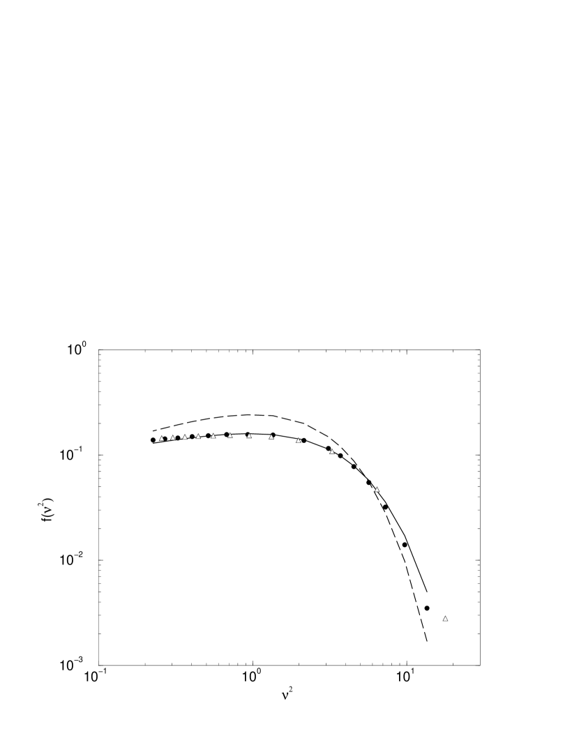
Figure 1: Comparison of the mass function derived from EPS model (dashed line) and the nonspherical collapse boundary (filled circles) with Sheth & Tormen’s fitting formula of N-body simulations (solid line). The opaque triangles show the mass function generated from the original nonspherical collapse boundary proposed by Chiueh & Lee (2001).

In Fig. 1 we compare the mass function derived from the $Y$-space diffusion with two other types of mass functions. The filled circles are the data of our six-dimensional random walks, the dashed line shows the EPS’s analytical prediction, and the solid line shows the Sheth & Tormen’s mass function (ST99), which has the form

$$\nu f(\nu)=2A[1+(a\nu^{2})^{-q}](\frac{a\nu^{2}}{2\pi})^{1/2}\mathrm{exp}(-\frac{a\nu^{2}}{2}),$$ (22)

where $a=0.707$, $q=0.3$ and $A=0.322$. We conclude that our results agree quite well with that of N-body simulation given by ST99 (c.f., Eq. (22)), except at very high mass regime. There are two reasons for us to retain this discrepancy at high mass. First, the statistics of very high mass halos is not well-controlled in N-body simulation. Therefore one can not reliably specify the number of such halos. Second, it is believed that the very high mass halos should follow spherical collapse process which is closer to the EPS method, and our results show this tendency. As a further comparison, we also demonstrate in Fig. 1 the mass function given by the original nonspherical collapse boundary proposed by Chiueh & Lee (2001). It is shown that the two NCB mass functions are roughly the same except that our mass function is more accurate in the intermediate mass range. Just as we have mentioned earlier, the high accuracy is necessary when one wants to derive the bias factor precisely since the bias factor is related to the small difference between the biased mass function and the unbiased mass function, an issue to be addressed in the next section.

3.2 Bias

The peak biasing was originally introduced by Kaiser (1984) to explain the clustering of Abell clusters, and the same idea has also been used to discuss whether the galaxy distribution traces the mass distribution (Bardeen et al. 1986). Despite focusing on specific bound objects, the bias parameter also reveals the spatial clustering of dark matter halos. One common definition of the bias in the Lagrangian coordinate is

$$\frac{\delta n}{n}=b\frac{\delta\rho}{\rho},$$ (23)

or

$$b(M)=\frac{n(M,\delta_{c}|\delta=\delta^{\prime})-n(M,\delta_{c}|\delta=0)}{n(M,\delta_{c}|\delta=0)\times\delta^{\prime}},$$ (24)

where $n(M,\delta_{c}|\delta)$ represents the number of bound objects with mass M which can be found in the large-scale uncollapsed region of density contrast $\delta$. The second term of the numerator on the right hand side $n(M,\delta_{c}|\delta=0)$, or named ”the unbiased mass function”, is actually the conventional mass function we have been discussing so far, and $n(M,\delta_{c}|\delta=\delta^{\prime})$ is ”the biased mass function” in the sense that it is embedded in the uncollapsed region with finite density contrast $\delta^{\prime}$. Mo & White (1996) have derived the bias factor under the limit $\delta<<\delta_{c}$, as shown in Eq. (7), and they also give another equivalent expression for the bias evaluated at a sufficiently large separation $r$:

$$\xi_{hh}(r,M)=b^{2}(M)\xi_{mm}(r),$$ (25)

where $\xi(r)$ is the two-point correlation function and the subscripts $hh$, $mm$ denote the halo-halo and matter-matter components respectively. This definition is often used to find the bias factor in N-body simulation.

In the EPS picture, one can calculate $b$ as:

$$b(M)=\frac{n(M,\delta_{c}-\delta^{\prime}|\delta=0)-n(M,\delta_{c}|\delta=0)}{n(M,\delta_{c}|\delta=0)\times\delta^{\prime}}=\frac{1}{\sigma(M)\times n(\nu)}\frac{dn(\nu)}{d\nu}=\frac{1}{\delta_{c}}\frac{d(\ln n(\nu))}{d(\ln\nu)},$$ (26)

indicating that the bias function is directly related to the derivative of mass function in the log-space. However, this simplicity is no longer valid in the NCB approach due to the additional $r$-distribution, and therefore the bias function can be another test for the goodness of the NCB. The biased mass function $n(M,\delta_{c}|\delta=\delta^{\prime})$ can still be obtained from the excursion set approach. The natural choice for the initial condition of six-dimensional random walks for the biased collapse is that $y_{1}=\delta^{\prime}$, whereas $y_{2}$ to $y_{6}$ are Gaussian distributed random numbers with the same variance equal to $\delta^{\prime}$. Comparing the biased mass function with the unbiased mass function already obtained in $\S$ 3.1, we are able to compute the bias function defined in Eq. (24).

In Fig. 2, we show the bias functions derived from our approach for three different initial power spectra of indices, $n=0,-1$, and $-2.$ The filled circles show the results of our algorithm of $Y$-space random walks. The solid curves denote the fitting formula of N-body simulation results found by Jing (1998):

$$b(M)=(\frac{0.5}{\nu^{4}}+1)^{(0.06-0.02n)}(1+\frac{\nu^{2}-1}{\delta_{c}})-1.$$ (27)

As a comparison, Fig. 2 also shows the predictions of the EPS model (MW96) and the moving-barrier model (Sheth, Mo & Tormen 2001). Although there exit statistical fluctuations in our data, the filled circles show that the bias function generated from the nonspherical collapse boundary is quite reasonable and has a similar tendency as the results derived from the moving barrier model in the low-mass scale. But the curves of our results turn to coincide with the EPS prediction at high masses. This tendency is also seen in Jing’s simulations.

4 Conditional Mass Function

According to the hierarchical scenario, dark matter halos are formed through merging with comparable-size halos and accretion of small halos. All kinds of interactions between halos result in changes of gravitational potential and consequently the behavior of gas components. Therefore, merger/accretion rates are believed to play a crucial role in the galaxy formation. Observations show that merger rates increase with redshift (Carlberg et al. 1994; Yee & Ellingson 1995), despite the different definitions of the merger rate. On the other hand, the dependence of merger rates on redshifts and on environments has also been studied with N-body simulations (e.g., Gottlöber et al. 2001), and the results roughly agree with the observations. It is expected that the semi-analytical approach (e.g., EPS model and NCB model) can offer succint description for merger histories. However, we must keep in mind that the semi-analytical methods deal with only the isolated halos, discarding the information of substructures within each halo. The attempt of explaining galaxy formation inside galaxy groups or clusters with semi-analytical approaches must be modified. Despite such a limitation for the cloud-in-cloud problem, the merger-tree technique is often needed to establish merger histories in the field ( Kauffmann & White 1993; Somerville & Kolatt 1999). The merger-tree method is a Monte-Carlo method based on the conditional mass function. In the literature, EPS’s conditional mass function is often used to construct merger trees. However, the results indicate that there still exhibit discrepancies with the merger history extracted from N-body simulations, which is thought to be caused mainly by the EPS model rather than the specific features of merger trees (Somerville et al. 2000). Therefore, in this section, we use the NCB model to generate a new conditional mass function with the six-dimensional random walk procedure and derive a fitting formula for it.

4.1 Construction of conditional mass function

There are two scenarios, the active picture and the passive picture, to represent the diffusion process for epochs earlier than the present. The former is with a fixed collapse boundary and let the variance of some particular mass grow with time. The latter is just the opposite which fixes the variance of mass $M$ and lowers the collapse boundary with increasing time. In order to simulate the merging problem, we adopt the second picture for simplicity. For a given redshift $z$, the collapse boundary condition can be rewritten as

$$\frac{\delta}{\delta_{c}(z)}=(1+\frac{1}{\beta_{1}}(\frac{r}{\delta_{c}(z)/\delta_{c}(z=0)})^{4})^{\beta_{2}},(\beta_{1}=0.26,\beta_{2}=0.159)$$ (28)

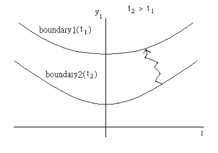
Figure 3: The nonspherical collapse boundaries of two different epochs. The higher the boundary is, the earlier the collapse time.

where $\delta_{c}(z)$ denotes the vertex of the boundary at redshift $z$ and $\delta_{c}(z=0)$ is just $\delta_{c}$ given in Eq. (18). The evolution of $\delta_{c}(z)$ is inversely proportional to the growth factor of the variance $\sigma$. For example, $\delta_{c}(z)\propto(1+z)$ in $S$CDM model. As shown in the Fig. 3, boundary 1 corresponds to the collapse condition at a time earlier than boundary 2. That is, Eq. (28) is nothing but to say that boundary 1 should be stretched both in $r$ and $\delta$ axes relative to boundary 2 to preserve the self-similar evolution of fluctuations. After collecting the trajectories that start from the origin and collapse at boundary 2 , we continue the random walks until they hit boundary1 and are absorbed.

Let $f(S_{1},\delta_{c}(z_{1})|S_{2},\delta_{c}(z_{2}))$ denote the fraction of trajectories hitting boundary 1 at mass scale $S_{1}$ to the total trajectories hitting boundary 2 at mass scale $S_{2}$. The physical meaning of $f(S_{1},\delta_{c}(z_{1})|S_{2},\delta_{c}(z_{2}))$ is the probability that a point in a halo with mass scale $S_{2}$ at redshift $z_{2}$ was in a halo with mass scale $S_{1}$ at redshift $z_{1}$. As mentioned earlier, although $S$ is the variance of the density fluctuation corresponding to a specific mass range, we use it to interpret the mass scale over which the density contrast $\delta$ is smoothed. Apparently , $S_{1}$ is always larger than $S_{2}$ to ensure that the mass of halo increase with time. Moreover, due to the self-similar scaling property of the nonspherical collapse boundary, $f$ does not depend on time explicitly, but only on the ratio of the separation, namely $\delta_{c}(z_{1})/\delta_{c}(z_{2})\equiv\kappa$. The actual time evolution of the conditional mass function is hidden in the variable $\mu$ or $\mu^{\prime}$ defined below, which is a combination of mass and time. Therefore, by simulating random walks with a particular chosen $z_{2}=0$, we are able to construct the conditional mass function which can also be applied to any other $z_{2}$.

Recalling the Pess-Schechter’s boundary, its conditional probability is given in Eq. (6), or in a concise form,

$$\mu f(\mu)d\mu=2\times(\frac{\mu^{2}}{2\pi})^{1/2}\mathrm{exp}(-\frac{\mu^{2}}{2})d\mu,$$ (29)

where $\mu\equiv(\delta_{c}(z_{1})-\delta_{c}(z_{2}))/(S_{1}-S_{2})^{1/2}=\Delta\delta_{c}/(\Delta S)^{1/2}$. Apparently, for given $z_{1}$ and $z_{2}$, the conditional probability is a function of only the difference of the variance $S$ in EPS picture. However, the conditional probability actually depends also on the initial mass scale $S_{2}$ in our scenario. This is due to that the separation of two boundaries is $S_{2}$-dependent, as is obviously indicated in Fig. 3.

Here we simulate several conditions for different boundary separations: $\kappa=1.1$, $1.3$, $2.0$, $3.0$ and $4.0$ with $z_{2}=0$. It helps the construction of a new conditional mass function by considering the following two extreme cases: when $\kappa$ approaches unit (the two boundaries are close), the conditional mass function is expected to be close to the extend Press-Schechter’s case because the two boundaries are almost parallel and most points collapsing at the first boundary will soon collapse in few steps at the second boundary. On the other hand, when $\kappa$ is very large, points in the second boundary relative to the first boundary are like that they are located at the origin, so that the conditional mass function should behave like the Sheth and Tormen’s mass function (hereafter ST mass function). We find that our simulation data can still be fitted by the following function:

$$\mu^{{}^{\prime}}f(\mu^{{}^{\prime}})d\mu^{\prime}=2A(\kappa)(1+\frac{1}{\mu^{{}^{\prime 2q}}})(\frac{\mu^{{}^{\prime 2}}}{2\pi})^{1/2}\mathrm{exp}(-\frac{\mu^{{}^{\prime 2}}}{2})d\mu^{\prime},$$ (30)

where

$$\mu^{{}^{\prime}}\equiv\frac{[\delta_{c}(z_{1})-\delta_{c}(z_{2})]\varepsilon(S_{2},\kappa)}{(S_{1}-S_{2})^{1/2}},$$ (31)

$$A=0.322+\frac{0.178}{\kappa},$$ (32)

$$\varepsilon(S_{2},\kappa)=\varepsilon(x)=0.036x^{4}-0.309x^{3}+0.944x^{2}-1.060x+1$$ (33)

with $x\equiv(\sqrt{S_{2}}/\delta_{c}(z_{2})-0.25)/\kappa$, and $q(\kappa)$ is required to satisfy the normalization condition

$$A=\sqrt{\frac{\pi}{2}}/(\sqrt{\frac{\pi}{2}}+\frac{\Gamma[-q+\frac{1}{2}]}{2\times\frac{1}{2}^{(-q+\frac{1}{2})}}).$$ (34)

Further explanation of the fitting procedure for these fitting parameters is described in Appendix A.

The mathematical form of Eq. (30) is similar to the ST mass function, which demands $A$, $q$ to be constants. Here we extend the ST mass function to the conditional mass function and introduce $A(\kappa)$, $q(\kappa)$ and $\varepsilon(S_{2},\kappa)$ as fitting functions. The definition of $\mu^{{}^{\prime}}$ here has been so motivated to fit the probability distribution derived from random walks.

However, it has been noted that when the time interval is small, i.e., $z_{2}$ close to $z_{1}$, the concept of random walks fails to describe the merger events because the excursion set neglects the correlations between scales (Peacock & Heavens 1990, Sheth & Tormen 2002), and this explains why the conditional mass function derived from the moving-barrier in a recent report (Sheth & Tormen 2002) may not be applied to construct the merger tree. Although Eqs. (30) and (31) faithfully describe the result of our random-walk processes, in order to make the conditional mass function useful even at small time interval, we find that $\mu^{\prime}$ should be modified into

$$\mu^{\prime}\equiv\frac{[\delta_{c}(z_{1})-\delta_{c}(z_{2})]\varepsilon(S_{2},\kappa)}{(S_{1}-S_{2}-\eta\delta_{c}^{2}(z_{2}))^{1/2}}.$$ (35)

The replacement of $S_{1}(M_{1})-S_{2}(M_{2})$ by $S_{1}(M_{1})-S_{2}(M_{2})-\eta\delta_{c}^{2}(z_{2})$ means that there exists a small mass gap between parent halos and progenitor halos. This small mass gap only becomes important when the look-back time is small and becomes negligible for a large look-back time. A small positive $\eta$ serves to correlate the probability of progenitor halos to that of parent halos. We find that $\eta=0.06$ gives the best result when compared with simulations, as discussed below. Furthermore, the variance and threshold value appear as $\sqrt{S}/\delta_{c}(z_{2})$ in $\mu^{\prime}$, such that the active picture and the passive picture are consistent with each other.

4.2 Comparison with N-body simulation

In order to test whether the conditional mass function derived in the previous section is valid for describing the formation history of dark halos, we compare our conditional mass function with the results of the particle-particle/ particle-mesh simulation given by Somerville et al. (2000). This simulation is a run for the $\tau$CDM model ($\Omega=1,\Gamma=0.21,h=0.5$) with box size 170 Mpc, particle number $256^{3}$. The halos are identified by using the ’friends-of-friends’ (FOF) algorithm.

To convert the conditional mass function into the probability that a halo with mass $M_{2}$ at redshift $z_{2}$ had a progenitor in the mass range $M_{1}$ to $M_{1}+dM_{1}$ at redshift $z_{1}$, we have used (LC93)

$$\frac{dn(M_{1},z_{1}|M_{2},z_{2})}{dM_{1}}dM_{1}=\frac{M_{2}}{M_{1}}f(S_{1},\delta_{c}(z_{1})|S_{2},\delta_{c}(z_{2}))|\frac{dS_{1}}{dM_{1}}|dM_{1},$$ (36)

where

$$f(S_{1},\delta_{c}(z_{1})|S_{2},\delta_{c}(z_{2}))=f(\mu^{\prime})\frac{\partial\mu^{\prime}}{\partial S_{1}}.$$ (37)

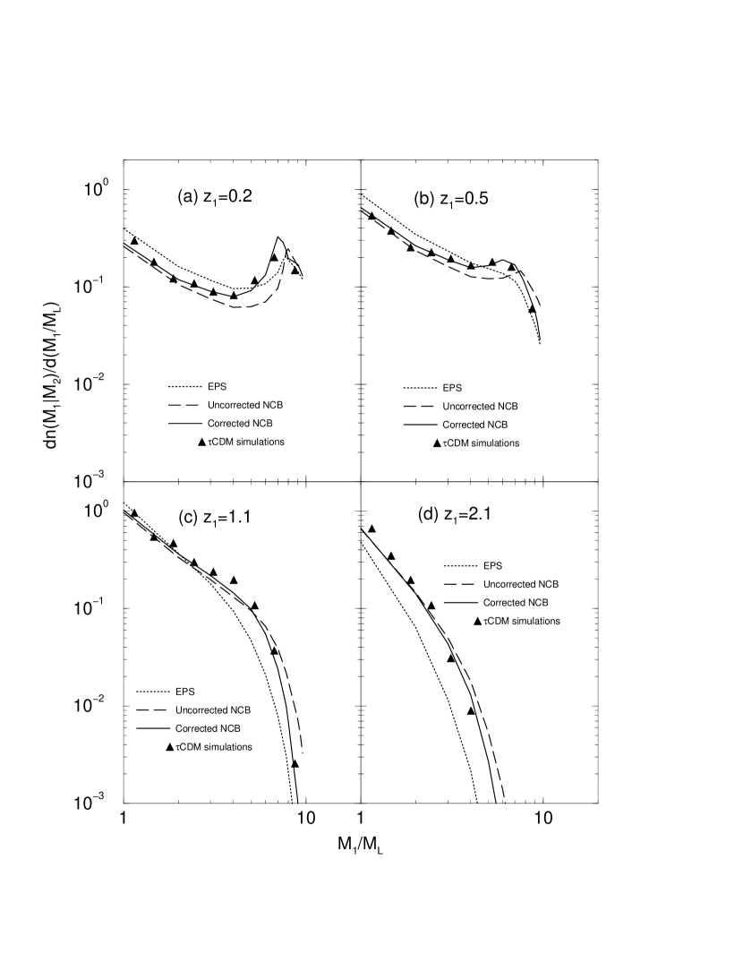
Figure 4: Comparison of the conditional mass function predicted by EPS (dotted curves), uncorrected NCB (dashed curves) and corrected NCB (solid curves) models with the results of the $\tau$CDM simulations (triangle symbols). The parent halos are chosen at $z=0$, and the progenitors are at (a) $z=0.2$, (b) $z=0.5$, (c) $z=1.1$ and (d) $z=2.1$.

The mass range of the parent halo chosen by Somerville et al. (2000) is $7.9\sim 12.6M_{L}$ at the present time ($z_{2}=0$), where $M_{L}\sim 5.0\times 10^{11}M_{\odot}$. Because the parent mass range is wide, we adopt a fair assumption that the parents of different mass obey the ST mass function. We use this distribution of $M_{2}$ to weigh the conditional mass function for the parent population. In Fig. 4, we compare the conditional mass functions predicted by our nonspherical collapse procedure and by EPS with the results of the $\tau$CDM simulation (Somerville et al., 2000). The four panels correspond to 4 different redshifts: $z_{1}=0.2,0.5,1.1$ and $2.1$. The results of $\tau$CDM simulation are represented by filled triangles; the dotted curves denote predictions of the EPS theory; the dashed curves show predictions by using Eq. (30) with the uncorrected definition of $\mu^{{}^{\prime}}$ (c.f., Eq. (31)). The solid curves, which are closer to the simulation results are our predictions with the corrected definition of $\mu^{{}^{\prime}}$ (c.f., Eq. (35)). It can be seen that introducing the small correction $\eta$ in Eq. (35) helps reproduce the conditional mass function more accurately for massive progenitor halos at small $z_{1}$. The solid curves and dashed curves can almost coincide when $z_{1}$ gets larger, as the effect of $\eta$ becomes negligible. The comparison shows that our conditional mass function (c.f., Eq. (30) & Eq. (35)) provides a better description than EPS does for a wide range of redshift. The successful description of our conditional mass function suggests that the nonspherical collapse boundary can be more ”realistic” and may be applied to construction of merger trees.

5 Conclusion

In this paper, we have attempted to show that the nonspherical collapse boundary (NCB) reproduces the mass function, bias factor and conditional mass function better than the Press-Schechter theory. This model successfully addresses these subjects over a wide range of mass scales, while the (extend) Press-Schechter theory always fails in some mass range.

Through the simulations of 6-dimensional random walks, we have shown that the bias function generated by NCB agrees with the N-body simulations reasonably well. Because NCB is more complicated than the PS’s collapse boundary, the relation between the bias function and the conditional mass function is no longer as simple as the EPS model. Especially, the two issues are not of identical representation in the framework of NCB model. We provide a formula for the conditional mass function of the nonspherical collapse boundary, which can be applied to any two redshifts. In order to overcome the problem that random-walks fail to describe the merger history at small look-back time, we add a minor correction in the definition of variable $\mu^{\prime}$ (c.f. Eq. (35)) while maintaining the overall mathematical form intact. This formula can describe the conditional mass probability more accurately than the EPS formalism over a wide mass range, even when the two epochs are close. All the results we obtained from NCB suggest that NCB is sufficiently reasonable to reproduce the statistical properties of dark halos.

There are two interesting issues pertinent to NCB: one is its natural association with the halo angular momentum through its dependence on the quantity $r$. The halo angular momentum distribution predicted by the NCB model is reported elsewhere (Chiueh, Lee and Lin, in preparation). Second, as mentioned in $\S$ 4, the conditional mass function offers an useful tool to construct the merger history through merger trees. Recent works have indicated that the merger history constructed by using EPS’s conditional mass function deviates from that extracted from N-body simulations, and it is thought to be caused mainly by the spherical-symmetry assumption of the EPS model rather than the specific features of the merger tree scheme. Thus, we expect the agreement can be greatly improved by the NCB conditional mass function given in this work.

Appendix A The fitting procedure of conditional mass function

After performing the random walks between two collapse boundaries, which are mentioned in $\S$ 4.1, we use the mathematical form of ST mass function and tune the values of A, q and $\varepsilon$ to adjust our results of random walks. It should be emphasized that A and q are not tuned independently because the integral of the function $f(\mu^{{}^{\prime}})$ should be normalized to unity, due to the assumption that all the trajectories starting from the first boundary will eventually hit the second boundary. Thus, we have

$$\int f(\mu^{{}^{\prime}})d\mu^{{}^{\prime}}=\int 2A(\kappa)(1+\frac{1}{\mu^{{}^{\prime 2q}}})(\frac{1}{2\pi})^{1/2}\mathrm{exp}(-\frac{\mu^{{}^{\prime 2}}}{2})d\mu^{\prime}=1,$$ (A1)

then we get

$$A=\sqrt{\frac{\pi}{2}}/(\sqrt{\frac{\pi}{2}}+\frac{\Gamma[-q+\frac{1}{2}]}{2\times\frac{1}{2}^{(-q+\frac{1}{2})}}).$$ (A2)

In addition, it is expected that all three parameters $A$, $q$ and $\varepsilon$ should yield a fitting formula of conditional probability to match the two extreme cases, as mentioned in $\S$ 4.1. For $\kappa$ approaching unit, i.e, the two boundaries are very close, $A(\kappa)$ gives the value $\frac{1}{2}$, and q is thus zero, which agrees with the Press-Schechter’s conditional probability. For $\kappa$ to be very large, $A$ and $q$ approach 0.322 and 0.3 respectively, the values given by Sheth & Tormen (1999). The results of our 6-dimensional simulation and our fitting formula Eq. (30) and (31) are shown in Fig. 5 $\sim$ Fig. 9. The five figures correspond to different separations of boundaries, i.e., $\kappa=1.1,1.3,2.0,3.0$, and $4.0$. The top panel of each figure is the result for initial mass scale $\sqrt{S_{2}}=0.7$, the middle panel is for $\sqrt{S_{2}}=1.5$ (around $M^{*}$) and the bottom is for $\sqrt{S_{2}}=2.9$. The opaque circles represent the data from 6-dimensional simulation and the solid lines are the best fit using Eq. (30) and (31).

We find that for the case $\kappa$ is fixed, $A$ does not vary with the initial mass scale $S_{2}$, i.e., $A$ is a function of $\kappa$ only. In Fig. 10, we show the relation between $A$ and $1/\kappa$. The square symbols show the fitting values of A for five different $\kappa$ plus two boundary values: $(1/\kappa,A)=(0,0.322)$ and $(1,0.5)$, which recover the limit conditions associated with EPS and ST cases. The solid line represents here is a linear relation between $A$ and $1/\kappa$:

$$A=0.322+\frac{0.178}{\kappa},$$ (A3)

which is determined by the above two boundary points. This line almost passes through the other five fitting points and thus is a good representation for $A(\kappa)$. Combined with Eq. (A2), $q$ can be determined immediately for each $\kappa$.

Our tests also show that $\varepsilon$ is a function of a combined variable $x\equiv(\sqrt{S_{2}}/\delta_{c}(z_{2})-0.25)/\kappa$. The best fit of the function is (see Fig. 11)

$$\varepsilon(x)=0.036x^{4}-0.309x^{3}+0.944x^{2}-1.060x+1.$$ (A4)

This result is consistent with the geometry of two boundaries. Since we have the $r$-distribution of various mass scales $S_{2}$’s that hit the first boundary, one can estimate roughly the distance between two boundaries for each mass scale. It is easily seen that for a fixed $\kappa$, the gap $d$ initially decreases to reach a minimum and then rises when $S_{2}$ continues to increase. The behavior of $d/(\delta_{c}(z_{1})-\delta_{c}(z_{2}))$ agrees with that of $\varepsilon$ defined above.

Figure 2: The bias factor as a function of $M/M^{*}$ for three different initial power indices:(a) n=0, (b) n=-1 and (c) n=-2. The circle symbols show the results of our algorithm of $Y$-space random walks. The solid curves are Jing’s fitting formula derived from N-body simulations. The long dashed lines denote the analytical bias prediction based on EPS (MW96), and the dot-dashed lines show the results predicted by moving-barrier model (Sheth, Mo & Tormen 2001).

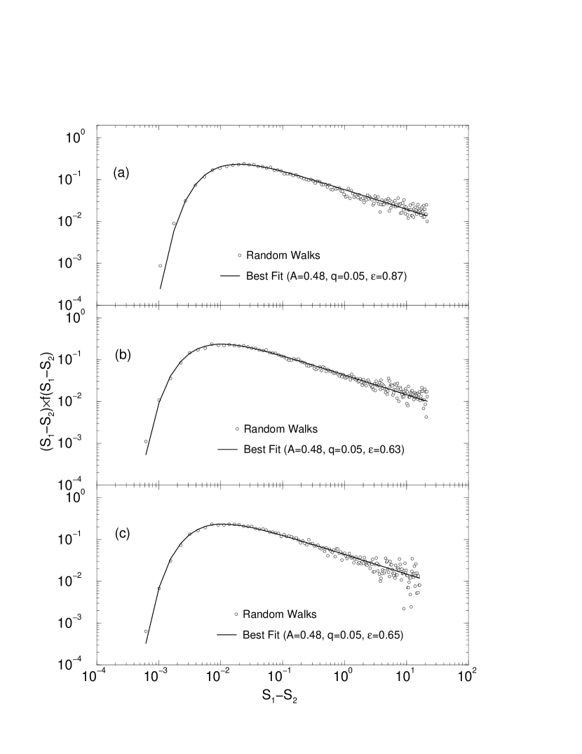
Figure 5: The conditionalmass function for $\kappa=1.1$. The opaque circles represent the results of the six-dimensional random walks and the solid lines are the best fit using Eqs. (30) and (31). The mass scale at time $z_{2}$ is chosen as (a) $\sqrt{S_{2}}=0.7$, (b) $\sqrt{S_{2}}=1.5$ and (c) $\sqrt{S_{2}}=2.9$.

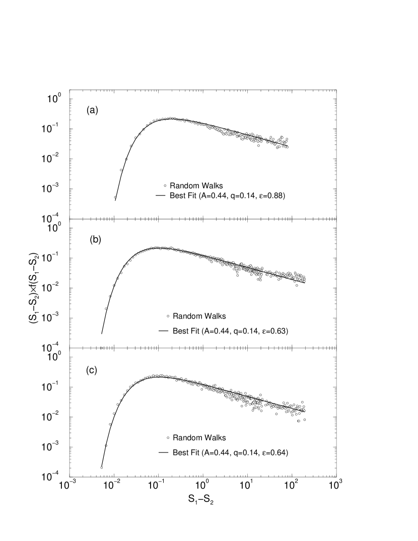
Figure 6: Same as the previous figure, but for $\kappa=1.3$.

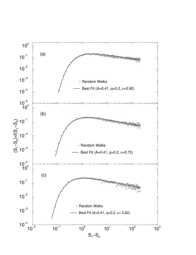
Figure 7: Same as the previous figure, but for $\kappa=2.0$.

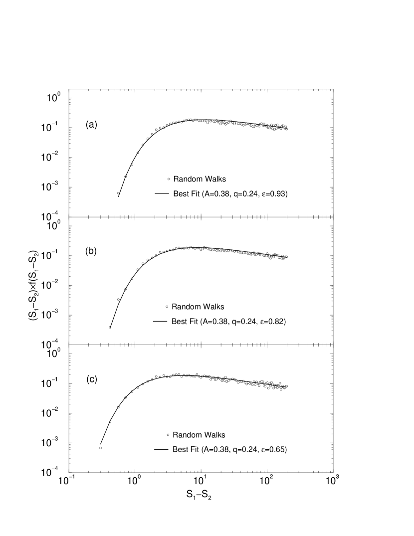
Figure 8: Same as the previous figure, but for $\kappa=3.0$.

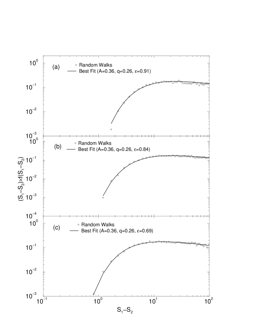
Figure 9: Same as the previous figure, but for $\kappa=4.0$.

Figure 10: $A-1/\kappa$ relation. The square symbols show the five fitting values of $A$ for our data, the filled triangle represents the EPS case, the filled circle represents the case of ST mass function, and the solid line denotes the linear relation between $A$ and $1/\kappa$ (c.f., Eq. (32)).

Figure 11: $\varepsilon$ factor as a function of $x(\equiv(\sqrt{S_{2}}/\delta_{c}(z_{2})-0.25)/\kappa)$. Similar to Fig. 10, the square symbols show the fitting values of $\varepsilon$ for our data and the solid line denotes the fitting relation of the square symbols (c.f., Eq. (33)).

References

- Bardeen et al. (1986) Bardeen, J. M., Bond, J. R., Kaiser, N., & Szalay, A. S. 1986, ApJ, 304, 15
- Bond et al. (1991) Bond, J.R., Cole, S., Efstathiou, G., & Kaiser, N. 1991, ApJ, 379, 440
- Bond & Myers (1996) Bond, J. R. & Myers, S. T. 1996, ApJS, 103, 1
- Bower (1991) Bower, R. G. 1991, MNRAS, 248, 332
- Carlberg et al. (1994) Carlberg, R. G., Protchet, C. J., & Infante, L. 1994, ApJ, 435, 540
- Catelan & Theuns (1996) Catelan, P., & Theuns, T. 1996, MNRAS, 282, 436
- Chiueh & Lee (2001) Chiueh, T., & Lee, J. 2001, ApJ, 555, 83 .
- Chandrasekhar (1943) Chandrasekhar, S. 1943, Rev. Mod. Phys., 15, 2
- Efstathiou (1988) Efstathiou, G., Frenk, C. S., White, S. D. M., & Davis, M. 1988, MNRAS, 235, 715
- Gottlöber et al. (2001) Gottlöber, S., Klypin, A., & Kravtsov, A. V. 2001, ApJ, 546, 233
- Jing (1998) Jing, Y. P. 1998, ApJ, 503, L9
- Kaiser (1984) Kaiser, N. 1984, ApJ, 284, L9
- Kauffmann & White (1993) Kauffmann, G., & White, S. D. M. 1993, MNRAS, 264, 201
- Lacey & Cole (1993) Lacey, C., & Cole, S. 1993, MNRAS, 262, 627
- Lacey & Cole (1994) Lacey, C., & Cole, S. 1994, MNRAS, 271, 676
- Lee & Shandarin (1998) Lee, J., & Shandarin, S. F. 1998, ApJ, 500, 14.
- Mo & White (1996) Mo, H. J., & White, S. D. M. 1996, MNRAS, 282, 347
- Monaco (1995) Monaco, P. 1995, ApJ, 447, 23
- Peacock & Heavens (1990) Peacock, J. A., & Heavens, A. F. 1990, MNRAS, 243, 133
- Press & Schechter (1974) Press, W., & Schechter, P. 1974, ApJ, 187, 425
- Shapiro et al. (1999) Shapiro, P. R., Iliev, I., & Raga, A. C. 1999, MNRAS, 307, 203
- Sheth & Tormen (1999) Sheth, R. K., & Tormen, G. 1999, MNRAS, 308, 119
- Sheth et al. (2001) Sheth, R. K., Mo, H. J., & Tormen, G. 2001, MNRAS, 323, 1
- Sheth & Tormen (2002) Sheth, R. K., & Tormen, G. 2002, MNRAS, 329, 61
- Somerville & Kolatt (1999) Somerville, R. S., & Kolatt, T. 1999, MNRAS, 305, 1
- Somerville et al. (2000) Somerville, R. S. et al. 2000, MNRAS, 316, 479
- Yee & Ellingson (1995) Yee, H. K. C., & Ellingson, E. 1995, ApJ, 445, 37
- Zeldovich (1970) Zeldovich, Ya. B. 1970, A&A, 5, 84