Performance and Simulation of the RICE detector

Abstract

The RICE experiment (Radio Ice Cherenkov Experiment) at the South Pole, co-deployed with the AMANDA experiment, seeks to detect ultra-high energy (UHE) electron neutrinos interacting in cold polar ice. Such interactions produce electromagnetic showers, which emit radio-frequency Cherenkov radiation. We describe the experimental apparatus and the procedures used to measure the neutrino flux.

I Ultra-High Energy Neutrino Astronomy: Introduction

Detection of ultra-high energy ($E_{\nu}>10^{15}$eV) neutrinos represents a unique opportunity to probe the distant universe. High-energy protons and photons from distant sources are likely to interact with the cosmic microwave background (CMB); protons, being charged, have their trajectories bent in galactic and intergalactic magnetic fields. Neutrinos are inert to CMB photons and point directly back to their source, giving essential information on those sources. In the realm of particle physics, detection of UHE neutrinos from cosmological distances, if accompanied by flavor identification, may permit measurement of neutrino oscillation parameters over an unprecedented range of $\Delta m^{2}$. It has been suggested that, with a sensitive enough array, tau neutrinos may be identified by two-step “double-bang”[1] processes where a $\tau$ lepton is created and subsequently decays. Since neutrino absorption in the earth depends on the chord length through the earth, the angular distribution of detected neutrino events could be used to verify predictions for weak cross-sections at energies unattainable by any man-made accelerator. Alternately, if the high energy weak cross-sections are known, they can be used to test Earth composition models along an arbitrary chord (‘neutrino tomography’)[2].

A Current Experimental Efforts

Several recent projects (including AMANDA[3], NESTOR[4], Lake Baikal[5], ANTARES[6]) are optimized for detection of very high energy ($10^{12-15}$ eV) cosmic ray muon neutrinos. Sensitivities to higher energies, as well as electromagnetic cascades, have also been shown to be substantial in such experiments[7, 8]. These instruments are based on photomultiplier tube detection of the optical Cherenkov cone from muons produced in muon neutrino charged current interactions. At high energies, muons have ranges of order 1 km and follow approximately straight trajectories (smeared by multiple scattering), punctuated by catastrophic bremstrahlung every 0.1–1 km or so, in which $\sim$10% of the muon’s energy is lost to a photon. RICE employs radio detection, which is believed to be the most efficient detection mechanism at energies of $10^{15}$ eV and beyond[9].

FIG. 1.: Simulated RICE event. The actual detector geometry is shown, to scale.

The RICE concept is illustrated in Figure 1, depicting a Cherenkov cone fit to a set of “struck” dipole receivers in a simulation event, along with the extracted neutrino direction. Receiver locations are drawn to scale in the Figure. In the actual array geometry, dipole receivers are spread over a 200 m $\times$ 200 m $\times$ 200 m cube beneath and around the Martin A. Pomerantz Observatory (MAPO), approximately 1 km. from the geographic South Pole.

B Radio Detection

We have initiated a pilot program based on radiowave receiver technology in order to extend electron neutrino detection up to the PeV energy scale. The detector is intended to have sensitivity in the energy range $E_{\nu_{e}}\sim 10^{15}-10^{18}$ eV. RICE (“Radio Ice Cherenkov Experiment”) should ultimately be capable of observing the sky with angular resolution of $\sim$10-50 mrad.

Coherent radio Cherenkov emission is an efficient method for detecting high energy particles. The history of the effect goes back to Jelley, who first considered whether cosmic ray air showers might produce a radio signal[10]. Askaryan[11] subsequently predicted a net charge imbalance in air showers, and coherent radio power proportional to the energy of the shower squared. Substantial radio emission from atmospheric electromagnetic cascades was observed more than 30 years ago[10, 12]. Progress in ultra-high energy air showers has sparked renewed interest, and new observations of radio pulses have been reported recently[13], suggesting a possible radio component to the Auger detector[14]. A recent international meeting highlights current progress[15].

This effect has recently been observed in a test-beam experiment at SLAC[16]. A beam of electrons, of known amperage, was fired into a sand target and the radiation resulting from the impact measured in the radio regime. As Figure 2 illustrates, the measured signal strength (diamonds) displays the expected dependence on both total beam current (left, solid curve) and frequency (right, dashed curve).

FIG. 2.: Results of testbeam experiment[14], showing signal strength and expected dependence on total beam current (circles, left) and frequency (diamonds, right). Figure reprinted courtesy of D. Saltzberg and P. Gorham.

C Initiation of the RICE Experiment

The RICE experiment was initiated in October, 1995 when the AMANDA collaboration graciously consented to co-deployment of two shallow radio receivers (“Rx”) in the first holes being drilled for AMANDA-B. Following deployment, a surface transmitter (“Tx”) was used to verify that signals could be detected under-ice with better than 10 ns timing precision. However, cross-talk and amplifier oscillation problems precluded use of those receivers for science. The first three dedicated RICE receivers were deployed in 1996-97, along with one underice transmitter. The extraordinary RF clarity of South Polar ice was amply illustrated by the evident brightness of the AMANDA photomultiplier tubes 2 km. below the RICE receivers (and close to the null in the dipole antenna’s reception pattern). A Fourier analysis of the RF transients produced by AMANDA photo-tubes in laboratory conditions indicated that PMT background power dominated at frequencies below 100 MHz, motivating use of high-pass filters in subsequent Rx deployments. Antenna deployments followed in 1997-98 (three more receivers and two more transmitters deployed in AMANDA-B holes), 1998-99 (six receivers deployed in 5”-diameter dedicated RICE holes, bored using a mechanical, rather than a hot-water drill), and 1999-2000 (six receivers, and one transmitter deployed in AMANDA-B holes).

II Experimental Apparatus

The RICE experiment presently consists of an 18-channel array of radio receivers (“Rx”), scattered within a 200 m$\times$200 m$\times$200 m cube, at 100-300 m depths. Each receiver contains a half-wave dipole antenna, offering good reception over the range 0.2–1 GHz. Twelve receivers are buried in the boreholes drilled for the AMANDA photomultiplier tube deployment during the 1996-97, 97-98, and 99-00 austral summers. Six receivers are located in dedicated RICE holes; four such holes were drilled with a 5-inch diameter mechanical hole-borer in 1998-99. The signal from each antenna is immediately boosted by a 36-dB in-ice amplifier, then carried by $\sim$300 m coaxial cable to the surface observatory, where the signal is filtered (suppressing noise below 200 MHz due to both AMANDA photo-tubes, as well as continuous wave backgrounds from South Pole station at 149 MHz), re-amplified (either 52- or 60-dB gain), and split into two copies. One copy is fed into a CAMAC crate from which, after initial discrimination (using a LeCroy 3412 discriminator), the signal is routed into a NIM crate where the trigger logic resides. The other copy of the analog signal from the antennas is input to one channel of a digital oscilloscope, where waveform information is recorded. Also deployed are three large TEM surface horn antennas which are used as a veto of surface-generated noise.

A Detector Array Status

The status of the current array deployment is summarized in Figure 3.

FIG. 3.: Present geometry of the RICE array, relative to AMANDA hole 4. “Tx” designate transmitters; “Rx” designate receivers. Depths of receivers, as well as relative cable diameter (indicated by the thickness of horizontal lines before the antenna identifier), is also indicated.

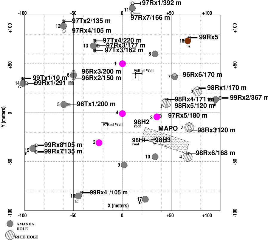
Indicated in the Figure are the AMANDA holes (1-19, drilled using the hot-water technique) containing RICE receivers, and also the four holes drilled specifically for RICE in 1998-99 containing RICE-only equipment. All channels are indicated by a 5-character alphanumeric mnemonic corresponding to the year of deployment, the type of dipole antenna deployed (transmitter “Tx” or receiver “Rx”; these only differ by the installation of a receiver amplifier in the latter modules), and a numerical identifier. Also indicated in the Figure is the MAPO building which houses hardware for several experiments, including the RICE and AMANDA surface electronics. The AMANDA array is located approximately 600 m (AMANDA-A) to 1400 m (AMANDA-B) below the RICE array in the ice; the South Pole Air Shower Experiment (SPASE) is located on the surface at $x\sim-400$m in the Figure. The coordinate system conforms to the convention used by the AMANDA experiment; grid North coincides with the +y-direction in the Figure.

B Event Trigger and Vetoes

The main RICE trigger condition requires that four or more channels have their output voltage exceed a common adjustable threshold within a pre-set time window (currently $\Delta t=1.2\mu$s, set by the radio wave transit time across the array). The threshold is adjusted so that thermal fluctuations, or other backgrounds, do not cause excessive triggers. The time window allows for coincidences across the full array, independent of event geometry. A valid event trigger is also defined when, in a time window of 1.2 $\mu$s, i) $\geq$ one underice antenna registers a signal above threshold in coincidence with a 30-fold PMT AMANDA-B trigger, or: ii) $\geq$ one underice antenna registers a signal above threshold in coincidence with a high-multiplicity SPASE event.

Additionally, there are two ways that surface-generated background transient events can be vetoed – either: a) one of the surface horn antennas registers a signal above threshold, in which case data-taking is inhibited for the subsequent 4 $\mu$sec, or b) the timing sequence of hits in the underice antennas is determined to be consistent (in software) with the sequence expected from surface-generated backgrounds. This “surface-veto” algorithm uses the time differences between TDC hits recorded on-line to make a fast ($<$10 msec) classification of the event as surface/non-surface in origin. One of every 10000 events classified as “surface” (i.e., having a sequence of antenna hits consistent with a $Z>$0 vertex) are retained to ensure that this veto is functioning properly.

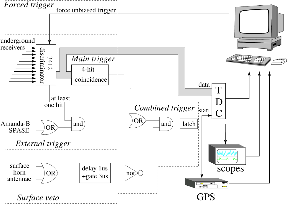
If any of the above trigger criteria are satisfied and there is no veto signal, the time of each hit above threshold (as recorded by a LeCroy 3377 TDC), and also an 8.192 $\mu$s buffer of data stored in an HP54542 digital oscilloscope at 1 GSa/s (for each channel) is written to disk. Each event is also given a GPS time stamp for synchronization with other South Pole (and more global) experiments. To monitor the stability of the amplifiers as well as changing background conditions, waveform measurements are taken every ten minutes, independent of other event triggers (so-called “unbiased” triggers). A schematic of the event trigger is shown in Figure 4.

FIG. 4.: Functional schematic of RICE event trigger.

1 Discriminator Efficiency

As the first element in the event trigger, it is essential that the Lecroy 3140 Discriminator module operates efficiently for nanosecond duration pulses. The discriminator efficiency is checked explicitly in the lab using an 800 ps width signal (generated by an HP8133A signal generator) fed directly into a 3140 Discriminator module, and also verified in the field by pulsing the array with a 600 ps width signal broadcast through one of the broadband TEM horns (the bandwidth of the horns is $\sim$3 GHz, so timing is preserved down to $\sim$300 ps). The LeCroy discriminator is found to be $>$99% efficient in triggering on the narrowest width pulses our signal generator is capable of producing. Given the measured impedances of our cable, amplifiers, and antennas (discussed below), a neutrino pulse is expected to produce signals of width $\sim$1-3 ns[17] at the surface.

C Raw Data

Raw trigger rates (before veto) are typically 30 Hz; data-taking rates after the veto are typically 0.01 – 0.1 Hz. The data-taking rate (and, correspondingly, our experimental livetime) is limited by: a) the time required to write information from the digital oscilloscopes to disk ($\sim$10 sec/event), b) the time required to perform the surface-background veto in software ($\sim$10 msec/event), and c) our inability to take data at those times when the South Pole satellite uplink (broadcast at 303 MHz) is active, due to the high amplitude of the uplink signal. When this uplink is not active, the discriminator thresholds correspond to typical livetimes of $\sim$80%. Based on known dead times in the system, integrated array on-time is currently monitored and updated on-line.

A typical event, as recorded in the HP54542A oscilloscopes, is shown in Figure 5.

FIG. 5.: Typical data event recorded by the RICE array (Feb. 11, 1999). This event was vetoed as having a surface origin, based on the observed sequence of hit times (see text).

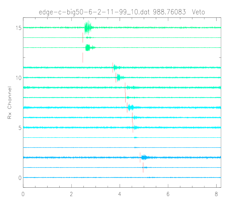
In the event display, each of the 8.912 $\mu$sec traces corresponds to one of the under-ice antennas. Vertical bars indicate the TDC time recorded for each particular channel. Note that one channel (12) has no waveform information, and two channels are not used in the trigger (13 and 15) and therefore have no TDC information. Also note that channels which do not have hits which exceed the initial discriminator threshold do not register a TDC time. The rise time and leading-edge timing resolution of each receiver as determined by waveform information can be approximately estimated from the Figure. The leading edge resolution is typically 2 nsec; the ring time for each antenna is typically tens of nanoseconds. In the Figure, the antennas have been ordered according to their distance from the surface, with the shallowest (/deepest) antennas at the top (/bottom) of the Figure. The pattern of hits shown is therefore easily identifiable as a surface-generated RF pulse sweeping down through the radio array.

The Fourier transform of a typical waveform signal (channel 7) is displayed in Figure 6. The general shape of the signal in the frequency domain reveals many interesting features of the experimental hardware and the environment. Below 200 MHz, suppression of noise due to the filter is evident; as mentioned previously, use of this filter was motivated by the need to reduce low-frequency RF backgrounds due to broadband galactic sky noise, monochromatic Continuous Wave (CW) sources at the Pole, as well as the firing of AMANDA phototubes. Above 200 MHz, losses due to cable effects become increasingly pronounced. At the time this event was recorded, the 303 MHz satellite uplink at the Pole was active; the peak at this frequency is evident in this Fourier Transform.

FIG. 6.: Fourier transform of raw data waveform corresponding to channel 7 of the previous Figure. The South Pole station satellite uplink at 303 MHz is evident in the Figure. A high pass filter suppresses signals below $\sim$180 MHz. Other features of this distribution are discussed in the text. No corrections for cable loss, signal amplification, etc. have been made. (The vertical scale is arbitrary.)

III Timing Calibration

Event and source reconstruction is based on our knowledge of the array geometry, ice properties and thus the expected times for a wave-front to propagate from the source to any given receiver location. A time-of-hit is defined as the time of the first excursion exceeding $6\sigma_{rms}$ in a waveform; $\sigma_{rms}$ is determined from the sample of “unbiased” events which are taken every 600 seconds, independent of the event trigger status. The maximum resolution on the hit-times cannot, therefore, exceed the sampling time of the oscilloscopes (1 ns). This resolution can be improved using a “matched filter” algorithm which matches the observed waveform with a reference signal waveform; such a software algorithm is currently under development. In the “matched filter” approach, one defines a reference signal corresponding to the expected damped oscillator response of the antenna to an impulsive signal: $f(t)\sim e^{-Rt/L}cos(\omega t)$, with $\omega=\sqrt{1/RC}$. The values of $R$, $L$ and $C$ can be estimated from network analyzer measurements of the complex antenna impedance ${\vec{Z}}_{antenna}$ (described below), as a function of frequency. The signal time is defined as that time which maximizes the integral: $\int f(t)V(t)dt$, with $V(t)$ given by the direct data measurement of the waveform voltage with time. As an illustration of the potential improvement arising from the matched filter algorithm, Figure 7 compares the raw signal $V(t)$ (top panels) with the output of the filter algorithm (lower panels) for one channel (channel 2) in one event. The signal to noise is clearly superior in the latter case.

FIG. 7.: Raw V(t) for two waveforms (top); the signal time as determined by a simple maximum voltage algorithm corresponds to the maximum excursion from zero. Bottom displays show the quantity $\Sigma f(t)V(t)$, with $f(t)$ being the damped oscillator reference signal and $V(t)$ the actual recorded waveform shown in top panels. The signal to noise is clearly greater for the filter output.

Knowing the time differences $\delta t_{ij}$ between all pairs $(i,j)$ of hit antennas, we perform $\chi^{2}$ minimization to find a source location. Once the vertex location has been found, superimposing a Cherenkov cone of half-width 57^∘ on the hit antennas allows a determination of the source direction. For the full reconstruction, this method requires at least four antennas to be hit (i.e., 3$\delta t_{ij}$ values). Uncertainties in $\delta t_{ij}$ arise from several sources, including risetime resolutions ($\sim$2 ns), differences in signal propagation velocity in the ice due to variations in the dielectric constant with depth, differences in signal propagation speed within the different analog cables being used, differences in cable lengths, and receiver deployment surveying uncertainties.

Buried transmitters (“Tx”) are used to calibrate the channel-to-channel timing delays. A short duration pulse is sent to one of the five under-ice transmitters, which subsequently broadcasts the signal to the receiver array. An event vertex is reconstructed exclusively from the measured channel-to-channel time delays; constraining the source to a unique location allows a calculation of the timing residual $\chi^{2}$ for each channel, based on the timing uncertainty: $\chi^{2}_{t}(ij)=({\delta t_{ij}^{\rm measured}-\delta t_{ij}^{\rm expected}\over\sigma_{t}(ij)})^{2}$. An iterative procedure is used to calibrate out the observed channel-to-channel timing delays and minimize the timing residuals for an ensemble of events. Typical timing calibration corrections are $\sim$10 ns per channel; these corrections are then used for all subsequent event reconstruction.

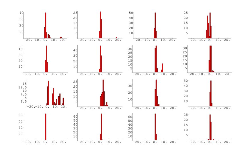
Once the source location has been determined, the timing resolution for each channel can be derived by examining the width of the $(\delta t_{ij}^{\rm measured}-\delta t_{ij}^{\rm expected})$ distribution. After time calibrations have been performed, these differences of time differences should (ideally) be zero for a unique vertex. Figure 8 shows these distributions, with channel 12 (arbitrarily) chosen as the reference channel. From these plots, the signal arrival time resolution for good channels (i.e., all channels except channel 8 in the Figure) is determined to be $\sim$1.5–2 ns, slightly larger than the oscilloscope sampling time of 1 ns.

FIG. 8.: Time difference between calibration signal arrival time in ch. i relative to ch. 12, in nanoseconds. Data taken from transmitter pulser event sample. Oscilloscope jitter in channel 8 is evident from the distributions.

A Vertex Reconstruction Algorithms

Two algorithms are used to determine a source location. The first, a “trial-and-error” procedure, tests the consistency of each possible (x,y,z) source location, in a grid 2km x 2km x 1km below and around the radio array, with the observed data. I.e., the $(xgrid,ygrid,zgrid)$ source point (using a step size of 10 m, or a total of $4\times 10^{6}$ source points tested) corresponding to the minimum $\chi^{2}$ is identified. The advantage of this procedure is that time distortion effects due to ray tracing through regions with varying index of refraction can easily be incorporated; the disadvantage is speed and the intrinsic dependence on the grid spacing. The second procedure analytically determines the source location ${\vec{r}_{source}}$ and a global event time $t_{0}$ by simultaneous solution of the 4 equations: $|r_{Rx,i}-r_{source}|=(c/n)t_{i}$ ($i=1,2,3,4$), where $r_{Rx,i}$ is the vector from the origin to receiver $i$, $r_{source}$ is the vector from the origin to the source, and $t_{i}$ is the hit time recorded for the $i^{th}$ receiver. There are at most two roots: eliminating complex or acausal roots, while also requiring consistency of 5 or more hits resolves ambiguities. In Cartesian coordinates, we denote this analytic solution for the source location as ${\vec{r}}_{source}$=$(x4hit,y4hit,z4hit)$.

FIG. 9.: Reconstruction of Tx pulse from transmitter 97Tx2, based exclusively on measured receiver times. 4-hit solutions are shown as the unshaded histogram; grid solutions to the vertex location are shown as the shaded histogram.

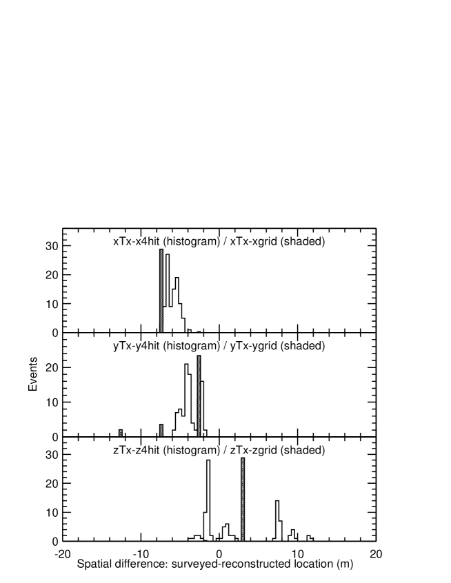
Source reconstruction results are shown in Figure 9. Three plots, each showing the difference between the reconstructed vertex location and the surveyed vertex location in one of the spatial coordinates, are shown. Based on the (general) consistency between both the 4-hit and the grid algorithms with the surveyed Tx location, we conclude that the surveying error in the Tx location is less than 5 m.

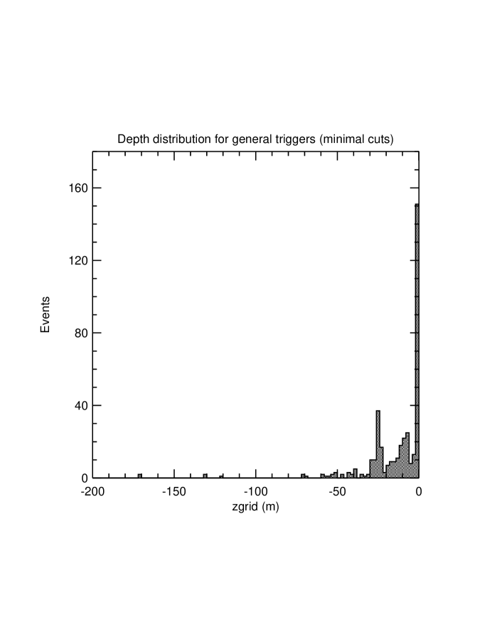
For general events (such as those displayed in Figure 5), we expect backgrounds generated at the surface to dominate. Figure 10 shows the reconstructed source depth ($zgrid$) for a sample of general triggers; as expected, sources populate the region above the array.

FIG. 10.: Typical depth distribution for a sample of 348 general RICE triggers. Triggers are observed to be dominated by sources near the surface. (There are no underflow entries.)

B Dielectric Constant of Ice

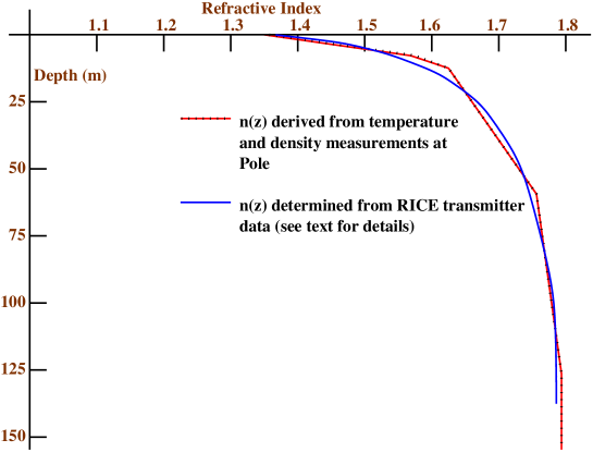
The complex dielectric constant ${\epsilon}(\omega)$ allows one to calculate both the absorptive and refractive effects of the ice. The imaginary part of the dielectric constant (related to the “loss tangent”) prescribes losses due to absorption; the real part corresponds to the refractive index of the medium. Information on the refractive index can be derived from temperature and density profiles, as a function of depth, acquired by AMANDA deep drilling operations. Such profiles ($z(T,\rho)$) can be combined with laboratory measurements of the dependence of the index of refraction of ice on temperature and density ($n(T,\rho)$) to predict the expected index of refraction profile at the South Pole as a function of depth $n(z)$. This derived $n(z)$ function can be compared with the profile calculated directly from RICE transmitter data. Using the surveyed transmitter and receiver locations, combined with Fermat’s principle, one can determine the profile $n(z)$ which best reproduces the observed $Tx\to Rx$ radio signal transit times. A preliminary comparison between the measured $n(z)$ function determined from transmitter data with the “derived” $n(z)$ profile is shown in Figure 11. Agreement is satisfactory; however, work is still in progress to quantify the agreement between the two curves.

FIG. 11.: Index of refraction as a function of depth.

Absorption of radio waves in cold glacial ice is temperature, density, and frequency dependent and has been measured [18], indicating attenuation lengths $\alpha\sim$1-10 km at frequencies in the range 100 MHz – 1 GHz. Given the small scale of our current array ($\sim$100 m) compared to the very large attenuation length $\alpha$ expected for Polar ice in the 100 MHz – 1 GHz regime, our transmitter tests are consistent with zero absorption over our short baseline; long baseline transmitter measurements are an objective of future Polar campaigns.

IV Antenna Response and Gain Calibration

To detect a neutrino of a given energy interacting at a given distance from an antenna, we need to quantify the sensitivity of the array to the resulting Cherenkov signal. Although neutrino vertex location reconstruction is based only on channel-to-channel timing, an amplitude calibration is needed in order to ensure that the discriminator efficiency, for a given incident neutrino energy, is reliably calculable.

A Antenna Effective Area

One of the fundamental parameters used to define the power response of an antenna is the effective area $A_{eff}(\theta,\phi)$ (or gain $G=4\pi A_{eff}/\lambda^{2}$); this is related to the incident signal intensity $I$ as: $P_{out}=IA_{eff}$. We have used two techniques to measure the effective area $A_{eff}$ of RICE dipole antennas. The first applies the Friis Transformation Equation to data taken when a transmitter (Tx) broadcasts to a receiver (Rx) on the KU Antenna Testing Range (KUATR). The Friis Equation relates the power broadcast by the transmitter to the signal intensity measured at the Rx (valid in the far-field case). Defining the monochromatic power into the transmitter $P_{Tx,in}$, the power broadcast outwards from the transmitter $P_{Tx,out}$, the power intercepted by the receiver $P_{Rx,in}$, and the power transmitted out the back of the receiver: $P_{Rx,out}$ (which we measure either on an oscilloscope or a network analyzer), we have: $P_{Tx,out}=P_{Tx,in}G_{Tx}$, $I_{Rx,in}=P_{Tx,out}/(4\pi R^{2})$, $P_{Rx,out}=I_{Rx,in}A_{eff,Rx}=P_{Tx,out}A_{eff,Rx}/(4\pi R^{2})$; ${P_{Rx,out}\over P_{Tx,in}}=G_{Tx}A_{eff,Rx}/(4\pi R^{2})$. Using a calibrated transmitter, $G_{Tx}$ is known; by comparing to a calibrated receiver ($A_{eff,Rx}^{standard}$ known), the gain or effective area of any arbitrary antenna can be inferred by a simple ratio.

Alternately, the gain/effective area can be determined by sending a known amount of power through a cable and into an antenna. The reflection coefficient $\Gamma_{R}$ (having real and imaginary components $\Gamma_{r}$ and $\Gamma_{i}$, respectively) measures the impedance mismatch of the antenna ${vecZ}_{antenna}$ and the cable $Z_{cable}$, and is ideally zero for a high-gain antenna (impedance well-matched to 50$\Omega$ cable, e.g.). Numerically, $G\sim(1-|\Gamma_{R}|^{2})$. The two measurements of $A_{eff}$ (from the testing range and the impedance measurement, respectively) agree to within $\pm$1 dB over the frequency range of interest and are consistent with simple expectations for dipoles.

B Effective Height

To understand the shape of the signal voltage produced by a receiver in the time domain, we must quantify the complex effective height ${\vec{h}}$[19]. The effective height ${\vec{h}}$ (in units of meters) is related to the magnitude and the phase of the voltage resulting from the application of a complex electric field vector at the antenna load by: $V_{out}={\vec{E}_{in}}\cdot{\vec{h}}$ = $h{\vec{E}_{in}}\cdot{\hat{n}_{A}}$. The effective area and the magnitude of the effective height can be related through: $|{\vec{h}}|\sim\sqrt{A_{eff}/(120\pi)}$ $=\sqrt{\lambda^{2}(Gain)/(480\pi^{2})}$. The polarization of ${\vec{h}}$ is aligned along the dipole axis ${\hat{n}}_{A}$ as ${\vec{h}}=h{\hat{n}}_{A}$, where $|h|$ is the magnitude of effective height.

The full, complex transfer function ${\vec{T}}(\omega)$ for the antenna, in principle, gives a complete description of the antenna (+cable) response and can be related to the effective height. This function ${\vec{T}}(\omega)$ can be written as the product of the complex impedance of the (antenna+cable) ${\vec{Z}}(\omega)$ multiplied by the complex height function ${\vec{h}}(\omega)$, properly taking into account potential mismatches between the impedance of the antenna and the impedance of the attached cable: ${\vec{T}}={\vec{h}}(Z_{cable})/({\vec{Z}_{antenna}}+Z_{cable})$, with $Z_{cable}$=50$\Omega$+$i0\Omega$. Both the magnitude and phase of the effective height are determined directly from KUATR measurements. ${\vec{Z}_{antenna}}$ is determined from reflected power measurements on a HP8713C Network Analyzer (NWA). An independent check on the internal consistency of our ${\vec{Z}}_{antenna}$ determinations is presented in Appendix 1.

The magnitude of the effective height measured for a typical RICE dipole is given in Figure 12. The peak frequency in air ($\sim$600 MHz)

FIG. 12.: Modulus of RICE dipole effective height (m.) as a function of frequency. Shown are data taken on the KU antenna testing range, with a Fourier fit overlaid.

is roughly consistent with the dimensions of the half-dipole ($\sim$15 cm); the effective height, as expected, also has magnitude of order 10 cm. at the peak frequency.

The phase variation of the effective height has also been measured as a function of frequency at KUATR and found to be negligible (put another way, we find that, to a very good approximation the experimental slope of the phase variation with frequency is linear: $\Delta\phi(\phi)\approx 0.031\phi$ (rad). Such a linear variation has no net effect on overall antenna response.). Given the magnitude of the effective height, the phase variation of the effective height, and therefore the magnitude and phase variation of the complex antenna impedance ${\vec{Z}}(\omega)$, the complex transfer function ${\vec{T}}(\omega)$ can now be calculated, and used to predict the expected waveform $V^{\prime}(t)$ observed in a RICE antenna in response to a transmitter signal. This is done by transforming the input impulse $V(t)$ to frequency space, multiplying the function $V(\omega)$ by the transfer function ${\vec{T}}(\omega)$ for both Tx and Rx (properly normalized), and then transforming back to the time domain to give $V^{\prime}(t)$. Figure 13 shows the result of this exercise. Qualitatively, the after-pulsing observed in data is reproduced by our complex transfer function. We note that the actual expected signal shape observed for a neutrino event requires knowledge of the details of the input signal, as discussed in the references[20, 21].

FIG. 13.: Expectation for observed RICE receiver signal shape $V^{\prime}(t)$ based on measured effective height and complex impedance function, given a short duration input signal to a RICE transmitter.

Dipole response has also been measured as a function of both azimuthal and polar angles. The polar angle response is observed to be well approximated by a $cos^{2}\theta$ dependence (in power); the dipole response in azimuth is observed to be flat, as expected.

C Amplifier Gain Calibration

Signals from the antennas are boosted by two stages of amplification, totaling between +88 dB and +96 dB of gain, depending on the channel. For a RICE waveform containing only (“unbiased”) thermal noise, the total power in a frequency bandwidth $B$ can be calculated from the discrete Fourier transform of the waveform as $P_{noise}=kTB$ (we check several 50 MHz-wide frequency bins from 250 to 500 MHz for this calculation). Since the total noise power in this band at the input to the antenna can also be written as a sum over the rms voltage measured in each frequency bin: $P_{<V>}=\Sigma_{\omega}{V_{\omega}^{2}\over Z}$, we can also write $P_{<V>}=P_{noise}G$, where $G$ is the overall gain of the system. Thus, based on the rms voltage $<V>$ of the 8192 samples contained in these “unbiased” waveforms, the gain of the amplifiers can be calculated in situ. The amplifier gain measured this way is flat up to the bandwidth limit of the oscilloscopes (500 MHz); direct laboratory measurements of the amplifier gain using a network analyzer are consistent with flat response up to 750 MHz. Most($>$90%) of the amplifiers are stable to 1-2 dB over the course of data-taking thus far analyzed.

D Full Circuit Amplitude Calibration

FIG. 14.: Comparison of expected (solid curve) vs. measured (histogram) Tx$\to$Rx signal strength for one transmitter broadcasting to 16 receivers. Vertical scale is Return-Power/Transmit-Power, in dB. No data is shown for the receiver (channel 2, top row) in the same hole as the transmitter being used for this test, due to possible cross-talk effects. Corrections for the measured roll-off of surface amplifier gain for some channels above 700 MHz have been only approximated.

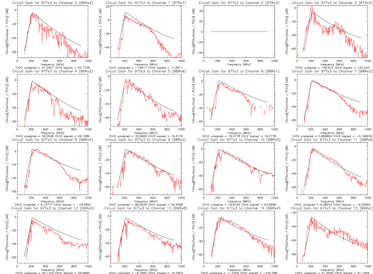
In the final step of our amplitude calibration, the antenna response to a continuous wave (CW) signal broadcast from an under-ice transmitter is measured in situ. This test calibrates the combined effects of all cables, signal splitters, amplifiers, etc. in the array. A 1 milliwatt (0 dBm) continuous wave signal is broadcast through the transmit port of an HP8713C NWA. The NWA scans through the frequency range 0$\to$1000 MHz in 1000 bins, producing a 0 dBm CW signal in each frequency bin. The signal is transmitted down through $\sim$1000 feet of coaxial cable to one of the five under-ice dipole transmitting antennas. The transmitters subsequently broadcast this signal to the under-ice receiver array, and the return signal power from each of the receivers (after amplification, passing upwards through receiver cable and fed back into the return port of the NWA) is then measured. Using laboratory measurements made at KUATR of: a) the effective height of the dipole antennas, as a function of frequency (previously described), b) the dipole Tx/Rx efficiency as a function of polar angle and azimuth, c) cable losses and dispersive effects (cables are observed to be non-dispersive for the lengths of cable, and over the frequency range used in this experiment), d) the gain of the two stages of amplification as determined from RICE data acquired in situ by normalizing to thermal noise $P_{noise}=kTB=\Sigma_{\omega}<V_{ant}^{2}>/Z$, summing over all frequency bins, and e) finally correcting for $1/r^{2}$ spherical spreading of the signal power, one can model the receiver array and calculate the expected signal strength returning to the input port of the network analyzer. This can then be directly compared with actual measurement. Such a comparison, as a function of frequency, is shown in Figure 14 for one transmitter (97Tx3). Below 200 MHz, the attenuating effect of the high-pass filter is evident. From the Figure, agreement is observed to be $\sim$3-6 dB (in power) for the full circuit gain. Note that no correction for ice absorption has been made, given the small scale of the array.

Similarly, for each frequency bin we can calculate the difference between calculated vs. measured full-circuit gain. Figure 15 shows the deviation between the calculated gain minus the measured gain, for several data runs. Included in the Figure are each of the 500 one MHz bins between 200 MHz and 700 MHz, for three transmitters. This Figure therefore shows the average deviation between model and measurement over that frequency range; for the five currently functional transmitters, the mean differences between the expected and the measured gain are $-0.6\pm 0.6$, $-0.8\pm 0.6$, $-2.3\pm 0.5$, $-3.4\pm 0.6$ and $-2.8\pm 0.6$ dB.

FIG. 15.: Deviation between expected vs. measured Tx$\to$Rx signal power for three transmitters broadcasting to 16 receivers.

Within the “analysis” frequency band of our experiment (200 MHz - 500 MHz), our quoted level of uncertainty in the total receiver circuit power is $\pm$6 dB; this value is commensurate with the width of the gain deviation distributions. On average, however, the calculated gains quoted above are well within these limits. Note also that, for all of the transmitters, the measured gain is actually higher than expected. To calculate eventual upper limits on the neutrino flux, however, we will use the more conservative calculated full-circuit gain.

V Monte Carlo simulation of detector performance

In order to check our understanding of the timing and gain calibrations of our experiment, we have written a Monte Carlo simulation of the RICE array. This simulation allows us to study the expected response of the radio receiver array to either a Cherenkov signal (as generated by a true $\nu_{e}N\to eN^{\prime}$ charged-current event) or a random noise coincidence such as those expected to dominate our backgrounds. The simulation also checks our expected timing resolution (2 ns, as determined by measuring the channel-to-channel residuals for pulsed transmitter events in data) as well as study the effects of the overall gain uncertainty discussed previously (6 dB per channel, max, obtained by examining the residuals between calculated vs. measured gain for continuous wave signals from 200-700 MHz). Expected vertex (spatial) and angular (pointing) resolution, as well as neutrino energy resolution can, in principle, be assessed with the simulation.

A Monte Carlo Event Generation

Neutrino interactions are generated uniformly in incident angle, with vertices uniformly populating the region: $|x|<$1 km, $|y|<$1 km and $0<z<$1 km. After specifying a source location and incident neutrino energy, the simulation generates receiver times (smeared by our timing uncertainty of $\sim$2 ns) and voltages at the input to the antenna, based on GEANT simulations of radio signals in ice[21]. In addition to the voltage due to the neutrino interaction, thermal noise is also simulated at the input to the antenna. Antenna response, as a function of frequency, is modeled as described above; knowing the amplifier gain and cable losses, the voltage recorded at the surface is calculated, and smeared by the gain uncertainty of $\pm$6 dB ($\pm$3 dB in voltage). With simulated times and simulated voltages, simulated events are then reconstructed with the same software used for data.

B Checks of the Simulation - MC vs. Data Tx Depth Reconstruction

As a first check of the simulation, we have compared reconstructed transmitter source depths in data vs. Monte Carlo simulations. The source locations reconstructed from data collected when a pulser was connected to transmitter 97Tx3 were compared to 97Tx3 simulations, as shown in Figure 16. Vertices are reconstructed using the analytic 4-hit technique described previously. The simulation adequately reproduces both the location (to within 1 m) as well as the width of the source distribution.

FIG. 16.: Comparison between reconstructed depth of transmitter (97Tx3), from pulser data taken at the South Pole, and Monte Carlo simulations of 97Tx3 pulser events. Times are smeared in the simulation by a Gaussian of width 2 ns.

C Expected Vertex Depth Resolution Dependence on Depth

As a further example of the utility of the simulation, Figure 17 shows the expected vertex depth resolution (essential in discriminating surface sources from in-ice sources), as a function of the true source depth. Not unexpectedly, the resolution is best when the source vertex is close to the array and the event geometry is best resolved. Deep sources are increasingly difficult to pinpoint; additionally, the reconstruction software tends to reconstruct source vertices that are closer than the actual source ($z_{reconstructed}-z_{true}<$0); i.e., vertices tend to be pulled closer to the array. This bias is under study.

FIG. 17.: Deviation between reconstructed and true interaction depth ($z4hit$), vs. true interaction depth, from Monte Carlo simulations. The reconstructed vertex here was obtained using the analytic, 4-hit vertexing algorithm. The size of the squares corresponds to the number of reconstructed events in the Monte Carlo simulation.

D Angular Resolution

Good angular resolution is essential in discriminating up-coming from down-going sources. Additionally, some physics analyses (e.g., coincidences with Gamma-Ray Bursts) are limited by the ability to point back to the recorded sky location of the GRB. For neutrinos that interact very far from the array, the angular resolution is expected to be poor – the further the source point, the greater the inability to measure the Cherenkov wavefront, and the more the array “looks” like a single space-point relative to the interaction point. Figure 18 displays the angular resolution for an ensemble of 10 PeV neutrinos interacting within 1 km in the ice below the array; we have required that at least four of the simulated receiver voltages exceed threshold and can therefore be used in vertex reconstruction. For approximately half the events, the angular resolution is about 10 degrees. The long tail in this distribution is due to distant source points which have correspondingly poorer pointing resolution.

FIG. 18.: Monte Carlo prediction for RICE array angular resolution, in units of degrees. Events ($E_{\nu}=$10 PeV) have been simulated over the region within 1 km below and around the current array.

E Energy Resolution

Having reconstructed a vertex location, the distance from each antenna to that vertex is determined. Having reconstructed the event geometry (i.e., the Cherenkov cone fit), we know the angular deviation of each antenna off the cone. The greater this angular deviation, the weaker the antenna signal strength. Finally, given the voltages recorded on each antenna, we have enough information to make an estimate of the incident neutrino energy. For each antenna, the inferred value of $E_{\nu}$ is calculated; we define $E_{\nu,reconstructed}$ as the simple average of the $E_{\nu}$ estimates obtained from each antenna. Fig. 19 shows the expected energy resolution ($log_{10}(E_{\nu,reconstructed}/E_{\nu,generated})$) for 10 PeV neutrinos generated uniformly over distances within 1 km of the array. The resolution is obviously superior in cases where the hit antenna multiplicity is large ($N_{hit}>$10) vs. cases where the hit multiplicity is small.

FIG. 19.: Histogram of number of events vs. logarithm (base 10) of Reconstructed/true neutrino energy, as obtained from neutrino interaction simulations. The sample is divided into high hit multiplicities ($>$10) and low hit multiplicities ($\leq$10). The energy resolution is obviously better for events with higher hit multiplicities. The simulated event sample is the same as that of the previous Figure.

F Conical vs. Spherical Source Event Geometries

Perhaps most important in discriminating background from true neutrino-induced events is the characteristic conical Cherenkov distribution of energy in the latter case. Background (from the surface, e.g.) typically consists of spherical waves due to transient sources. We measure the consistency of a given event with either a conical or a spherical source by a “trial-and-error” procedure similar to the “grid”-based vertex-finding algorithm: given a reconstructed source location, we find the Cherenkov cone orientation most consistent (in terms of a minimum $\chi^{2}_{cone}$ variable) with the observed channel-to-channel voltages. Spherical sources should therefore correspond to large values of $\chi^{2}_{cone}$ since a conical source would typically have a smaller number of large-voltage signals than a spherical source. This is illustrated in Figure 20, where we compare the $\chi^{2}_{cone}$ distribution for: a) general, 4-hit RICE triggers, taken from data, b) calibration pulser events, taken from data, c) Monte Carlo simulations of a pulser source (97Tx3) emitting spherical waves, and d) Monte Carlo simulations of neutrino events producing Cherenkov cones. The separation between conical vs. spherical source geometries is evident from the Figure, as well as the rough agreement between data and the simulation of a spherical source near the array.

FIG. 20.: $log_{10}(\chi^{2})$ of fit of recorded voltages (for both data and simulation) for spherical vs. conical geometry sources. The separation between conical and spherical sources, as well as the agreement between simulation and data for spherical sources, is evident from the Figure.

VI Summary

Basic calibration of both the time and amplitude response of RICE radio receivers has been made, relying primarily on data taken in situ. A Monte Carlo simulation has been written which reproduces the gross features of those calibration data. The calibration of the detector is sufficient to allow limits to be placed on the incident high-energy neutrino flux.

APPENDIX 1: Check of Antenna Impedance

We can check the internal consistency of our ${\vec{Z}_{antenna}}$ measurements by constructing an appropriate Green function to give the antenna response to a given input. Impedance is, in effect, a Green function - namely, an analytic function in the complex $\omega$ plane, reflecting the constraint of causality in the time domain.

The Zeroes and Poles Expansion of the impedance of a network implements the essential analytic features. It states: The impedance of a network containing any number of $L,\,R,\,C$ elements, including antennas, is a rational function of $\omega$, which can always be factored into simple zeroes and poles[22]:

$$Z(\omega)=\frac{(\omega-\omega_{0})(\omega-\omega_{1})(\omega-\omega_{2})..}{i\omega(\omega-\omega^{\prime}_{0})(\omega-\omega^{\prime}_{1})(\omega-\omega^{\prime}_{2})...}.$$ (1)

The expansion follows from the definition $Z(\omega)=V(\omega)/I(\omega)$ and the expansion of $V(\omega)$ and $I(\omega)$ into polynomial ratios, which can be factored. The pole at $\omega=0$ is just the static capacitance of the device. The poles and zeroes are symmetric about the imaginary axis and all lie in the lower $\omega$ half-plane, consistent with causality.

Since all the poles and zeroes are simple and isolated, an equivalent ansatz is a sum of familiar “Breit-Wigner” resonances,

$$iZ(\omega)=\sum_{J}\frac{-i\alpha_{J}\omega\omega_{J}}{\omega^{2}-\omega_{J}^{2}+i\Gamma_{J}\omega}.$$ (2)

Here $\omega_{J}$ is the value of a resonant antenna frequency, and $\Gamma_{J}$ is the width; the constant $\alpha_{J}$ measures the strength.

Check of impedance ansatz with data

A Hewlett-Packard network analyzer HP8712C measured real and imaginary reflection coefficients $\Gamma_{r},\,\Gamma_{i}$ for antennas in the lab. Tests were made after calibrating out cable, connector and lead effects. The reflection coefficients are related to the complex impedance $Z(\omega)$ by

$$Re(Z(\omega))={1-\Gamma_{r}^{2}-\Gamma_{i}^{2}\over(1-\Gamma_{r})^{2}+\Gamma_{i}^{2}}~{}{\rm and}~{}Im(Z(\omega))={2\Gamma_{i}\over(1-\Gamma_{r})^{2}+\Gamma_{i}^{2}}.$$ (3)

Variations from antenna to antenna were observed to be small, typically 10% or less and considered smaller than other variables in the calibration chain.

Figure 21 shows the real and imaginary parts of the antenna impedance measurements over the approximate range $50MHz-5GHz$. This range substantially exceeds the range over which the antenna impedance needs to be known, due to cutoffs at the low and high frequency ends from the high-pass filter and cable losses, respectively. These effects are well-characterized and discussed elsewhere. The Figure shows real and imaginary parts as “bumps” and wiggle-excursions consistent with Breit-Wigner physics.

We tested our understanding of the antennas by fitting the real part (only) of the impedance to a sum of Breit Wigner functions. This is straightforward because the resonant frequency is located near the bump maximum and the width can be estimated from the graphs. Fitting one-half of the data is the same procedure as fitting a dispersion relation, namely

$$iZ(\omega)=\frac{1}{2\pi i}\int_{-\infty}^{+\infty}d\omega^{\prime}\,\frac{Im(iZ(\omega^{\prime}))}{\omega-\omega^{\prime}}.$$ (4)

Compared to standard dispersion relations, real and imaginary conventions are reversed in impedance, with the absorptive part of impedance (resonant bumps) defined as real-valued.

Once the real part was fit, it was used to predict the imaginary part of the impedance (Fig. 21, gray lines). The predictions agree with the data and serve as a check of the entire procedure.

FIG. 21.: Real (positive only) and imaginary (both positive and negative values) antenna impedance data obtained from network analyzer measurements (dots), as a function of frequency (MHz). The vertical scale is linear and in absolute units of 50 ohms. After performing a multiple Breit-Wigner fit to the real part of the impedance function $Re(Z(\omega))$, the imaginary part of the impedance is predicted directly from the real part by the dispersion relation. Agreement between the calculated and the measured values of $Im(Z)$ is satisfactory.

REFERENCES

- [1] J. Learned and S. Pakvasa, hep-ph/9408296
- [2] A. Nicolaidis (Thessaloniki U.), M. Jannane, A. Tarantola (Paris, Curie Univ. VI, Inst. Phys. Globe), preprint THES-TP-90-03, Jul 1990.; P. Jain, J. P. Ralston and G. Frichter, Astroparticle Physics 12, 193 (1999). See also J. P. Ralston, in 26th International Cosmic Ray Conference (Salt lake City 1999) edited by D. Kieda and B. L. Dingus (IUPAP 1999).
- [3] E. Andres et al. Astropart Phys, 13 (2000) 1.
- [4] See Proc. of 3rd NESTOR Intl. Workshop, Ed. L.K. Resvanis, Athens, Greece, Univ. Press, 1993
- [5] V. Balkanov et al., astro-ph/0001151, to appear in the Proceedings of International Conference on Non-Accelerator New Physics, June 28 - July 3, 1999, Dubna, Russia
- [6] F. Montanet, astro-ph/0001380, Talk given at TAUP99, the Sixth International Workshop on Topics in Astroparticle and Underground Physics, College de France, Paris, France, September 6-10, 1999
- [7] Monte Carlo simulations have shown that the implementation of Transient Waveform Recorders (TRW’s), planned by the AMANDA collaboration for use in 2002, should significantly improve sensitivity to electromagnetic cascades in the ice.
- [8] The AMANDA Collaboration, “Search for Neutrino Induced Cascades with the AMANDA-B10 Detector” in Proc. of the 26th Intl. Cosmic Ray Conference, DESY, Zeuthen, Germany (2001)
- [9] Price, P. B., astro-ph/951011, (1995), and Astropart. Phys. 5, 43, (1996).
- [10] Allan, H. R., Progress in Elementary Particles and Cosmic Ray Physics, North-Holland Publishing Company, Amsterdam, 1971.
- [11] Askaryan, G. A., Zh. Eksp. Teor. Fiz. 41,616 (1961) [Soviet Physics JETP 14, 441 (1962)].
- [12] Jelley, J. V. et al, Nu. Cim. X46, 649 (1966)
- [13] Rosner, J. L. and Wilkerson, J. F., EFI-97-10 (1997), hep-ex/9702008; Rosner, J. L., DOE-ER-40561-221 (1995), hep-ex/9508011. Rosner, J. L., Extensive Air Shower Radio Detection: Recent Results and Outlook, astro-ph/0101089 invited talk presented by J. Rosner at RADHEP-2000 Conference, Nov. 16-18, 2000 (UCLA).
- [14] M. Ave et al., astro-ph/0003011
- [15] See, e.g., Proc. of the 1st International Workshop on Radio Detection of High-Energy Particles (RADHEP-2000), Nov 16-18, 2000 (UCLA).
- [16] D. Saltzberg et. al., Phys. Rev. Lett.
- [17] Frichter, G. M., Ralston J. P., and McKay, D. W., Phys. Rev. D 53, 1684 (1996).
- [18] V. V. Bogorodsky and V. P. Gavrilo, Ice: Physical Properties, Modern Methods of Glaciology (Lenningrad, 1980); V. V. Bogorodsky, C. R. Bentley and P. E. Gundmandsen, ”Radioglaciology”, Reidel Publishing (1985).
- [19] C. W. Harrison and C. S. Williams, IEEE Trans. Anten. Prop., AP-13, 236 (1965)
- [20] Zas, E., Halzen, F., and Stanev, T., Phys. Rev. D 45, 362 (1992).
- [21] S. Razzaque et. al., in preparation, and S. Razzaque et. al., in the Proc. of the 1st International Workshop on Radio Detection of High-Energy Particles (RADHEP-2000), Nov 16-18, 2000 (UCLA).
- [22] S. A. Shellkunoff and H. T. Friis, Antennas: Theory and Practice, (Wiley, New York, 1952); and S. A. Shellkunoff , Advanced Antenna Theory, (Wiley, New York, 1952).