Scaling of ISM Turbulence: Implications for HI

Abstract

Galactic HI is a gas that is coupled to magnetic field because of its fractional ionization. Many properties of HI are affected by turbulence. Recently, there has been a significant breakthrough on the theory of magnetohydrodynamic (MHD) turbulence. For the first time in the history of the subject we have a scaling model that is supported by numerical simulations. We review recent progress in studies of both incompressible and compressible turbulence. We also discuss the new regime of MHD turbulence that happens below the scale at which conventional turbulent motions get damped by viscosity. The viscosity in the case of HI is being produced by neutrals and truncates the turbulent cascade at parsec scales. We show that below this scale magnetic fluctuations with a shallow spectrum persist and point out to a possibility of the resumption of the MHD cascade after ions and neutrals decouple. We discuss the implications of the new insight into MHD turbulence for cosmic ray transport and grain dynamics.

475 N. Charter St., Department of Astronomy, Univ. of Wisconsin, Madison, WI53706, USA; cho, lazarian, & yan@astro.wisc.edu

1. Introduction

The interstellar medium (ISM) is clumpy and turbulent (Larson 1981; Myers 1983; Scalo 1987; see also Lazarian, Pogosyan & Esquivel, this volume, henceforth LPE02) with an embedded magnetic field that influences almost all of its properties. This turbulence that ranges from AUs to kpc (Armstrong et al. 1995, Stanimirovic & Lazarian 2001, Deshpande et al. 2000) holds the key to many astrophysical processes (e.g., star formation, fragmentation of molecular clouds, heat and cosmic ray transport, magnetic reconnection).

All turbulent systems have one thing in common: they have large “Reynolds number” ($Re\equiv LV/\nu$; L=characteristic size of the system, V=velocity different over this size, and $\nu$=viscosity), the ratio of the time required for viscous forces to slow it appreciably ($L^{2}/\nu$) to the eddy turnover time of a parcel of gas ($L/V$). A similar parameter, the “magnetic Reynolds number”, $Rm$ ($\equiv LV/\eta$; $\eta$=magnetic diffusion), is the ratio of the magnetic field decay time ($L^{2}/\eta$) to the eddy turnover time ($L/V$). The properties of the flows on all scales depend on $Re$ and $Rm$. Flows with $Re<100$ are laminar; chaotic structures develop gradually as $Re$ increases, and those with $Re\sim 10^{3}$ are appreciably less chaotic than those with $Re\sim 10^{7}$. Observed features such as star forming clouds are very chaotic with $Re>10^{8}$ and $Rm>10^{16}$.

Let us start by considering incompressible hydrodynamic turbulence, which can be described by the Kolmogorov theory (Kolmogorov 1941). Suppose that we excite fluid motions at a scale $L$. We call this scale the energy injection scale or the largest energy containing eddy scale. For instance, an obstacle in a flow excites motions on the scale of the order of its size. Then the energy injected at the scale $L$ cascades to progressively smaller and smaller scales at a rate of eddies turning over, i.e. $\tau_{l}^{-1}\approx v_{l}/l$, with the energy losses along the cascade being negligible. Ultimately, the energy reaches the molecular dissipation scale $l_{d}$, i.e. the scale where the local $Re\sim 1$, and is dissipated there. The scales between $L$ and $l_{d}$ are called the inertial range and it typically covers many decades. The motions over the inertial range are self-similar and this provides tremendous advantages for theoretical description.

The beauty of the Kolmogorov theory that it does provide a simple scaling for hydrodynamic motions. If the velocity at a scale $l$ from the inertial range is $v_{l}$, the Kolmogorov theory states that the kinetic energy ($\rho v_{l}^{2}\sim v_{l}^{2}$ as the density is constant) is transferred to next scale within one eddy turnover time ($l/v_{l}$). Thus within the Kolmogorov theory the energy transfer rate ($v_{l}^{2}/(l/v_{l})$) is scale-independent, and we get the famous Kolmogorov scaling     $v_{l}\propto l^{1/3}$   .

One-dimensional energy spectrum $E(k)$ is one of the most important quantities in turbulence theories. Note that $E(k)dk$ is the amount of energy between the wavenumber $k$ and $k+dk$. When $E(k)$ follows a power law, $kE(k)$ is the energy near the wavenumber $k\propto 1/l$. Since $v_{l}^{2}$ represents a similar energy, $v_{l}^{2}\approx kE(k)$. Therefore, Kolmogorov scaling entails       $E(k)\propto k^{-5/3}$   .

Kolmogorov scalings constitute probably the major advance of the microscopic turbulence theory of incompressible fluids. They allowed numerous applications in different branches of science (see Monin & Yaglom 1975). However, astrophysical fluids are magnetized and the application of the Kolmogorov scalings is not easy to justify. For instance, dynamically important magnetic field should interfere with eddies motions.

Paradoxically, astrophysical measurements reveal the Kolmogorov spectra (see LPE02). For instance, interstellar scintillation observations indicate electron density spectrum follows a power law over 7 decades of length scales (see Armstrong et al. 1995). The slope of the spectrum is very close to $-5/3$ for $10^{6}m$ - $10^{14}m$. At larger scales LPE02 summarizes the evidence of $-5/3$ velocity power spectrum over pc-scales in HI. Solar-wind observations provide in-situ measurements of the power spectrum of magnetic fluctuations and Leamon et al. (1998) also obtained a slope of $\approx-5/3$. Is this a coincidence? What properties the magnetized compressible ISM is expected to have? These sort of questions we will deal with below.

Here we describe our approach which is complementary to that in Vazquez-Semadeni (this volume). The latter attempts to simulate the ISM in its complexity by including many physical processes (e.g. compression, self-gravity) simultaneously. As a downside of this, such simulations cannot distinguish between the consequences of different processes. We discuss a focused approach when only after obtaining clear understanding on the simplest level, the next level is attempted. Therefore, we first consider incompressible MHD turbulence (§2), then discuss the viscous damping of incompressible turbulence in §3, and then we consider the effect of compression in §4. We discuss implications of our new understanding of MHD turbulence for the problems of dust motion and cosmic ray scattering in §5.

2. Incompressible MHD Turbulence

2.1. Theory

Observations suggest that the random component of magnetic field is comparable with the regular component. Therefore, we consider the case that the rms velocity at the energy injection scale is comparable to the Alfven speed of the mean field. This means that we do not deal with the problem of magnetic field generation, or magnetic dynamo (see Kulsrud & Anderson 1992; Vishniac & Cho 2001; Maron & Cowley 2001).

An ingenious model very similar in its beauty and simplicity to the Kolmogorov one has been proposed by Goldreich & Sridhar (1995; hereinafter GS95) for incompressible MHD turbulence. Earlier theories by Iroshnikov (1963) and Kraichnan (1965) did not account for the anisotropy created by magnetic field. In GS95, however, it is noted that the motions mixing magnetic field lines happen essentially hydrodynamically and therefore the energy transfer rate is roughly $\tau_{nl}^{-1}\approx k_{\bot}v_{k}$ where $k_{\bot}$ is the wavevector component perpendicular to the local magnetic field. These mixing motions in the GS95 model are coupled with the wave-like motions parallel to magnetic field which results in critical balance condition    $k_{\|}V_{A}\sim k_{\bot}v_{k}$    , where $k_{\|}$ is the component of the wavevector parallel to the local magnetic field.

Conservation of energy in the turbulent cascade implies that the energy cascade rate $\dot{\epsilon}$ ($=v_{l}^{2}/\tau_{nl}$) is constant:

$$\dot{\epsilon}\sim\frac{v_{k}^{2}}{\tau_{nl}}=\mbox{constant.}$$ (1)

Combining this with the critical balance condition we obtain an anisotropy that increases with the decrease of the scale     $k_{\|}\propto k_{\perp}^{2/3}$    , and a Kolmogorov-like spectrum for perpendicular motions

$$v_{k}\propto k_{\perp}^{-1/3},\mbox{~{}~{}or,~{}}E(k)\propto k_{\perp}^{-5/3},$$ (2)

which is not surprising as magnetic field does not influence motions that do not bend it. At the same time, the scale-dependent anisotropy reflects the fact that it is more difficult for weaker small eddies to bend magnetic field.

GS95 shows the duality of turbulent motions. Those perpendicular to magnetic field are essentially eddies, while those parallel to magnetic field are waves. The critical balance condition couples the two types of motions.

2.2. Numerical simulations

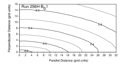
(a)	(b)
(c)	(d)

Figure 1.: (a) Velocity correlation function (VCF) from a simulation. Contours represent shape of different size eddies. The smaller contours (or, eddies) are more elongated. (b) VCF generated from equation (3). (c) Semi-major axis and semi-minor axis of contours of the same VCF (as in Fig. 1a). See Cho & Vishniac (2000) for details. (d) Cross-sections of (a part of) the data cube Fourier components $k>20$. Darker tones represent stronger magnetic field strength. The direction of the mean field is marked by an arrow. Magnetic fields show elongated structures along the mean field ${\bf B}_{0}$ (bottom of the cube). No systematic structures exist in the perpendicular plane (back side of the cube). Figures by Cho, Lazarian, & Vishniac.

Numerical simulations by Cho & Vishniac (2000) and Maron & Goldreich (2001) have confirmed GS95 theory, e.g. the Kolmogorov-type scaling and the scale-dependent anisotropy ($k_{\|}\propto k_{\perp}^{2/3}$), and helped to extend it. The important point that escaped earlier researchers was that the scale dependent anisotropy can be measured only in a local coordinate frame which is aligned with the locally averaged magnetic field direction (see Cho & Vishniac 2000). Further research in Cho, Lazarian, & Vishniac (2002a: hereinafter CLV02a) certified that in the local system of reference the mixing motions perpendicular to magnetic field are identical to hydrodynamic motions (compare Müller & Biskamp 2000).

Fig. 1 illustrates some of our results. The contours of the equal correlation obtained in Cho & Vishniac (2000) are shown in Fig. 1a and are consistent with the predictions of the GS95 model. Fig. 1c. shows that the semi-major axis ($1/k_{\|}$) is proportional to the 2/3 power of the semi-minor axis ($1/k_{\perp}$), implying that $k_{\|}\propto k_{\perp}^{2/3}$. While one dimensional energy spectrum follows Kolmogorov spectrum, $E(k)\propto k^{-5/3}$, CLV02a showed that 3D energy spectrum is

$$P(k_{\perp},k_{\|})=(B_{0}/L^{1/3})k_{\perp}^{-10/3}\exp\left(-L^{1/3}\frac{k_{\|}}{k_{\perp}^{2/3}}\right),$$ (3)

where $B_{0}$ is the strength of the mean field and $L$ is the scale of the energy injection. Velocity correlation from the 3D spectrum provides an excellent fit to the numerical data (Fig. 1b). This allows practical applications illustrated in §5.

All in all, it has been shown that the magnetized incompressible turbulence is both similar and dissimilar to the Kolmogorov turbulence. If we consider motions perpendicular to magnetic field, they are hydrodynamic-like. This entails the Kolmogorov-type spectrum reported by many observers. However, unlike Kolmogorov turbulence, the magnetized one is anisotropic with the degree of anisotropy increasing with the decrease of the scale. This entails much of a difference and requires substantial revisions of many earlier calculations.

2.3. Decay of turbulence

Turbulence plays a critical role in molecular cloud support and star formation and the issue of the time scale of turbulent decay is vital for understanding these processes. If MHD turbulence decays quickly, then serious problems face the researchers attempting to explain important observational facts, e.g. turbulent motions seen within molecular clouds without star formation (Myers 1999) and rates of star formation (Mckee 1999). Earlier studies attributed the rapid decay of turbulence to compressibility effects (Mac Low 1999). GS95 predicts and numerical simulations, e.g. CLV02a, confirm that turbulence decays rapidly even in the incompressible limit. This can be understood if mixing motions perpendicular to magnetic field lines are considered. As we discussed earlier, such eddies, as in hydrodynamic turbulence, decay in one eddy turnover time.

Below we consider the effect of imbalance on the turbulence decay time scale. Duality of the MHD turbulence means that the turbulence can be described by opposite-traveling wave packets. ‘Imbalance’ means that wave packets traveling in one direction have significantly larger amplitudes than those traveling in the other direction. In the ISM, many energy sources are localized both in space and time. For example, in terms of energy injection, stellar outflows are essentially point energy sources. With these localized energy sources, it is natural that interstellar turbulence be typically imbalanced.

Here we show results of the CLV02a study that demonstrates that imbalance does extend the lifetime of MHD turbulence (see Fig. 2a). We use a run on a grid of $144^{3}$ to investigate the decay time scale. We run the simulation up to t=75 with non-zero driving forces. Here $t$ is measured in the units of the large-scale eddy turnover time (L/V). Then at t=75, we turn off the driving forces and let the turbulence decay. At t=75, the turbulence consists of upward (denoted as $+$) and downward moving waves (denoted as $-$). To adjust the degree of initial imbalance, we either increase or decrease the energy of the upward moving components and, by turning off the forcing terms, let the turbulence decay. Note that the initial energy is normalized to 1. The y-axis is the normalized total (=up $+$ down) energy.

Figure 2.: (a) (Left) Imbalanced Decay. When imbalance is large, turbulence decays slow. From CLV02a. (b) (Right) Viscous damped regime. A new inertial range emerges below the viscous cut-off at $k\sim 7$. From Cho, Lazarian, & Vishniac (2002b).

The dependence of the turbulence decay time on the degree of imbalance is an important finding. To what degree the results persist in the presence of compressibility is the subject of our current research. It is obvious that our results are applicable to incompressible, namely, Alfven motions. We show in §4 that the Alfven motions are essentially decoupled from compressible modes. As the result we expect that the turbulence decay time may be substantially longer than one eddy turnover time.

3. Viscous Damped MHD Turbulence

In hydrodynamic turbulence viscosity sets a minimal scale for motion, with an exponential suppression of motion on smaller scales. Below the viscous cutoff the kinetic energy contained in a wavenumber band is dissipated at that scale, instead of being transferred to smaller scales. This means the end of the hydrodynamic cascade, but in MHD turbulence this is not the end of magnetic structure evolution. For viscosity much larger than resistivity, $\nu\gg\eta$, there will be a broad range of scales where viscosity is important but resistivity is not. On these scales magnetic field structures will be created through a combination of large scale shear and the small scale motions generated by magnetic tension. As a result, we expect a power-law tail in the energy distribution, rather than an exponential cutoff. To our best knowledge, this is a completely new regime of MHD turbulence.

In partially ionized gas, in general, and in HI, in particular, neutrals cause viscous damping on the scale of a fraction of a parsec. The magnetic diffusion in those circumstances is still negligible and pops in only at the much smaller scales $\sim 100km$. Thus exist a large range of scales where physics is different from that in the GS95 picture.

In Cho, Lazarian, & Vishniac (2002b), we numerically demonstrate the existence of the power-law magnetic energy spectrum below the viscous damping scale. We use a grid of $384^{3}$. We use physical viscosity for velocity. The kinetic Reynolds number is around 100. With this Reynolds number, viscous damping occurs around $k\sim 7$. Here, $k\sim 7$ means that the wave length (or, the size of an eddy) is $\sim 1/7$ of a side of the computational box. We use very small magnetic diffusion through the use of hyper-diffusion of order 3. To test for possible “bottle neck” effects we also did simulations with normal magnetic diffusion and reproduced our results but with a reduced dynamical range available.

In Fig. 2b, we plot energy spectra. The spectra consist of several parts. First, the peak of the spectra corresponds to the energy injection scale. Second, for $2<k<7$, kinetic and magnetic spectra follow a similar slope. This part is more or less a severely truncated inertial range for undamped MHD turbulence. Third, the magnetic and kinetic spectra begin to decouple at $k\sim 7$. Fourth, after $k\sim 20$, a new damped-scale inertial range emerges. In the new inertial range, magnetic energy spectrum follows $E_{b}(k)\propto k^{-1}$, implying rich magnetic structures below the viscous damping scale.

We will present a theoretical model for this new regime and its consequences for stochastic reconnection (Lazarian & Vishniac 1999) in an upcoming paper (Lazarian, Vishniac, & Cho 2002). This model implies that the ordinary MHD cascade resumes after the neutrals and ions decouple. All the consequences of the new regime of the MHD turbulence have not been appreciated yet, but we expect that it will have a substantial impact on our understanding of the interstellar physics. In terms of H I the result means this small scale magnetic field might have some relation to the tiny-scale atomic structures (named by Heiles 1997), the mysterious H I absorbing structures on the scale from thousands to tens of AU, discovered by Deiter, Welch, & Romney (1976).

4. Compressible MHD Turbulence

(a)	(b)
(c)	(d)

Figure 3.: Compressible MHD. (a) Alfven waves do not couple with other modes. (b) Alfven spectra follow a Kolmogorov-like power law. (c) Velocity correlation function (VCF) of Alfven modes shows anisotropy similar to the GS95. (d) VCF of fast waves shows isotropy. From Cho & Lazarian (2002).

While the GS95 model describes incompressible MHD turbulence well, virtually no widely-accepted theory exists in compressible MHD turbulence regime in spite of earlier theoretical attempts (e.g., Higdon 1984). Again valuable insights are available from numerical simulations focused on obtaining microphysical picture. In this section, we will show our numerical results (Cho & Lazarian 2002, in preparation).

In compressible regime, there are 3 different MHD modes - Alfven, slow, and fast modes. MHD turbulence can be viewed as interactions of these modes. Therefore, it is important to study coupling between different modes.

Alfven modes are the least susceptible modes to damping mechanisms (see Minter & Spangler 1997). Therefore, we mainly consider the transfer of energy from Alfven waves to compressible MHD waves (i.e. slow and fast modes). We carry out a simulation to check the strength of the coupling. We first obtain a data cube from a incompressible numerical simulation. Then we retain only Alfven modes and, using a compressible MHD code, let the turbulence decay. Fig. 3a shows time evolution of kinetic energy. Solid line represents kinetic energy of Alfven modes. It is clear that Alfven waves do not generate slow and fast modes efficiently. This means that Alfven modes poorly coupled with slow and fast modes. Therefore, we expect that Alfven modes follow the same scaling relation as in incompressible case. Indeed, Fig. 3b shows that Alfven energy spectra follow a Kolmogorov-like spectrum. The slow modes follow a bit steeper spectrum.

Fig. 3c shows that the anisotropy of Alfven waves, is compatible with the GS95 model. However, compressible modes do not necessarily show different behavior. For instance, Fig. 3d indicates that velocity of fast modes is almost isotropic.

5. Applications

How properties of turbulence change with the scale is extremely important to know for many astrophysical problems. Therefore we expect a wide range of applications of the established scaling relations. Here we show how recent breakthrough in understanding of MHD turbulence affects a few selected issues.

5.1. Cosmic ray propagation

The propagation of cosmic rays is mainly determined by their interactions with the electromagnetic fluctuations in interstellar medium. The resonant interaction of cosmic ray particles with MHD turbulence has been suggested by many authors as the main mechanism to scatter and isotropicize cosmic rays. The turbulence, that is normally considered is the isotropic turbulence with the Kolmogorov spectrum (see Schlickeiser & Miller 1998). We know that this is not a valid model. How should these calculations be modified?

The essence of the mechanism is rather simple. Particles moving with velocity $v$ interact with resonant Alfven wave of frequency $\omega=k_{\parallel}v\mu+n\Omega$ ($n=\pm 1,2...$), where $\Omega=\Omega_{0}/\gamma$ is the gyrofrequency of relativistic particles, $\mu$ is the cosine of the pitch angle. From the resonant condition above, we know that the most important interaction occurs at $k_{\parallel}\sim\Omega/v\mu\sim(\mu r_{L})^{-1}$, where $r_{L}$ is Larmor radius of the high-energy particles.

Adopting quasi-linear theory, we (Yan & Lazarian 2002a) calculated the scattering efficiency of both isotropic and anisotropic turbulence. The results are shown in Fig. 4a. We see that the scattering is substantially suppressed, compared to the Kolmogorov turbulence. This happens, first of all, because most turbulent energy in GS95 turbulence goes to $k_{\perp}$ so that there is much less energy left in the resonance point $k_{\parallel}=(\mu r_{L})^{-1}$. Furthermore, $k_{\perp}\gg k_{\parallel}$ means $k_{\perp}\gg r_{L}^{-1}$ so that cosmic ray particles surf lots of eddies during one gyration. The random walk decreases the scattering efficiency by a factor of $(\Omega/k_{\perp}v_{\perp})^{1\over 2}=(r_{L}/l_{\perp})^{1\over 2}$, where $l_{\perp}$ is the turbulence scale perpendicular to magnetic field.

Thus the gyroresonance is not an effective way to provide scattering of cosmic rays if turbulence is injected on the large scales. Indeed, we discussed earlier that the turbulent eddies get more and more elongated as the energy cascades to smaller scales. However, if the turbulence energy is injected isotropically at small scales, the turbulence should be more isotropic and the scattering will be more efficient.

There is another property of turbulence that escaped the attention of earlier researchers. It is known that when cosmic rays stream at a velocity much larger than Alfven velocity, they can excite resonant MHD waves which in turn scatter cosmic rays. This is so called streaming instability. It is usually assumed that the instability can provide the confinement for cosmic rays with energy less than 100GeV (Cesarsky 1980). However, this is true only in an idealized situation when there is no background MHD turbulence. We discussed earlier that the rates of turbulent decay are very fast and therefore the excited perturbations should vanish quickly. In Yan & Lazarian (2002a) we find that the streaming instability is only applicable to particles with energy $<0.15GeV,$ which is less than the energy of most cosmic ray particles. So we don’t think self-confinement mechanism works as discussed by previous authors.

Another more efficient resonant process is the transit-time damping (TTD) invoking the fast MHD mode. However, in a hot plasma this mode gets Landau-damped before nonlinear cascading transfers the energy to the small scales. The slow rate of turbulent energy transfer for fast waves follows from the marginal coupling of fast waves that we discussed in §4. Thus the range of applicability of the TTD is limited.

All these findings bring more support to the alternative picture of cosmic ray diffusion advocated by Jokipii (see Kota & Jokipii 2000). In this picture the cosmic rays follow magnetic field lines, but the field is wandering. The rate of this wandering can be calculated from the established turbulence scaling.

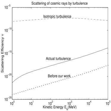
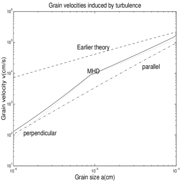
Figure 4.: Applications. (By Lazarian & Yan). Left: Cosmic ray scattering for the actual MHD turbulence is reduced substantially compared to scattering by isotropic turbulence but larger than estimates in Chandran (2000). Right: The dust acceleration by turbulence is reduced compared to the accepted estimates in Draine (1985).

5.2. Grain dynamics

Turbulence induces dust grain relative motions and causes grain-grain collisions. Those determine grain size distribution which affects most of the dust properties including absorption and H₂ formation. Unfortunately, as in the case of cosmic rays, the earlier research appealed to hydrodynamic turbulence to predict grain relative velocities (see Kusaka et al. 1970; Volk et al. 1980; Draine 1985; Ossenkopf 1993; Weidenschilling & Ruzmaikina 1994).

The differences between the hydrodynamic and MHD calculations stem from (a) grain being charged and thus coupled with magnetic field, (b) anisotropy of MHD cascade, and (c) direct interaction of charged grains with magnetic perturbations. Effects (a) and (b) are considered in Lazarian & Yan (2002), while (c) is considered in Yan & Lazarian (2002b; in preparation). As the consequence of these studies the picture of the grain dynamics is substantially altered.

Consider grain charge first. If grain’s Larmor time $\tau_{L}=2\pi m_{gr}c/qB$ is shorter than gas drag time $t_{drag}$, grain perpendicular motions are constrained by magnetic field. Their velocity dispersion are determined by the turbulence eddy whose turnover period is $\sim\tau_{L}$ instead of drag time (Draine 1985).

Accounting for the anisotropy of MHD turbulence it is convenient to consider separately grain motions parallel and perpendicular to magnetic field. The perpendicular motion is influenced by the Alfven mode, which has a Kolmogorov spectrum. The parallel motion is subjected to compressible modes with scaling $v_{\parallel}\propto k_{\parallel}^{-1/2}$. In addition we should account for turbulence damping via viscous forces. When the eddy turnover time is of the order of $t_{damp}\sim\nu_{n}^{-1}k_{\perp}^{-2}$, the turbulence is viscously damped. Thus grains sample only a part of the eddy before gaining the velocity of ambient gas if $\tau_{L}$ or $t_{drag}<t_{damp}$. The results are shown in Fig. 4b.

The direct interaction of the charged grains with turbulent magnetic field results in a stochastic acceleration that can potentially provide grains with supersonic velocities.

6. Summary

Recently there have been significant advances in the field of MHD turbulence:

1. The first self-consistent model (GS95) of incompressible MHD turbulence that is supported by both numerical simulations and observations has been suggested. The major predictions of the model are scale-dependent anisotropy ($k_{\|}\propto k_{\perp}^{2/3}$) and a Kolmogorov energy spectrum ($E(k)\propto k^{-5/3}$).

2. Simulations of compressible MHD turbulence show that there is a weak coupling between Alfven waves and compressible MHD waves and that the Alfven modes follow the Goldreich-Sridhar scaling. Fast modes, however, decouple and exhibit isotropy.

3. On the contrary to the general belief, in typical interstellar conditions, magnetic fields can have rich structures below the scale at which motions are damped by viscosity created by neutrals (ambipolar diffusion damping scale).

These advances change a lot in our understanding of many fundamental interstellar processes, e.g. cosmic-ray propagation and grain dynamics. In terms of HI they show a way to account for the formation of structures at very small scales. More discoveries are surely to come!

Acknowledgments.

We thank Ethan T. Vishniac and Peter Goldreich for valuable discussions. We acknowledge the support of NSF Grant AST-0125544. This work was partially supported by National Computational Science Alliance under CTS980010N and AST000010N and utilized the NCSA SGI/CRAY Origin2000.

References

Andrews, S. M., Meyer, D. M., & Lauroesch, J. T. 2001, ApJ, 552, L73

Armstrong, J. W., Rickett, B. J., & Spangler, S. R. 1995, ApJ, 443, 209

Cesarsky, C. 1980, Annu. Rev. Astro. Astrophys., 18, 289

Chandran, B. 2001, Phys. Rev. Lett., 85(22), 4656

Cho, J. & Vishniac, E. T. 2000, ApJ, 539, 273

Cho, J., Lazarian, A., & Vishniac, E. T. 2002a, ApJ, 564, 291 (CLV02a)

Cho, J., Lazarian, A., & Vishniac, E. T. 2002b, ApJL, submitted (astro-ph/0112195)

Deshpande, A.A., Dwarakanath, K.S., & Goss, W.M. 2000, ApJ, 543, 227

Dieter, N.H., Welch, W.J., & Romney, J.D. 1976, ApJ, 206, L113

Draine, B.T. 1985, in Protostars and Planets II, ed. D. C. Black & M. S. Matthews (Tucson: Univ. Arizona Press)

Goldreich, P. & Sridhar, H. 1995, ApJ, 438, 763 (GS95)

Heiles, C. 1997, ApJ, 481, 193

Higdon, J.C. 1984, ApJ, 285, 109

Iroshnikov, P. 1963, Astron. Zh., 40, 742 (English: 1964, Sov. Astron., 7, 566)

Kolmogorov, A. 1941, Dokl. Akad. Nauk SSSR, 31, 538

Kota, J. & Jokipii, J. R. 2000, ApJ, 531, 1067

Kraichnan, R. 1965, Phys. Fluids, 8, 1385

Kulsrud, R.M. & Anderson, S.W. 1992, ApJ, 396, 606

Kusaka, T., Nakano, T., & Hayashi, C. 1970, Prog. Theor. Phys., 44, 1580

Larson, R. B. 1981, MNRAS, 194, 809

Lazarian, A. & Pogosyan, D. 2000, ApJ, 537, 720

Lazarian, A.& Vishniac, E. T. 1999, ApJ, 517, 700

Lazarian, A., Vishniac, E. T., & Cho, J. 2002, in preparation

Lazarian, A. & Yan, H. 2002, ApJ, submitted

Leamon, R. J., Smith, C. W., Ness, N. F., & Matthaeus, W. H. 1998, J. Geophys. Res., 103, 4775

Mac Low, M. 1999, ApJ, 524, 169

Maron, J. & Cowley, S. 2002, astro-ph/0111008

Maron, J. & Goldreich, P. 2001, ApJ, 554, 1175

McKee, C. F. 1999, in The Origin of Stars and Planetary Systems, ed. J. L. Charles & D.K. Nikolaos (Dordrecht: Kluwer), 29

Minter, A. & Spangler, S. 1997, ApJ, 485, 182

Monin, A.S. & Yaglom, A.A. 1975, Statistical Fluid Mechanics: Mechanics of Turbulence, Vol. 2 (Cambridge: MIT Press)

Myers, P.C. 1983, ApJ, 270, 105

Myers, P.C. 1999, in The Origin of Stars and Planetary Systems, ed. by J.L. Charles & D.K. Nikolaos (Dordrecht: Kluwer), 67

Müller, W.-C. & Biskamp, D. 2000, Phys. Rev. Lett., 84(3) 475

Ossenkopf, V. 1993, A&A 280, 617

Scalo, J. M. 1984, ApJ, 277, 556

Scalo, J. M. 1987, in Interstellar Processes, ed. D. J. Hollenbach & H. A. Thronson (Dordrecht: Reidel), 349

Schlickeiser, R. & Miller, J.A. 1998, ApJ, 492, 352

Stanimirovic, S. & Lazarian, A. 2001, ApJ, 551, L53

Vishniac, E. T. & Cho, J. 2001, ApJ, 550, 752

Volk, H. J., Jones, F. C., Morfill, G. E., & Roser, S. 1980 A&A, 85, 316

Weidenschilling, S. J. & Ruzmaikina, T. V. 1994, ApJ, 430, 713