The field of NGC 6397 as a test for Galactic models

Abstract

Taking advantage of recent HST data for field stars in the region of the Galactic globular cluster NGC 6397, we tested the predictions of several Galactic models with star counts reaching a largely unexplored range of magnitudes, down to $V$$\sim$ 26.5. After updating the input stellar ($V-I$) colors, we found that the two-component Bahcall-Soneira (B&S) model can be put in satisfactory agreement with observations for suitable choices of disk/spheroid luminosity functions. However if one assumes the Gould, Bahcall and Flynn (1996, 1997) disk luminosity function (LF) together with the Gould, Flynn and Bahcall (1998) spheroid LF, there is no way to reconcile the predicted and observed $V\,$-magnitude distribution. We also analysed the agreement between observed and predicted magnitude and color distributions for two selected models with a thick disk component. Even in this case there are suitable combinations of model parameters and faint magnitude LFs which can give a reasonable agreement with observational star counts both in magnitude and in color, the above quoted combination of Gould et al. (1997, 1998) LFs giving again predictions in clear disagreement with observations.

1 Introduction

Since the very beginning of modern astronomy, the distribution of stars over the night sky has been understood as evidence for the spatial distribution we now know as “the Galaxy”. Therefore, the use of star counts to constrain the Galactic structure has been the goal of generations of astronomers. In the long run, relevant progresses on that matter has been allowed by the increased amount of observational data, by the availability of modern computers and, last but not least, by the original approach to the problem presented twenty years ago in a seminal paper by Bahcall & Soneira (1980, see also 1984). Since that time star counts began an effective way of investigating the broad properties of stellar populations in our Galaxy (see e.g. Gilmore 1981, 1984, Gilmore & Reid 1983 and for a review Bahcall 1986 and Gilmore, Wyse & Kuijken 1989).

Galactic models, which predicts star counts in selected areas of the sky and for selected intervals of magnitude, give, at the same time, constraints about such relevant issues as the amount of mass in the form of stars and, in particular, about the contribution of faint stars to the dark-matter problem. One naturally expects that the contribution of intrinsically faint stars increases as the limiting magnitude of star counts is increased. Thus the limiting magnitude of the observational samples is a critic factor governing the possibility of constraining the Galactic abundance of such kind of stars. However, the difficulty in distinguishing faint images of stars from galaxies has limited most of the ground based work to V $\,\stackrel{{\scriptstyle<}}{{{}_{\sim}}}\,$ 20, reaching as extreme limit V$\approx$ 22 (e.g. Bahcall 1986, Reid & Majewski 1993, Haywood et al. 1997 and references therein).

This situation has been recently improved by observational data from the Hubble Space Telescope (HST). HST observations reach very faint magnitudes (V$\approx$30, see e.g. Williams et al. 1996) and even though the number of stars in the field of view is generally quite small they can be used to test Galactic models at the best resolution available. However the tests of Galactic models at faint magnitudes available in the literature are still very few and mainly based on a restricted number of stars (see Mendez et al. 1996, Reid et al. 1996, Basilio et al. 1996, Mendez & Guzman 1998).

In this paper we will take advantage of recent HST observations of the Galactic globular cluster NGC 6397, to discuss a rich sample of about thousand bona fide Galactic field stars which should be fairly complete (more than 95% detection level) down to $V\sim$ 25, with a reliable evaluation of the completeness reaching $V\sim$ 27 (King et al. 1998, hereafter KACP). This sample obviously gives the exciting opportunity of testing Galactic models over an almost unexplored range of magnitudes, with possible relevant outcomes concerning the abundance of faint stars. For the analysis we will use observational data of field stars in the direction of NGC 6397 from the second epoch HST observations. Field stars have been obtained by an accurate separation from cluster stars based on proper motions analysis (KACP). The area covered by observations is of 6.6 arcmin² centered at the Galactic coordinates $l=337^{\circ}.9$, $b=-11^{\circ}.7$. Figure 1 shows the $(V-I,V)$ color–magnitude diagram for the about 1000 stars whose proper motion is significantly different from that of the NGC 6397 stellar population (cf. Fig.1 in KACP).

In Section 2 we will use these data to discuss the predictions of the Bahcall-Soneira Galaxy model (Bahcall 1986) which has been widely used by observers to predict the number of stars of different types, colors and apparent magnitude ranges in different fields of interest (see e.g. Boeshaar & Tyson 1985, Flynn & Freeman 1993, Lasker et al. 1990, Stuwe 1990, Basilio et al. 1996). Bahcall and Soneira assumed that the Galaxy is simply composed by a disk, with a scale height of a few hundred parsecs, and a more or less spherical spheroid. The Bahcall-Soneira model, as further improved mainly to account for interstellar reddening and obscuration, was proved to be in good agreement with available observations (see e.g Bahcall 1986, Gould, Bahcall & Maoz 1993 and references therein) and the export code was made available on the Web to the scientific community in 1995. However at faint magnitudes such an agreement is strongly dependent on the assumption about the luminosity function (LF) of faint main sequence (MS) stars. As a result, in Sect.3, we will show that the above quoted agreement vanishes for several recent evaluations of the actual LF of either the disk or the halo components.

The need for more complex Galactic models has been advanced in 1983 by Gilmore & Reid, who firstly suggested the occurrence of an extended “thick disk” population consisting of stars with spatial and kinematic properties intermediate between disk and spheroid. Starcounts is not the best way to constrain this third component because similar results could be obtained either with a thick disk or without it in dependence of the adopted model parameters (disk/thick disk scale height, scale lenght and normalizations). However detailed analysis which, in addition to the star counts, take into account the velocity distribution of local stars, support the need for a thick disk component (Ojha et al. 1996, Wyse & Gilmore 1995, Norris & Ryan 1991, Casertano, Ratnatunga & Bahcall 1990.)

However up to now, sensitively different values for the thick disk structural parameters (density law, local density etc..) have been proposed (see e.g. Reid & Majewski 1993, Yamagata & Yoshii 1992, Ojha et al. 1996, Mendez & Guzman 1998). Thus the situation is not yet well defined and in Sect.4 we will use our data to test some three-component models currently available in the literature. In this context, one has to remind that with very faint observations it should be possible to resolve the Galaxy into its component populations. This because for V$>$19, at least for high Galactic latitudes, the various components are expected to contribute with different colors: the bluer colors are dominated by spheroid stars, the reddest objects do belong to the disk population, while the intermediate colors should be dominated by thick disk stars (see Basilio et al. 1996).

Unfortunately, our data refer to a sky region of somewhat low latitude, which gives a sensitive gain in the number of stars but which - as we will find - makes difficult a clear separation among the various populations. As a result we will find that either two-component or three component models give an equally satisfactory agreement with magnitude and color observational counts. No one of the current Galactic models appears in agreement with observations for some extreme assumptions on the faint LF, whereas the data do not allow to discriminate between different three-component models within the current uncertainties on the scale height and on the density of stars in the solar neighbourhood.

Figure 1: The $(V,V-I)$ CM diagram for the sample of field stars studied.

2 The B&S model

As first step we compared color and magnitude distributions from our observational sample to the predictions of the Bahcall-Soneira model in its original export version (see Bahcall, 1986, for a complete description of the model). For convenience in the following we will briefly summarize the main parameters (see also table 1:
i) Disk. The disk has a Wielen (1974) luminosity function and an exponential scale lenght of 3.5 kpc. The scale height for the later main sequence (M_V$>$5) is 325 pc. For the early main sequence (M_V$<$5) it is (82.5 M_V $-$ 97.5) pc with a minimum of 90 pc. The scale height of the giant branch is 250 pc.
ii) Spheroid. The spheroid has the same LF as the disk implemented for M_V$\leq$4.5 with the 47 Tuc luminosity function (Da Costa, 1982), shifted to fit the Wielen LF at M_V$\approx$4.5. The Galactocentric distance is R_∘=8 kpc and the axis ratio is 0.8. The density is normalized locally at 1/500 of the disk.

For each stellar population it is possible to associate intrinsic stellar magnitudes with colours, predicting in such a way the expected colour distribution of stars in each given interval of magnitudes. The original version of the B&S model adopts as relations between (B-V) colors and absolute visual magnitudes, a disk main sequence (MS) from observations by Johnson (1965,1966) and Keenan (1963) and the color-magnitude (CM) diagram of M67 by Morgan & Eggleton (1978) for disk giant stars. The program allows the choice of the spheroid giant branch from a number of different color-magnitude diagrams (e.g. 47 Tuc, M13, M15, M92) while the main sequence adopted for the disk is shifted to properly match the evolved stars of the selected diagram, reproducing in this way the different colors of the spheroid MS as a function of the assumed metallicity.

Figure 2 compares the distribution of apparent $V\,$-magnitudes of the sample stars with the corresponding predictions produced by a straightforward application of the B&S model. The observed magnitude distribution plotted in Fig.2 has been corrected for incompleteness as in KACP (cf. Tab. 1 in KACP), restricting the investigation to the range of magnitudes with completeness larger or of the order of 80%. i.e. to stars with $V\leq 26.5$ . As shown in Fig.2, one finds a good agreement over the whole accepted range of magnitudes, with theoretical predictions almost always within the expected statistical fluctuation of the counts. As expected, at these low latitudes, counts are dominated by disk stars. Thus, as we will discuss better later, the total distributions are barely sensitive to the presence of a possible third component.

Figure 2: The histogram of the observed magnitudes as compared with theoretical predictions by the B&S model. Observations are corrected for incompleteness. Error bars give the expected 1$\sigma$ statistical fluctuations of the observed counts in the completeness region. Heavy dashed and dot-dashed lines represent the contribution to the total counts of the disk or the spherical component, respectively. Thin dot-dashed and dotted lines show the results for the spheroid and the corresponding total counts when the cut-off for the spheroid luminosity function is introduced (see text).

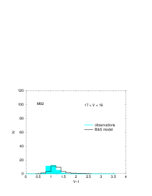
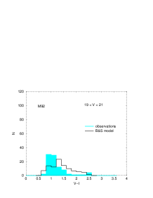
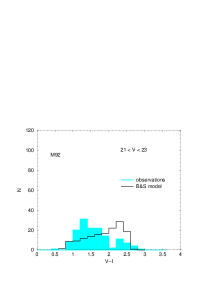
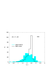
Figure 3: Comparison between the observed (shaded region) and predicted distribution of ($V-I$) colours in the labelled intervals of magnitude. The adopted ($M_{V}$,$V-I$) relations for MS stars are as in Fig.4, upper panel, while the ($M_{V}$,$V-I$) relations for RGB stars are derived from the CMDs of M67 (Morgan & Eggleton 1978) and M92 (Sandage 1970) for disk and spheroid stars respectively. The adopted color dispersion is $\sigma$=0.06 (see e.g. Bahcall & Soneira, 1980).

The observational data can also be used to test predicted color distributions. We used the M_V-(B-V) relations described above together with the relations from ($B-V$) to ($V-I$) colour bands for MS and giant stars obtained from Johnson (1965, 1966) observational data, as suggested in the original B&S code. Figure 3 shows that, in this case, the agreement is far from being satisfactory, the difference between predictions and observations becoming worse at fainter magnitude. Thus while V magnitudes are well reproduced, $(V-I)$ colour distributions are not. The origin of such an occurrence is easily understood, since inspection of the B&S data discloses that the adopted ($M_{V}$, $B-V$) diagram for the two stellar populations was still in excellent agreement with recent results from the Hipparcos satellite for nearby stars (Kovalevsky 1998), whereas this is not the case for the ($M_{V}$, $V-I$) distributions. To be quantitative, the upper panel in Fig. 4 compares the adopted B&S ($M_{V}$,$V-I$) distributions for disk and spheroid MS stars with recent data by Monet et al. (1992) and Dahn et al. (1995) for dwarf and subdwarf stars in the solar neighbourhood; the need to update the M_V-($V-I$) relations appears obvious. In passing we note that the B&S model was never compared by the authors with ($V-I$) color distributions thus they had not the need to introduce in the code precise relations for this color band. We derived a new ($M_{V}$, $V-I$) relation for the disk population by best fitting the above-cited observational data for dwarf stars.

Figure 4: Upper panel: The (M_V, V-I) relations adopted in the original B&S model as compared with the CM diagram of stars in the solar neighbourhood. Lower panel: the same as in the upper panel but for the “new” (M_V, V-I) relations (see text).

In order to keep our computations as close as possible to the original B&S model, we choose for the spheroid a $Z=0.0002$ MS as defined by HST in the very metal-poor globular M30 (Piotto et al. 1997). The bottom panel of Fig.4 shows the new sequences as compared with the same observational data in the upper panel. Here we notice that the excellent agreement recently found between theoretical predictions and HST observations of faint MS in Galactic globulars (Cassisi et al. 2000) supports the use of theoretical data in varying the adopted spheroid metallicity. Thus in the lower panel of Fig.4 the low MS at Z=0.002 is from evolutionary calculations by Cassisi et al. (2000). Finally, ($M_{V}$,$V-I$) relations for giants stars that have left the MS have been taken from the CM diagrams of M67 (Montgomery, Marshall & Janes 1993) and M92 (Johnson & Bolte 1998) for disk and spheroid stars, respectively.

However, even if relying on observational data, one can not ignore that all the available theories unanimously predict that the location of the lower mass limit for H burning is strongly dependent on the star’s metallicity and, in particular, that for $Z=0.0002$ this limiting magnitude is $M_{V}=14.2$ (see, e.g., again Cassisi et al. 2000). To be realistic, we thus used this magnitude as a cut-off of the luminosity function of the spheroid component. Numerical experiments, as reported in the previous Fig.2, shows that such a cut-off is predicted to affect the distribution of the observed luminosities only at magnitudes fainter than $V=28$, thus beyond the limit of the present investigation. However, it appears interesting to notice that, at least in principle, observational data below $V\sim$28 should constrain the magnitude of the cut-off, and, therefore, the mean metallicity of the spheroid component.

Before comparing theory and observation with the new color-magnitude relations, it is useful to discuss the adopted reddening correction. The original version of the code incorporates for intermediate-to-high Galactic latitudes ($\mid b\mid\geq$10^∘) the “default” reddening/obscuration correction through “infinity” from Sandage (1972) based on Galaxy counts, which gives in the direction of NGC 6397 a reddening E(B-V)$\approx$0.26. However we prefer to adopt the more precise and extensively used reddening maps by Burnstein & Heiles (1982). For their reddening estimates the authors used together the results of surveys of neutral hydrogen column densities and of deep Galactic counts. The Burnstein & Heiles compilation gives E(B-V)$\approx$0.18 in the direction of NGC 6397, a value in good agreement with reddening estimates for the cluster from different methods: E(B-V)=0.18 $\pm$0.02 (see e.g. Harris 1996, Anthony-Twarog et al. 1992, Drukier et al. 1993). Thus, in the following, we will adopt E(B-V)=0.18 transformed in E(V-I) by using E(V-I)$\approx$1.25 E(B-V) by Bessel & Brett (1988). The reddening scale height adopted in the program is 100 pc (see e.g. Mendez & van Altena, 1998).

The difference between Sandage (1972) results and these estimates for the reddening/obscuration correction clearly affects both magnitude and colors distributions in a small but not negligible way; the magnitude distribution is shifted by about 0.2 mag. toward brighter magnitudes due to the reduced extinction, while the color distribution in the interval 23$<$V$<$25 is shifted toward bluer colors by about 0.2 mag. and the total counts in this interval are increased due to the change in the extinction. In passing we note that the NGC 6397 field is just above the lower limit ($\mid b\mid=10^{\circ}$) of Galactic latitudes covered by the reddening treatment by Burnstein & Heiles (1982).

Figure 5 shows the effect of improving both the reddening and ($M_{V}$, $V-I$) relations for the predicted colour distributions in the same magnitude interval as in Fig.3. The agreement now appears rather satisfactory, showing that with such a minor modifications the B&S model appears able to fit all the observational constraints reasonably well. Numerical simulations show that results do not change significantly if we assumed Z=0.002 as spheroid mean metallicity.

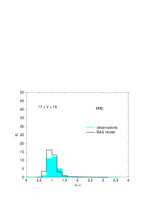
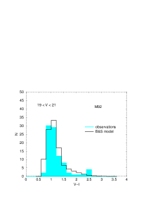
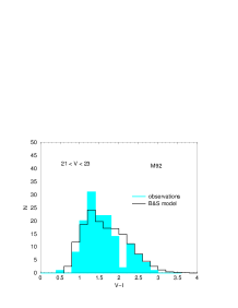
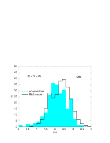
Figure 5: Comparison between the observed and predicted $V-I$ color distributions for the labelled intervals of magnitude. The adopted ($M_{V}$,$V-I$) relations for MS stars are as in Fig.4, lower panel, while for the ($M_{V}$,$V-I$) relation for spheroid RGB stars we adopted the M92 color-magnitude diagram from Johnson & Bolte (1998). The adopted reddening is E(V-I)=1.25 E(B-V), with E(B-V)=0.18, see text.

3 The faint star problem

The excellent agreement between theory and observation discussed in the previous section is not without problems. At present time one has much more information about the faint end of the disk luminosity function than at the time when the original B&S model was produced. As a matter of fact, below $M_{V}$=12.5 the original version of the B&S model assumes a flat luminosity function both for the disk and the spheroid component. However, several lines of evidence have been found indicating that in both populations the luminosity functions undergo a noticeable decrease at the faintest luminosities. Figure 6 (upper panel) shows recent observational data for the faint end of the disk luminosity function together with the distribution originally assumed in the B&S model.

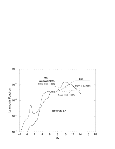
Figure 6: Upper Panel: Disk luminosity functions as determined by Wielen et al. (1983) heavy solid line, Gould et al. 1997 (heavy short dashed line), Reid & Gizis 1997 (dot-dashed line) and Martini & Osmer 1998 (long dashed line). The original B&S choice for the disk LF (Wielen 1974 and a constant value for M_V$<$12.5) is also shown (thin solid line). Lower Panel: Spheroid luminosity functions as determined by Gould et al. 1998 (dashed line) and Dahn et al. 1995 (dot-dashed line) together with M30 LF from Sandquist (1999) and Piotto et al. (1997), observational data (heavy solid line). The original B&S choice for the spheroid LF (the same as the disk LF for M_V$\geq$4.5 implemented with the 47 Tuc luminosity function as measured by Da Costa (1982) for M_V$\leq$4.5) is also shown (solid line).

A decrease of the luminosity function beyond $M_{V}$= 13 has been firstly suggested by Wielen, Jahreiss and Kruger (1983, WJK), on the basis of parallax-star studies. An even more drastic decrease, starting at $M_{V}$= 12, was more recently suggested by Gould, Bahcall and Flynn (1996, 1997) from an analysis of HST data. The results from a large-area multicolor survey by Martini and Osmer (1998) and those from photometric parallax surveys by Reid & Gizis (1997) appear intermediate between the Wielen et al. and the Gould et al. results. All these luminosity functions fit the Wielen et al. LF at a visual magnitude of about 9.

Figure 6, lower panel, shows the situation for the spheroid component. Again there is not agreement among the results of different authors. Dahn et al. (1995) from parallaxes studies of nearby subdwarf stars found a peak of the luminosity function at $M_{V}$ $\approx$ 11.5. However, Gould, Flynn and Bahcall (1998) investigated HST data and suggested a flat LF below $M_{V}$= 7, while very recently Gizis & Reid (1999), by using a sample of stars from the Palomar Sky Surveys, support the luminosity function results by Dahn et al. (1995). The original B&S choice for the spheroid LF is also shown.

An extensive investigation of the luminosity functions in Galactic globulars has recently shown the common occurrence of a maximum near $M_{V}\sim$10 (Piotto, Cool & King 1997, Piotto & Zoccali 1999). In the same panel of Fig. 6 we show the luminosity function of the metal-poor Galactic globular M30, as obtained down to $M_{V}$$\sim$8 by Sandquist et al. (1999) and extended below $M_{V}$$\sim$8 with the LF of M30 provided by Piotto et al. (1997). M30 is a metal poor cluster that we will assume as possibly representative of the spheroid luminosity function. The rationale for this choice follows from the assumption of a substantial similarity between field and cluster spheroid populations. In this context, one may take note of the different LFs observed in Galactic globulars (see, e.g., Piotto & Zoccali 1999) as an evidence for a different efficiency of the evaporation of low-mass stars from the clusters, a mechanism which is obviously impoverishing the faint end of the original LFs. By adopting M30 we choose one of the globulars with the largest abundance of faint stars, thus with a LF which should be closer to the original one for spheroid stellar content.

Dahn et al.(1995) and Gould et al. (1998) LFs rejoin each other at M_V$\approx$ 7.5 mag. to match the B&S LF. M30 LF has been normalized to fit at M_V$\approx$7 the spheroid LFs (see Gould et al. 1998). In passing we note that the difference between the M30 luminosity function and the original choice of B&S for M_V$<$6 is mainly due to the normalization chosen by the authors: the luminosity function of 47 Tuc (for M_V$<$4.5) has been shifted to connect to the Wielen LF at M_V=4.5. However numerical experiments show that, due to the poor population of the high luminosity LF regions, the quoted differences for M_V$<$6 affects only slightly magnitude and color distributions, while difference in the LF for M_V$<$4.5 does not influence at all the results. In the following we will choose to adopt the M30 LF at brigh magnitudes (M_V$<$6).

We are now in the position to explore the role played on the predicted star counts by the faint portion of the luminosity function. Fig.7 shows the predicted magnitude distribution of disk and spheroid stars when different LFs have been adopted. For comparison the histogram of the observed counts in the field of NGC 6397 is also shown. These results are easily understood on the basis of the shape of the adopted LFs.

Figure 7: Upper Panel: Theoretical magnitude distribution for disk stars when different disk LFs of Fig.6 (upper panel) are used. Lower Panel: Theoretical magnitude distribution for spheroid stars when the spheroid LFs of Fig.6 (lower panel) are used. The adopted reddening is E(B-V)=0.18. The spheroid/disk local normalization is 1/500.

From the results of Fig.7 one also easily understand the magnitude distribution for the different combinations of disk and spheroid LFs shown in Fig.8. As a first result, one finds that different assumptions about the faint end of the luminosity function affect star counts only for V $\,\stackrel{{\scriptstyle>}}{{{}_{\sim}}}\,$ 23 (see Fig.7 and Fig.6). If one takes the already known capability of the B&S model to pass the observational tests down to $V$$\sim$ 21 as an evidence that the model gives a satisfactory description of the Galactic distribution of the most luminous components of the stellar populations, one would conclude that the abundance of fainter stars depends only on the overall behaviour of the LFs.

By assuming the Gould et al. (1996, 1997) disk LF together with the Gould et al. (1998) spheroid LF (thin solid line in Fig. 8) there is no way to reconcile the predicted and observed $V$-magnitude distributions. Since star counts are governed mainly by the disk component, by assuming the Gould et al. (1997) disk LF one predicts a number of faint stars smaller than observations in the last two magnitude bins, even assuming for the spheroid component the M30 LF, which gives the largest counts at faint magnitudes (long dashed line in Fig.8). Similarly by adopting the Gould et al. (1998) spheroid LF the model underestimates the observed counts in the last two bins of magnitude for any choice of the disk LF (dot-dashed line and thin solid line in Fig.8).

However the reliability of star counts in the last magnitude bin: 26$<$M_V$<$26.5 is important to evaluate if the Gould et al. (1997) LF for the disk or the Gould et al. (1998) LF for the halo are separately acceptable for our field. We note that in the last bin (from M_V=26 to M_V=26.5) the completeness falls from about 90% to about 80%. If, very conservatively, we decide do not take into account the results in this bin of magnitude we cannot exclude the separate adoption either of the Gould et al. (1997) LF for the disk or of the Gould et al. (1998) LF for the halo, excluding however the contemporary adoption of both LFs.

Figure 8: As in Fig.2 but for the theoretical magnitude distributions obtained for the two-component B&S model with the labelled combinations of disk/spheroid LFs.

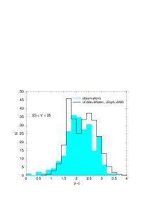
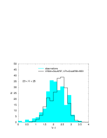
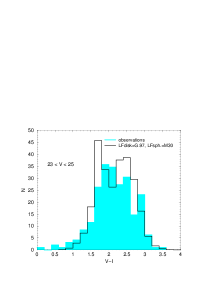
Figure 9: Theoretically predicted colour distributions for 23$<$V$<$25 for the models of Fig.8, as compared with observational data (shaded region). Upper left panel: Wielen et al. (1983) disk LF + Dahn (completed with M30) spheroid LF. Upper Righ Panel: Wielen et al. disk LF + M30 LF for the spheroid. Lower Left Panel: Gould et al. (1997) for the disk LF and Gould et al. (1998) for the spheroid LF. Lower Right Panel: Gould et al. (1997) for the disk LF and M30 for the spheroid LF.

Figure 8 shows that it is possible to find several combinations of LFs for disk/spheroid which fit the observational magnitude distribution in a better way. However, due to the large uncertainties still present in the determination of disk and spheroid LFs this seems to us a meaningless numerical exercise. Figure 9 shows the predicted color distribution in the region 23$<$V$<$25 (the only affected by the changes in the adopted LFs) for the combinations of LFs shown in Fig.8. All the results are in fair agreement with observational color distributions. Thus Fig.9 does not allows to discriminate among different LFs.

4 Models with thick disk

In the previous sections we have shown that the two-component (disk + spheroid) B&S model, appears able to reach a satisfactory agreement with the deep star counts provided by HST in the field of NGC 6397 only if LFs are larger than expected on the basis of Gould et al. (1997,1998) indications. In this section we will include a thick disk component to check if such a conclusion is affected by the addition of a third component to the Galactic structure.

In 1993 Gould et al. discussed photometric data from the Hubble Space Telescope Snapshot Survey up to an average apparent magnitude of V=21.4 to conclude that, mainly due to the lack of information about the colors of the observed stars, it was not possible to distinguish between the presence or the absence of the thick disk. In 1996 Basilio et al. used I magnitude and ($V-I$) color star counts from 17 HST deep fields data to discriminate between the results of the standard models by Bahcall & Soneira (1980,1984) and by Gilmore & Reid (1983). They concluded that the two standard model predictions for the magnitude counts was similar and in good agreement with observations. However they obtained a reasonable agreement between model and data for colour distributions only with the introduction of a thick disk component. Mendez & Guzman (1998) by adopting a small data sample with V up to $\approx$25 found an equally good agreement between models with thick disk and observations for a thick disk with a local normalization of 2% and a scale height of 1300 pc (Reid & Majewski 1993) or a local normalization of 6% and a scale height of 750 pc (Ojha et al. 1996). More in general, one finds that a large variety of disk/thick disk parametrizations is available in literature (see e.g. Reid & Majewski 1993, Ojha et al. 1996).

For our first test we adopted a consistent set of disk/thick disk/spheroid parameters as given for the “Besancon model” by Haywood, Robin & Creze (HR&C, 1997, see also Haywood, Robin & Creze 1996, Ojha et al. 1996, Robin et al. 1996 for more details). The disk /thick disk luminosity function adopted by the authors is from Wielen et al. (1983) for M_V$>$4, from McCuskey (1966) for M_V $<$-1 and an average of both LFs in the interval -1$\leq$ M_V $<$4. The chosen parameters are: a disk scale height of 240$\pm$50 pc, a thick disk scale height of 760$\pm$50 pc, a disk scale lenght of 2500$\pm$300 pc, a thick disk scale lenght of 2500$\pm$800 pc, a thick disk/disk local density ratio of 5.6$\pm$1%, a spheroid/disk local density ratio of 0.10%, R_∘=8.5 Kpc (see HR&C). However the “Besancon” model explicity allows for time evolution of vertical scaleheight whereas the other models implicit take into account this variation by assigning lower scaleheights to early-type dwarfs. Thus here we will take a scale height of 90 pc for the youngest MS stars and 240 pc for the oldest ones.

To explore the range of possible results, we made tests by adopting either Wielen et al. (1983) or Gould et al. (1997) disk and thick disk LFs for selected assumptions about the spheroid LF and by adopting for the thick disk LF at bright magnitudes (M_V$<$4.5) the LF of 47 Tuc (Hesser, Harris & Vandenberg, 1987), assumed more representative of high luminosity thick disk stars. However numerical results show that by replacing, for M_V$<$4.5, the 47 Tuc LF with the Wielen et al. LF the differences in the resulting star counts, at least for our field, are small.

Figure 10 shows the theoretical magnitude distributions when different disk/thick disk and spheroid luminosity functions are used. The contribution of the thick disk component is also shown. The dashed line represents a model with Wielen et al. (1983) disk/thick disk luminosity function and Gould et al. (1998) spheroid LF at faint magnitudes (M_V$>$ 8) implemented at brighter magnitudes by M30 LF (Sandquist 1999). The solid line represents a model with Gould et al. (1997) disk/thick disk LF and with Dahn et al. (1995) spheroid LF at low luminosities completed with M30 for (M_V$<$ 8). As expected, one finds again that the distribution is affected by the change of the faint LF only for M_V $\,\stackrel{{\scriptstyle>}}{{{}_{\sim}}}\,$ 24. However now one finds that the three-component model with the parameters described above slightly overestimates the counts up to (M_V$\approx$24). Comparison with results in Fig.8 shows that predictions based on Gould et al. (1998) LF appear in better agreement with faint star counts (see e.g. the case of Wielen et al. disk LF and Gould et al., 1998, spheroid LF).

Figure 10: The histogram of the observed magnitudes (as in Fig. 2) as compared with theoretical predictions by the B&S model with a thick disk component with parameters as in Haywood et al. (1997) (HR&C). The results for the two labelled different combinations of disk (thick disk)/spheroid LFs are shown (see text). The contribution of the thick disk component to the total counts is also shown.

Figure 11: Upper panel: comparison between observational data and predicted magnitude distributions for a three-component model with Gilmore & Reid (G&R, 1983) parameters and Haywood et al. (HR&C, 1997) parameters (see text). The adopted LFs are Wielen et al. (1983) for the disk/thick disk (completed in this last case with the LF of 47 Tuc) and Gould et al. (1998), completed with M30 for M_V$<$ 8, for the spheroid. The contribution to the total counts of the two thick disk components are also shown. For comparison the two components B&S model with the same disk/spheroid LFs is also shown. Lower panel: contribution to the star counts of the disk/spheroid components for the three selected models.

Table 1: Parameters of the two components Bahcall-Soneira (B&S) model and of the models with thick disk by Haywood, Robin & Creze (HR&C) and by Gilmore & Reid (G&R), see text for more details.

Models		B&S	G&R	HR&C
Disk	scale height (pc)	325	325	240$\pm$50
	scale lenght (pc)	3500	3500	2500$\pm$300
Thick Disk	scale height (pc)	—-	1300	760$\pm$50
	scale lenght (pc)	—-	3500	2500$\pm$300
	thick disk/disk	—-	2%	5.6$\pm$1%
	density ratio
Spheroid	spheroid/disk	0.200%	0.125%	0.100%
	density ratio
	axis ratio	0.8	0.8	0.8

Before discussing such an evidence, as an alternative choice, let us now explore the model by Gilmore & Reid (1983) by adopting their most frequently used parameters (G&R, 1983, 1984, see also Colless et al. 1991, Basilio et al. 1996). The chosen parameters are: an disk scale height of 325 pc, a thick disk scale height of 1300 pc, a thick disk scale lenght of 3500 pc, a thick disk/disk local density ratio of 2%, a spheroid/disk local density ratio of 0.125% with, as in Reid & Majewski (1993), similar LFs for both disk and thick disk. Reid & Majewski (1993) adopted for disk/thick disk luminosity function the Wielen et al. (1983) LF for M_V$<$ 11 implemented at fainter magnitudes with the photometric-parallax-based LF by Reid (1987) which is not too much different from the Reid & Gizis one, shown in Fig.6 and thus it is intermediate among the Wielen et al. (1983) and Gould et al. (1997) one. For reader’s convenience, table 1 summarizes the main disk/thick disk/spheroid parameters of the selected galactic models.

Figure 12: The histogram of the observed magnitudes (as in Fig. 2) as compared with theoretical predictions by the B&S model with a thick disk component with parameters as in Haywood et al. (1997) (HR&C) for the labelled combinations of disk/thick disk/spheroid LFs at faint magnitudes. The thick disk parameters are: scale height = 710 pc and thick disk/disk local density ratio of 4.6% (see text). The contribution of the thick disk component to the total counts is also shown.

Fig.11 (upper panel) shows the comparison between the predicted magnitude distribution for a model with the parameters of the “Besancon model” and the one with the Gilmore & Reid model parameters. The adopted luminosity functions are Wielen et al. (1983) for disk and thick disk and Gould et al. (1998) + M30 for the spheroid. One sees that the predictions of the two models are coincident in the whole region of interest (M_V $\mbox{$\,\stackrel{{\scriptstyle<}}{{{}_{\sim}}}\,$}26.5$). This result confirms that different combinations of disk/thick disk/spheroid parameters can give the same results for predicted star counts (see e.g. the discussion in Mendez & Guzman 1998) and thus there is no an unique solution when the results of different models are compared with observational magnitude and color counts. Mendez & Guzman (1998) concluded that to discriminate among different possible parameters one should need kinematical data in addition to star counts as done e.g. by Ojuka et al. (1996) who obtained the parameters adopted in the “Besancon” model. Fig.11 also shows the contribution of the thick disk components to the total counts. Note that while the total counts are very similar for the two sets of parameters (G&R and HR&C) the contribution of the thick disk is different, due to the different normalizations, scale heights and scale lenghts. For comparison the total star counts of the two components B&S model with the same disk/spheroid LFs is also shown. As expected, due to the lack of the thick disk component the total counts of the B&S model are lower. Fig.11 lower panel shows the contribution to the total counts of the upper panel of disk and spheroid components for the three selected models. The B&S disk overlaps the G&R one because the two models adopt the same disk parameters (see Table 1), while the HR&C model adopts a lower scale height for the disk and thus its thick disk contribution is larger (see upper panel). The spheroid contribution of the B&S model is larger with respect to the ones of the models with the thick disk (see Table 1).

From Figs. 10 and 11 one should conclude that, for the field of NGC 6397, both the adopted three-component models overestimate star counts at bright magnitudes. However, we remind that Robin et al. (1996) evaluate for the thick disk density and scale height an uncertainty of, respectively, $\approx$20% and $\approx$7%. Within this uncertainty the thick disk density and scale height for the “Besancon” model can thus be decreased down to 4.6% and 710 pc, respectively. The results of such a decrease are shown in Fig.12 for various combinations of disk/thick disk/spheroid LFs at faint magnitudes.

Figure 13: The histogram of the observed magnitudes (as in Fig. 2) compared with theoretical predictions by the B&S model with a thick disk component with parameters as in Haywood et al. (1997) (HR&C). The adopted luminosity functions are Gould et al. (1997) (completed for M_V$<$ 9 with Wielen et al. 1983) for the disk/thick disk and Gould et al. 1998 (completed with M30) for the spheroid. The contribution to the total counts of the three components is shown. The thick disk scale height is 710 pc and the thick disk/disk local density ratio is 4.6% (see text).

One finds that just by tuning the thick disk parameters within their uncertainties it is possible to obtain a good fit in the high luminosity region of the magnitude distribution, while the fit at faint magnitudes depends on the choice of the combination of disk/thick disk/spheroid faint LFs. If relying on such a model, one finds again that the combination of Gould et al. (1997) disk/thick disk LF and Gould et al. (1998) halo LF (completed with M30 LF) appears in disagreement with observations (Fig.13), whereas the separate adoption of Gould et al. (1997) LF for the disk/thick disk or the Gould et al. (1998) LF for the halo cannot be excluded.

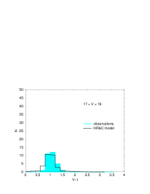
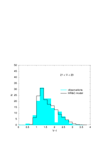
Figure 14: Comparison between the observed (shaded region) and predicted distribution of $V-I$ colours in the labelled intervals of magnitude for the three-component model with Haywood et al. parameters. The thick disk scale height and density are respectively 710 pc and 4.6% of the local disk (see text). The adopted LFs are Wielen et al. (1983) for disk and thick disk and Dahn et al. (1995), completed at bright magnitudes with the LF of M30, for the spheroid component.

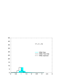
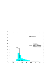
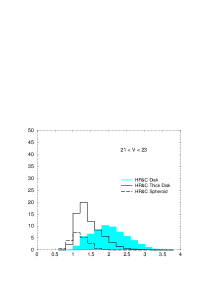
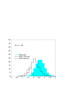
Figure 15: Contributions of the three different populations for the colour-number plots of Fig.14.

Fig. 14 shows the predicted ($V-I$) colour distribution in the labelled intervals of magnitude with the ‘Besancon” parameters tuned as in Fig. 12 with the Wielen et al. LF for the disk and Dahn et al. 1995 (+ M30) LF for the spheroid (heavy long dashed line in Fig.12). Following Gilmore (1984) (see also Reid & Majewski 1993) we used the CMD of the metal rich globular cluster 47 Tucanae to derive the color-magnitude relation for evolved thick disk stars. For MS thick disk stars we used theoretical predictions with Z=0.006 (Cassisi et al. 2000) which, as already discussed, have shown to be in very good agreement with observational data. In all cases E(B-V)=0.18. One sees that the agreement is reasonable in all the magnitude intervals. Figure 15 shows the contribution of disk, thick disk and spheroid to the colour-number plots of Fig.14. Due to the HR&C choice of normalizations, scale heights and scale lenghts, the thick disk contribution in the selected intervals of magnitude is slightly larger than the disk contribution (see Fig. 11). Moreover the thick disk colors are bluer than the disk ones due the lower metallicity (Z=0.006) of the thick disk.

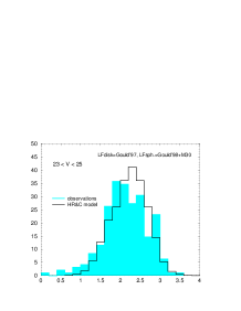
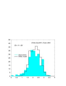
Figure 16: Comparison between the observed (shaded region) and predicted distribution of $(V-I)$ colours for 23$<$V$<$25 for the three component model with Haywood et al. parameters and for different combinations of disk/thick disk/spheroid LFs (as labelled). The thick disk scale height and density are respectively 710 pc and 4.6% of the local disk (see text).

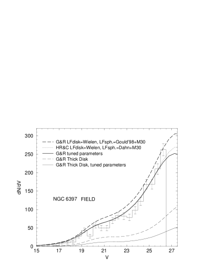
Figure 17: Comparison among theoretical magnitude distribution for the Gilmore & Reid model with original (heavy dashed line) and tuned parameters (heavy solid line, see text). The adopted LFs are Wielen et al. for the disk/thick disk and Gould et al. 98 (+M30) for the spheroid. For comparison the model with the HR&C parameters tuned as in Fig. 12 is also shown (dotted line); the adopted LFs are Wielen et al. for the disk/thick disk and Dahn et al.(+M30) for the spheroid. The thick disk contribution to the total counts is also shown.

Figure 16 compares observed and predicted colour counts for 23$<$V$<$25 for different assumptions about the faint LFs for disk/thick disk and spheroid (see Fig.12 for the corresponding magnitude distributions). As in the two-component model, all the LF combinations taken into account (even Gould et al. 1997 - Gould et al. 1998) show an acceptable fit to observational data; thus the color distributions does not allow to discriminate among different LFs at faint magnitudes.

For the Gilmore & Reid model too the thick disk parameters can be tuned to reconcile the model with observations. In this case one expects that due to the lower contribution of the thick disk to the counts (see Fig.11) the effect of varying the thick disk parameters will be lower. In fact, taking as representative the estimate of errors by Robin et al. (1996), to obtain a good agreement with observational data, one needs to reduce the thick disk scale height and normalization by 2$\sigma$ (scale height=1100 pc, normalization=1.25%). Figure 17 shows the magnitude distribution for the model with original Gilmore & Reid (1983) parameters, (with Wielen et al. disk/thick disk LF and Gould et al., 1998, +M30 spheroid LF) together with the corresponding results when the thick disk parameters are lowered by 2$\sigma$. For comparison the model with the HR&C parameters tuned as in Fig. 12 is also provided. With this modifications the results of the G&R model appear as good as the HR&C one. We do not show the color distributions for the “modified” G&R model because as disclosed by Fig.17, the results are practically coincident with those of Fig.14 and Fig.16.

5 Conclusion

In this paper we have discussed star counts in the field of the globular NGC 6397. As expected, we found that the predicted distribution of stars fainter than M_V$\approx$24 is critically dependent on the assumptions about the LF of faint MS stars. According to the discussion given in the previous sections one finds that neither the two-component B&S model not the more sophisticated three-component models by HR&C and G&R can satisfactory fit star counts in the field of NGC 6397, when assuming for disk and spheroid the low LF suggested by Gould et al. (1997), Gould et al. (1998), respectively. A satisfactory fit of the data can be achieved, either for a two-component or for a three component model, with other suitable combinations of LFs suggested in the current literature, provided that density and scale height of the two discussed three-component models are decreased within the predicted existing uncertainties. Nor the color distributions appear able to discriminate among the various possible solutions. However, we regard the previous conclusions as suggestions to be further tested in deep surveys at different Galactic locations. In this context, and before closing the paper, one has to notice that from the comparison of Figs. 2 and 6 one derives the tantalizing evidence that going deeper than $V$=26.5 by a couple of magnitudes one would derive much more stringent and precise constraints on the LF of faint stars and, in turn, on the mean metallicity of the spheroid. Such an evidence should be taken into account in future researches on this matter.

References

- [1] Anthony-Twarog B.J., Twarog B.A. & Suntzeff N.B., 1992, AJ 103, 1264
- [2] Bahcall J.N. 1986, ARA&A, 24, 577
- [3] Bahcall J.N. & Soneira R.M. 1980, ApJS 44, 73
- [4] Bahcall J.N. & Soneira R.M. 1984, ApJS 55, 67
- [5] Basilio X.S., Gilmore G. & Elson R.A.W., 1996, MNRAS 281, 871
- [6] Bessel M.S. & Brett V.M., 1988, PASP 100, 1134
- [7] Boeshaar P.C. & Tyson J.A., 1985, AJ 90, 817
- [8] Burstein D. & Heiles C., 1982, AJ 87, 1165
- [9] Casertano S., Ratnatunga K.U. & Bahcall J.N., 1990, 357, 435
- [10] Cassisi S., Castellani, V., Ciarcelluti P., Piotto, G., Zoccali M., 2000, MNRAS 315, 679
- [11] Colles M., Ellis R. S., Taylor K. & Shaw G., 1991, MNRAS 253, 686
- [12] Dahn C.C., Liebert J., Harris H.C., Guetter H.H. 1995, in ‘The Bottom of the Main Sequence - And Beyond”, Tinney C.G. ed., ESO workshop, p.239.
- [13] Da Costa G.S., 1982, AJ 87, 990
- [14] Drukier G.A., Fahlmann G.G., Richer H.B., Searle L., Thompson I., 1993, AJ 106, 2335
- [15] Flynn C. & Freeman K.C., 1993, A&AS 97, 835
- [16] Gilmore, G. F., 1981, MNRAS, 195, 183
- [17] Gilmore, G. F., 1984, MNRAS 207, 223
- [18] Gilmore G. F., Wyse R.F.G. & Kuijken K., 1989, ARA&A 27, 555
- [19] Gilmore G. F. & Reid N., 1983, MNRAS 202, 1025
- [20] Gizis J.E. & Reid I.N., 1999, AJ 117,508
- [21] Gould A., Bahcall J.N. & Flynn C. 1996, ApJ 465, 759
- [22] Gould A., Bahcall J.N. & Flynn C. 1997, ApJ 482, 913
- [23] Gould A., Bahcall J.N. & Maoz D., 1993, ApJS 88, 53
- [24] Gould A., Flynn C., Bahcall J.N. 1998, ApJ 503, 798
- [25] Hesser, J. E., Harris, W. E., Vandenberg, D. A., 1987, PASP 99, 1148
- [26] Harris, W.E. 1996, AJ 112, 1487
- [27] Haywood M., Robin A.C. & Creze M., 1997, A&A 320, 440
- [28] Johnson H.L., 1965, ApJ 141, 170
- [29] Johnson H.L., 1966, ARA&A 4, 193
- [30] Johnson J.A. & Bolte M., 1998, AJ 115, 693
- [31] Keenan P.C., 1963, in “Basic Astronomical data” ed. K.A. Strand, Chicago: Univ. Chicago Press, p.78
- [32] King I.R., Anderson J., Cool A.M., Piotto G. 1998, ApJ 492, L37 (KACP)
- [33] Kovalevski J. 1998, ARA&A 36, 99
- [34] Lasker B.M. et al., 1990, AJ 99, 1019
- [35] Martini P. & Osmer P. 1998, AJ 116, 2513
- [36] McCuskey S.W. 1966, in Vistas in Astronomy, edited by A.Beer (Pergamon, Oxford) p.141
- [37] Mendez R.A., Minniti D., De Marchi G., Baker A., Couch W.J., 1996, MNRAS 283, 666
- [38] Mendez R.A. & Guzman R., 1998, A&A 333, 106
- [39] Monet D.G. et al. 1992, AJ 103, 638
- [40] Morgan J.G. & Eggleton P.P, 1978, MNRAS, 182, 219
- [41] Montgomery K.A., Marschall L.A. & Janes K.A., 1993, AJ 106, 181
- [42] Norris J.E. & Ryan S.G., 1991, ApJ 380, 403
- [43] Ojha D.K., Bienayme O., Robin C.A., Creze M., Mohan V., 1996, A&A 311, 456
- [44] Piotto G., Cool A.M. & King I.R. 1997, AJ 113, 1345
- [45] Piotto G. & Zoccali M. 1999, A&A 345, 485
- [46] Ratnatunga K.U. & Bahcall J.N. 1985, ApJS 59, 63
- [47] Reid I.N. & Majewski S.R., 1993, ApJ 409, 635
- [48] Reid I.N. & Gizis J.E., AJ 113, 2246
- [49] Robin A.C. & Créze M., 1986, A&A 157, 71
- [50] Robin A.C., Haywood M., Créze M., Ojha D.K., Bienaymé O., 1996, A&A 305, 125
- [51] Sandage A., 1972, ApJ 178, 1
- [52] Sandage A., 1970, ApJ 162, 841
- [53] Sandquist E.L., Bolte M., Langer G.E., Hesser J.E., Mendes de Oliveira C. 1999, ApJ 518, 262.
- [54] Stuwe, J.A., 1990, A&A 237, 178 & P. Hut (Dordrecht; Reidel) 541
- [55] Wielen R., Jahreiss H., Kruger R. 1983, IAU Coll. 76 ”Nearby Stars and the Stellar Luminosity Function”, A.G.D. Philip ed. (WJK)
- [56] Williams R.E. et al., 1996, AJ 112, 1335
- [57] Wyse R.F. & Gilmore G., 1995, AJ 110, 2771
- [58] Yamagata T. & Yoshii Y., 1992, AJ 103, 117