On formation rate of close binaries consisting of a super-massive black hole and a white dwarf

Abstract

The formation rate of a close binary consisting of a super-massive black hole and a compact object (presumably a white dwarf) in galactic cusps is calculated with help of the so-called loss cone approximation. For a power-law cusp of radius $r_{a}$, the black hole mass $M\sim 10^{6}M_{\odot}$, and the fraction of the compact objects $\delta\sim 0.1$ this rate $\dot{N}_{wd}\sim 4\cdot 10^{-5}K(p)\sqrt{{GM\over r_{a}^{3}}}\approx 3\cdot 10^{-9}K(p){({M\over 10^{6}M_{\odot}})}^{1/2}{({r_{a}\over 1pc})}^{-3/2}yr^{-1}$. The function $K(p)$ depends on parameter $p$ determining the cusp profile, and for the standard cusp profiles with $p=1/4$ $K(p)\sim 2$. We estimate the probability ${\it Pr}$ of finding of a compact object orbiting around a black hole with the period $P$ in one particular galaxy to be ${\it Pr}\sim 10^{-7}{({P/10^{3}s\over M/10^{6}M_{\odot}})}^{8/3}{({M/10^{6}M_{\odot}\over r_{a}/1pc})}^{3/2}$. The object with the period $P\sim 10^{3}s$ emits gravitational waves with amplitude sufficient to be detected by LISA type gravitational wave antenna from the distance $\sim 10^{3}Mpc$. Based on estimates of masses of super-massive black holes in nearby galaxies, we speculate that LISA would detect several such events during its mission.

1 Introduction

A compact object orbiting around a super-massive black hole with mass $\sim 10^{5}-10^{6}M_{\odot}$ with periods $\sim 10^{3}-10^{4}s$ produces gravitational radiation which could be detected by future space-based gravitational antennas. As was mentioned by a number of authors, such object could settle in a tight orbit around the black hole due to combined action of two body gravitational encounters with other stars in galactic centers and emission of gravitational radiation. The gravitational radiation coming from such object yields a direct information about relativistic field of the black hole. Therefore, it is very interesting to estimate the rate of production of close binaries consisting of a super-massive black hole and a compact object (the capture rate below), and the probability ${\it Pr}$ of finding of a galaxy with such a binary in the center. This problem has been investigated before by Hils and Bender 1995 and Sigurdsson and Rees 1997. Hils and Bender performed numerical calculation of the capture rate for a black hole and a central stellar cluster with parameters similar to that was observed in the center of M32. Sigurdsson and Rees (hereafter SR) generalized this result by making estimates of the capture rate for a more general model of the galactic centers. The purpose of this paper is to extend the results obtained before by calculation of the capture rate and the probability ${\it Pr}$ in frameworks of the so-called “loss cone approximation” (e. g. Lightman $\&$ Shapiro 1977, hereafter LS, and references therein). Also, we correct a mistake made in previous estimates.

In what follows we consider a black hole and a stellar cluster around it with parameters close to the parameters of the black hole and the stellar cluster in the center of our own Galaxy. At first, we assume that the black hole mass is about $10^{6}M_{\odot}$. Inside a radius where the black hole mass is approximately equal to the total mass of the stars, a power law increase of the star’s number density with decreasing of distance (called the “cusp” in the stellar distribution) is predicted by theory (e.g. Bahcall and Wolf 1976). Existence of the cusp is in agreement with observations of the center of our Galaxy (e.g Alexander 1999). Based on observations of our Galaxy and other nearby galaxies, we would expect the cusp radius of the order $\sim 1pc$. As it will be clear from our discussion (see the next Section), in order to calculate the capture rate we will be interested in inner regions of the cusps, where the density of normal stars is strongly suppressed by star-star collisions. Therefore, we will be interested in compact objects, which could survive collisions with normal stars. There is also another argument for paying special attention to the compact objects in our problem. Namely, a normal star orbiting around a black hole with period of interest must be tidally disrupted, and therefore only the compact objects with small tidal radii may give a persistent source of gravitational radiation. As it was argued by SR, it it reasonable to suppose that the galactic centers contain evolved population of stars, with a large number of white dwarfs (the ratio of the total number of white dwarfs to the total number of the normal stars $\delta\sim 0.1$). Since the capture rate is proportional to the total number of compact objects, the white dwarfs could yield the main contribution to the capture rate. Therefore, for simplicity, we consider below the innermost part of the cusp consisting purely of white dwarfs. The generalization of our results on the case of neutron stars and solar mass black holes is straightforward.

We calculate the capture rate in Section 2. In Section 3 we estimate the probability ${\it Pr}$. We summarize and discuss our results in Section 4.

G is the Newton constant of gravity and c is the speed of light throughout the Paper. We use expressions from Gradshtein and Ryzhik 1994 when operating with special functions without explicit referencing to that book.

2 Capture rate

For estimate of the capture rate we must compare influence of two body gravitational encounters and emission of gravitational radiation on the orbit of a white dwarf. At first we need a simple model of distribution of normal stars and white dwarfs inside the galactic cusps. As a first approximation we use the standard power law isotropic distribution function of stars in the phase space (e.g Spitzer 1987, Lightman $\&$ Shapiro 1977, hereafter LS)

$$f\approx CE^{p},$$

where $C$ is a constant, $E=GM/r-v^{2}/2$ is the binding energy of a star per unit of mass and $v$ is the velocity of a star. The parameter $p<3/2$ should be rather small from theoretical ground, it has two preferable values: $p=0$ (Peebles 1972, Young 1980) and $p=1/4$ (Bachall and Wolf 1976) . Estimates of this parameter from modeling of stellar distribution in the center of our galaxy made by Alexander 1999 also favor rather small values. The number density of stars is obtained from (1) by integration over the velocity space:

$$n(r)\approx n_{a}({r\over r_{a}})^{-(3/2+p)},$$

where $r_{a}$ is the radius of the cusp and $n_{a}$ is the number density of stars at $r_{a}$. The constant $C$ is related to $n_{a}$ as

$$C=2^{-5/2}\pi^{-1}{({GM\over r_{a}})}^{-(p+3/2)}{n_{a}\over B(3/2;p+1)},$$

where $M$ is the black hole mass and $B(x,y)$ is the Beta function The total mass of stars inside a sphere of radius $r<r_{a}$ is given as

$$M(r)=4\pi\beta mn_{a}r^{3}_{a}{({r\over r_{a}})}^{1/\beta},$$

where $m$ is the star’s mass and

$$\beta={1\over 3/2-p}.$$

As we mentioned in Introduction, the total mass of stars in the cusp must be of order of the black hole mass $M$. In this paper we assume that these two masses are equal: $M(r_{a})=M$. This gives the normalization condition:

$$n_{a}={M\over 4m\pi\beta r_{a}^{3}}.$$

We assign the subscript “wd” to all quantities describing white dwarfs. It is assumed below that the distribution function of white dwarfs $f_{wd}$ has the form analogous to the form of distribution (1), but the total number of white dwarfs $N_{wd}$ is $\delta\sim 0.1$ times smaller than the total number of normal stars $N=M/m$ (SR):

$$f_{wd}\approx\delta CE^{p}$$

All masses of white dwarfs are assumed to be equal to the solar mass $M_{\odot}$, and their radii are equal to $0.01R_{\odot}\approx 7\cdot 10^{8}cm$.

Both distribution functions $f$ and $f_{wd}$ must be strongly modified at sufficiently high energies, where star-star collisions come into play and strongly reduce the number of stars with high binding energy. We would like to take this effect into account in the simplest approximation possible. Therefore, we assume that the distribution function of normal stars is equal to zero at all energies exceeding the cutoff energy

$$E_{coll}\approx{Gm\over R_{star}}=(q{r_{a}\over R_{star}}){GM\over r_{a}},$$

where

$$q=m/M\sim 10^{-6}.$$

Assuming that all normal stars have solar masses and radii, we obtain another useful form of (7)

$$E_{coll}\approx 43(q_{6}r_{1}){GM\over r_{a}},$$

where $q_{6}=m/M_{6}$ and $M_{6}={M\over 10^{6}M_{\odot}}$, $r_{1}=r_{a}/1pc$. The cutoff energy of white dwarfs $E_{coll}^{wd}$ is approximately one hundred times larger than $E_{coll}$:

$$E_{coll}^{wd}\approx 4300(q_{6}r_{1}){GM\over r_{a}}.$$

In our paper we are mainly interested in evolution of angular momentum (per unit of mass) of low angular momentum orbits of stars due to two body gravitational encounters. The change of angular momentum per one orbital period is a random quantity, and its dispersion $j^{2}_{2}$ plays a central role in our analysis. This quantity can be calculated provided the distribution function of stars in the phase space is given (Chandrasekhar 1942, Rosenbluth at al 1957, Cohn $\&$ Kulsrud 1978, Spitzer 1987, Bisnovatyi-Kogan et al and references therein) as a function of orbital parameters of a star (i.e. its binding energy $E$ and its angular momentum $J$). However, in general, it has too complicated form. Therefore, we use several simplifying assumptions when calculating this quantity. 1) The expression (2) is used for the number density of stars in the cusp. 2) $j^{2}_{2}$ is calculated in the low angular momentum limit ($J\rightarrow 0$). 3) We use additional simplification for the distribution function of stars over velocity $F(v)$. Namely, we take $F(v)$ in the form

$$F(v)=3v_{max}^{-3}v^{2},$$

for $v<v_{max}$ and $F(v)=0$ for $v>v_{max}$. Here $v_{max}={({2GM\over r})}^{-3/2}$, and the factor $3v_{max}^{-3}$ in (10) is determined by the normalization condition $\int^{v_{max}}_{0}dvF(v)=1$. Equation (10) is exact for $p=0$. Since we are mainly interested in rather low values of $p$: $0<p<1/4$, the expression (10) is approximately valid for the interesting range of $p$. Even for values of $p\sim 1$, the expression (10) gives an error of order of unity which is insignificant for our purposes (see, however Cohn $\&$ Kulsrud 1978, Shapiro $\&$ Marchant 1978, Young 1980 who use the exact value of this quantity in numerical computations). Under these assumptions we have:

$$j^{2}_{2}={\kappa n_{a}r_{a}^{3/2+p}\over 10GM}{({GM\over E})}^{5/2-p}I(p),$$

where $\kappa=8\pi(Gm)^{2}Ln\Lambda$, $Ln\Lambda\approx Ln(0.5N)$ is the standard Coulomb logarithm. The correction factor

$$I(p)=B(5/2-p;1/2)\{4+{5/2-p\over 3-p}\}$$

weakly depends on $p$: $I(0)=29\pi/6\approx 5.65$ and $I(p=1/4)\approx 5.75$. It is instructive to compare the expression (11) with that was used by LS. LS approximate $F(v)$ to be of the Maxwell form and obtain

$$j^{2}_{2}(LS)={0.501\over 2^{3/2}}\sqrt{(5+2p)}B(5/2-p;1/2){\kappa n_{a}r_{a}^{3/2+p}\over GM}{({GM\over E})}^{5/2-p}.$$

The ratio $R=j^{2}_{2}(LS)/j^{2}_{2}$ has the following values: $R(p=0)=0.82$, $R(p=1/4)=0.86$, $R(p=3/4)=0.95$ and $R(p=1)=0.99$. The deviation introduced by this difference in our final results is absolutely insignificant. However, as we have mentioned above, our expression is exact for $p=0$.

The expression (11) is valid for $E<E_{c}$. In the case $E_{c}<E<E_{c_{w}d}$ this expression is $\delta$ times smaller:

$$j^{2}_{2_{w}d}=\delta j^{2}_{2}=C_{1}q(GMr_{a})\tilde{E}^{p-5/2},$$

where the dimensionless energy variable

$$\tilde{E}={r_{a}E\over GM},$$

and the correction factor

$$C_{1}={\delta Ln\Lambda I(p)\over 5\beta}$$

is of order of unity. We use equations (3), (5), (6) and (11) to obtain (13).

For our purposes we are interested in the innermost part of the cusp, where the number density of normal stars is suppressed due to star-star collisions. Therefore, it is assumed that two body gravitational deflections of a test star are mainly produced by white dwarfs. Generalization of all equations on the case of deflection by normal stars is trivial.

It is very important to note that a black hole is able to capture low angular momentum stars directly (see, e. g. Frolov $\&$ Novikov 1998 and references therein). Hereafter we would like to consider the simplest case of Schwarzschild black hole where the process of direct capture can be described in a very simple way. Namely, the star is captured by a Schwarzschild black hole when its angular momentum $J$ is smaller than the critical angular momentum:

$$J_{crit}={4GM\over c}$$

which defines the size of “loss cone” in the stellar distribution. Therefore, it is very convenient to use the dimensionless quantity

$$x={J\over J_{crit}}$$

instead of $J$ in our analysis. The corresponding dispersion $x^{2}_{2_{w}d}\equiv j^{2}_{2_{w}d}/J^{2}_{crit}$ can be written as

$$x^{2}_{2_{w}d}={C_{1}q\over 4^{2}}({r_{a}c^{2}\over GM}){\tilde{E}}^{p-5/2}.$$

In the simplest approximation influence of two body encounters on the star’s orbit can be described as follows. Let the dimensionless angular momentum of the test star $x$ to walk randomly during some time interval $\Delta t$ due to two body gravitational encounters. Then, the rms value of difference ${<\Delta x>}^{1/2}$ between initial and final values of $x$ is changing with time according to the usual square root law:

$${<\Delta x^{2}>}^{1/2}\sim\sqrt{x^{2}_{2_{w}d}{\Delta t\over P(E)}}$$

where

$$P(E)={\pi GM\over\sqrt{2E^{3}}}=\pi\sqrt{{r_{a}^{3}\over 2GM}}{\tilde{E}}^{-3/2}$$

is the orbital period of the star.

Now let us consider influence of emission of gravitational waves on the star’s orbit. This influence is important for star’s orbits with very high eccentricity $e\approx 1$. Therefore, we can use an approximate expression for the orbit decay time-scale $T{gw}$ obtained by Peters 1964 in the limit of highly eccentric orbits:

$$T{gw}={3\over 85}{c^{5}\over GM}q^{-1}a^{4}(1-e^{2})^{7/2},$$

where $a={GM\over 2E}$ is the major semi-axis and $e$ is the eccentricity. Using the standard expressions of celestial mechanics we can express $T_{gw}$ in terms of variables $x$ and $\tilde{E}$:

$$T{gw}={3\cdot 4^{7}\over 85\sqrt{2}}q^{-1}({GM\over c^{2}r_{a}})(x^{7}{\tilde{E}}^{-1/2})\sqrt{{r_{a}^{3}\over GM}}.$$

As one can see, $T_{gw}$ sharply decreases $\sim x^{7}$ with decrease of $x$.

A star has a considerable probability to be captured on a highly bound orbit when its angular momentum $x$ is smaller than the size of “gravitational wave loss cone” (see also SR) defined as

$$x_{gw}=\sqrt{x^{2}_{2_{w}d}{T_{gw}(x_{gw})\over P(E)}}.$$

Using equations (17,19), we obtain

$$x_{gw}={1\over 4}{({85\pi\over 3C_{1}})}^{1/5}{\tilde{E}}^{1\over 5\beta}\approx{0.6\over C_{1}^{1/5}}{\tilde{E}}^{1\over 5\beta}.$$

Action of two body gravitational encounters and emission of gravitational waves changes the distribution function $f_{wd}(x,\tilde{E})$. To find this change, one can use the standard Fokker-Plank approach to the problems of stellar dynamics (e.g. Spitzer 1987 and references therein). However, the Fokker-Plank equation must be properly modified to take into account emission of gravitational waves. It is easy to see that the stationary variant of the modified equation should have the form:

$${\partial\over\partial E}({\dot{E}_{gw}}{\cal N}_{wd})+{\partial\over\partial J}({\dot{J}_{gw}}{\cal N}_{wd})=\hat{F}_{F-P}({\cal N}),$$

Here

$${\cal N}_{wd}=8\pi^{2}f_{wd}P(E)J$$

is the distribution function of white dwarfs over energy and angular momentum. It is normalized by the condition: $\int dEdJ{\cal N}_{wd}=N_{wd}$. $\dot{E}_{gw}(E,J)$ and $\dot{J}_{gw}(E,J)$ are, respectively, the rate of change of binding energy and angular momentum of a particular star due to emission of gravitational waves. Explicitly, $\dot{E}_{gw}(E,J)$ and $\dot{J}_{gw}(E,J)$ were calculated by Peters 1964. $\hat{F}_{F-P}$ is the standard Fokker-Plank operator. We need below only the expression for $\dot{E}_{gw}(E,J)$:

$$\dot{E}_{gw}={85\over 3\cdot 4^{7}x^{7}}qc^{2}\sqrt{{GM\over r_{a}^{3}}}{\tilde{E}}^{3/2}.$$

In general, equation (24) is too complicated to be solved analytically. However, we can make several simplifying assumptions. Namely, we use the standard approximations of the loss-cone theory (e.g. LS) neglecting differentiation over energy in the Fokker-Plank operator and considering the diffusion coefficients in the low angular momentum limit. In this limit, the right hand side of (24) takes the form:

$$4\pi^{2}j^{2}_{2_{w}d}{\partial\over\partial J}J{\partial\over\partial J}f_{wd}.$$

Next, we can neglect the term ${\partial\over\partial J}({\dot{J}_{gw}}{\cal N}_{wd})$ on the left hand side of (24). Indeed, this term is $\sim E/c^{2}$ times smaller than the leading term ${\partial\over\partial E}({\dot{E}_{gw}}{\cal N}_{wd})$.

After these assumptions being accepted, equation (24) is reduced to a parabolic type equation

$${\partial\over\partial E}({\dot{E}_{gw}}P(E){f}_{wd})={j^{2}_{2_{w}d}\over 2J}{\partial\over\partial J}J{\partial\over\partial J}f_{wd},$$

Substituting (19,26) in (28), we obtain

$${85\sqrt{2}\pi\over 3\cdot 4^{5}C_{1}}{\tilde{E}}^{5/2-p}{\partial\over\partial\tilde{E}}f_{wd}=x^{6}{\partial\over\partial x}x{\partial\over\partial x}f_{wd}.$$

This equation should be solved with the outer boundary condition

$$f_{wd}(E,J_{max})=\delta CE^{p},$$

where $J_{max}={GM\over\sqrt{2E}}$ is the angular momentum of a circular orbit. Instead of $J_{max}$ we use below the corresponding dimensionless angular momentum:

$$x_{max}={J_{max}\over J_{crit}}={1\over 4}{({c^{2}r_{a}\over 2GM})}^{1/2}{\tilde{E}}^{-1/2}.$$

The condition of absorbing wall

$$f_{wd}(x=1)=0$$

can be imposed as an approximate inner boundary condition.

Equation (29) should be solved separately for the degenerate case $p=0$ and for the general case $p>0$. At first let us consider the case $p=0$. For this case the “stationary” solution (${\partial\over\partial\tilde{E}}f_{wd}=0$) is compatible with the boundary conditions (30) and (32). This solution has the standard form (e.g LS, Cohn $\&$ Kulsrud 1978):

$$f_{wd}=Aln(x),$$

where the normalization constant $A$ can be determined from the outer boundary condition. The value of the distribution function at $x=x_{max}$:

$$f_{wd}(x=x_{max})=Aln({J_{max}\over J_{crit}})=Aln({1\over 4}{({c^{2}r_{a}\over 2GM})}^{1/2}{\tilde{E}}^{-1/2})$$

depends logarithmically on energy, and therefore it cannot be directly equated to (30). Therefore, we equate the last expression and (30) at some fixed energy $E_{*}$ which is specified below (see equation (40)). Similar to the usual loss cone theory (LS), this leads to slow logarithmic dependence of the effective power $p_{eff}\equiv{dln(f_{wd})\over dln(x)}$ of the distribution function on energy. By this way we obtain the normalization constant in the form:

$$A={\delta C\over ln\Lambda_{2}},$$

where

$$ln\Lambda_{2}=ln({1\over 4}{({c^{2}r_{a}\over 2GM})}^{1/2}E_{*}^{-1/2}).$$

The constant $C$ in (34) is calculated with help of (3),(5):

$$C={2^{-13/2}9\pi^{-2}q^{-1}\over{(GMr_{a})}^{3/2}}.$$

For $p=0$ the flow of white dwarfs toward larger energies

$$\dot{N}^{0}_{wd}\equiv\int^{J_{max}}_{J_{crit}}dJN_{wd}\dot{E}_{gw}$$

does not depend on energy. It is calculated with help of (3), (5,6), (25,26),(33,34):

$$\dot{N}^{0}_{wd}={51\pi\over 5\cdot 4^{7}}{\delta\over ln\Lambda_{2}}\sqrt{{GM\over r_{a}^{3}}}.$$

For small energies only a small fraction of white dwarfs can be carried toward sufficiently large energies by $\dot{N}_{wd}$, and the main fraction is absorbed by the absorbing wall at $x=1$. Alternatively, at large energies, almost all white dwarfs diffused to small angular momenta of order of $x_{gw}$ form the flow $\dot{N}_{wd}$. It is reasonable to identify the boundary between the small and large energies as the energy $E_{*}$ where the logarithm (35) is evaluated. To find $E_{*}$ we calculate the diffusion flow per unit of energy:

$${d\dot{N}_{diff}\over dE}=4\pi^{2}j^{2}_{2_{w}d}J{\partial f_{wd}\over\partial J}={2^{-9/2}C_{1}\delta\over{(GMr_{a})}^{1/2}}{\tilde{E}}^{-5/2}.$$

The condition

$$\int^{\infty}_{E_{*}}d\dot{N}_{diff}=\dot{N}^{0}_{wd}$$

gives an implicit equation for $E_{*}$. This equation has an approximate solution

$$E_{*}\approx 72{({ln\Lambda_{2}C_{1}\over 4.5})}^{2/3},$$

and

$$ln\Lambda_{2}\approx 4.5+0.5ln({70\over E_{*}}{r_{1}\over M_{6}}),$$

where $r_{1}=r_{a}/1pc$ and $M_{6}=M/M_{\odot}$. It is important to note that the energy $E_{*}$ is of order of the “collision” cutoff energy $E_{coll}$ for the normal stars (see eq. (8)), but much smaller than the “collision” cutoff energy $E^{wd}_{coll}$ for the white dwarfs (eq. (9)). Thus, our assumption of absence of the normal stars at energies of interest is fulfilled.

Now let us consider the general case $p>0$.

Before solving equation (29) for $p>0$, let us point out that this equation can be brought into a standard form by the following change of variables:

$$y=x^{-5/2},\quad\tau=C_{2}{\tilde{E}}^{-1/\beta},$$

where

$$C_{2}\approx{15\cdot 4^{4}C_{1}\beta\over 17\sqrt{2}\pi}\approx 159,7C_{1}\beta.$$

We have

$${\partial\over\partial\tau}f_{wd}+{1\over y}{\partial\over\partial y}y{\partial\over\partial y}f_{wd}=0.$$

Obviously, equation (43) is the standard diffusion equation written in cylindrical coordinates, but with negative and constant coefficient of diffusion. A formal general solution to (43) can be written as:

$$f_{wd}=A\int^{\infty}_{0}d\lambda D(\lambda)e^{-\lambda\tau}\Psi(y),$$

where the function $\Psi(y)$ satisfies the Bessel equation for the zero index Bessel functions of imaginary argument:

$${1\over y}{d\over dy}y{d\over dy}\Psi-\lambda\Psi=0.$$

Now we would like to construct the solution to (43) satisfying the boundary conditions (30) and (32). At first, formally assuming that the size of “gravitational wave loss cone” $x_{gw}$ is much larger than unity we look for a self-similar solution to (43). For this solution the inner boundary condition is reduced to the condition of that $f_{gw}$ decreases with decrease of $x$. The McDonald function $K_{0}(z)$ decreases with increase of the argument, and hence the self-similar solution to (43) must be proportional to $K_{0}(\lambda^{1/2}y)$. We choose the function $D(\lambda)$ to be

$$D(\lambda)=\lambda^{\beta p-1},$$

and obtain:

$$f^{ss}_{wd}=A\int^{\infty}_{0}d\lambda\lambda^{\beta p-1}e^{-\lambda\tau}K_{0}(\lambda^{1/2}y).$$

It is easy to see that the solution (47) has a self-similar form indeed. For that let us change the integration variable in (47): $\tilde{\lambda}=\lambda\tau$, and introduce the self-similar coordinate:

$$\xi={y\over\tau^{1/2}}.$$

We have

$$f_{wd}=\tilde{A}{\tilde{E}}^{p}\int^{\infty}_{0}d\tilde{\lambda}{\tilde{\lambda}}^{\beta p-1}e^{-\tilde{\lambda}}K_{0}({\tilde{\lambda}}^{1/2}\xi),$$

where $\tilde{A}={A\over C_{2}^{\beta p}}$. The integral in (49) is proportional to the Whittaker function $W_{\mu,0}(z)$:

$$\int^{\infty}_{0}d\tilde{\lambda}{\tilde{\lambda}}^{\beta p-1}e^{-\tilde{\lambda}}K_{0}({\tilde{\lambda}}^{1/2}\xi)=\Gamma^{2}(\beta p){e^{\xi^{2}/8}\over\xi}W_{{1\over 2}-\beta p}({\xi^{2}\over 4}).$$

It is important to note that the self-similar coordinate $\xi$ defines a scale in the angular momentum space of order of $x_{gw}$:

$$\xi={({x\over x_{*}})}^{-5/2},$$

where

$$x_{*}={\tau}^{-1/5}={1\over 4}{({68\sqrt{2}\pi\over 15C_{1}\beta})}^{1/5}{\tilde{E}}^{1\over 5\beta}\approx{0.46\over{(C_{1}\beta)}^{1/5}}{\tilde{E}}^{1\over 5\beta}.$$

Let us discuss the asymptotic behavior of (49). For large $\xi$ (small $x$) we use the approximate asymptotic expression for the Whittaker function

$$W_{\mu,0}(z)\approx z^{\mu}e^{-z/2},$$

to obtain

$$f^{ss}_{wd}\approx{1\over 2}{(4C_{2})}^{\gamma}\tilde{A}\Gamma^{2}(\gamma)x^{5\gamma},$$

where $\gamma=\beta p$. As it is seen from (53), the function $f^{ss}_{wd}$ has a constant nonzero value at $x=1$. This contradicts to the inner boundary condition (32). However, we can subtract this value from $f^{ss}_{wd}$ and satisfy the boundary condition. We have:

$$f_{wd}=f_{wd}^{ss}-f^{ss}_{wd}(x=1)=\tilde{A}\Gamma^{2}(\gamma)\times$$

$$\times\{{\tilde{E}}^{p}{e^{\xi^{2}/8}\over\xi}W_{1/2-\gamma,0}({\xi^{2}\over 4})-{{(4C_{2})}^{\gamma}\over 2}\}.$$

In the limit of small $\xi$ the function (54) has the form (see Appendix):

$$f_{wd}\approx\tilde{A}\Gamma(\gamma){\tilde{E}}^{p}\times$$

$$\times\{ln(2\xi^{-1})-(C_{e}+\psi(\gamma)/2)-\Gamma(\gamma){{(4C_{2})}^{\gamma}\over 2}{\tilde{E}}^{-p}\},$$

where $C_{e}\approx 0.577$ is the Euler constant, and $\psi(z)={d\over dz}ln\Gamma(z)$. The expression (55) is used for normalization of the distribution function (54). Similar to the case $p=0$, $f_{wd}(x=x_{max})$ is not an exact power law function of energy, and we should find the normalization constant $\tilde{A}$ at some fixed energy $E_{*}$. It is reasonable to identify this energy as the energy corresponding to the “time” $\tau=1$ (see equation (41)):

$$E_{*}=C_{2}^{\beta}.$$

Taking into account (41), (48) and (55), we obtain

$$f_{wd}(x=x_{max})(\tilde{E}=E_{*})=\tilde{A}\Gamma(\gamma){\tilde{E}}^{p}\times$$

$$\times\{ln(2x_{max}^{5/2})-(C_{e}+\psi(\gamma)/2+4^{\gamma}\Gamma(\gamma)/2)\}.$$

The last term in the brackets could be important if only $\gamma\rightarrow 0$, where we approximate

$$\psi(\gamma)/2+4^{\gamma}\Gamma(\gamma)/2\approx ln(4).$$

Using equations (30,31) and (56,57), we obtain the normalization constant in the form

$$\tilde{A}={\delta C\over\Gamma(\gamma)ln\Lambda_{3}}{({GM\over r_{a}})}^{p},$$

where

$$ln\Lambda_{3}=ln({e^{-C_{e}}\over 32}{({c^{2}r_{a}\over 2GM})}^{5/4}{\tilde{E}_{*}}^{-5/4})\approx$$

$$11+ln\{{({r_{1}\over M_{6}})}^{5/4}C_{2}^{\beta(1/4-p)}\}.$$

Note, that equations (55) and (58) tell that the “effective power” of the distribution $f_{wd}$ differs from the parameter $p$ on value of order of 0.1. It is also important to point out that the solution (54) satisfies the boundary conditions in the limit $\tau\rightarrow 0$ (e.g $\tilde{E}\gg E_{*}$). We assume below that the solution (54) also gives a reasonable approximation for the moderate values of $\tilde{E}$: $\tilde{E}\geq E_{*}$. For $\tau>1$ ($\tilde{E}<E_{*}$) the effects of gravitational radiations are negligible and we can use the standard solution (33).

Now let us calculate the capture rate of white dwarfs for the case $p>0$. At first it is convenient to calculate the capture rate of white dwarfs due to emission of gravitational waves per unit of energy:

$${d\dot{N}_{wd}\over dE}\equiv\int^{J_{max}}_{J_{crit}}dJ{\partial\over\partial E}(N_{wd}\dot{E}_{gw})$$

This quantity can be expressed as the difference between the diffusion flow of the stars at large values of $x$ and the diffusion flow at $x=1$:

$${d\dot{N}_{wd}\over dE}={d\dot{N}_{diff}\over dE}|_{x\rightarrow x_{max}}-{d\dot{N}_{diff}\over dE}|_{x=1},$$

where

$${d\dot{N}_{diff}\over dE}=4\pi^{2}j^{2}_{2_{w}d}J{\partial\over\partial J}f_{wd}.$$

We calculate the diffusion flows with help of (13), (53,55):

$${d\dot{N}_{diff}\over dE}|_{x\rightarrow x_{max}}=10\pi^{2}j^{2}_{2_{w}d}{\delta C{\tilde{E}}^{p}\over ln\Lambda_{3}}{({GM\over r_{a}})}^{p},$$

and

$${d\dot{N}_{diff}\over dE}|_{x=1}=10\pi^{2}j^{2}_{2_{w}d}\gamma 4^{\gamma}\Gamma(\gamma){\delta C\over ln\Lambda_{3}}{({GM\over r_{a}})}^{p}.$$

Note that the diffusion flow at large $x$ (equation 63) is close to the similar expression obtained by LS in frameworks of “one dimensional” loss cone theory. Substituting (63), (64) in (61), and using (3-5), we obtain:

$${d\dot{N}_{wd}\over dE}=2^{-7/2}{5\delta C_{1}\over\beta B(3/2;p+1)ln\Lambda_{3}}\times$$

$$\times\{{\tilde{E}}^{2p-5/2}-\gamma 4^{\gamma}\Gamma(\gamma)E^{p}_{*}{\tilde{E}}^{p-5/2}\}{1\over{(GMr_{a})}^{1/2}}$$

The total capture rate of white dwarfs can be expressed as

$$\dot{N}_{wd}\approx\int^{E^{wd}_{coll}}_{E_{1}}d\dot{N}_{wd}+\dot{N}^{0}_{wd},$$

where we use equation (37) for $\dot{N}^{0}_{wd}$ and the energy scale

$$E_{1}={(\gamma 4^{\gamma}\Gamma(\gamma))}^{1/p}E_{*}$$

is defined by the condition ${d\dot{N}_{wd}\over dE}(E_{1})=0$. Explicitly integrating (66) and using (42), (56), (67) we have:

$$\dot{N}_{wd}\approx{17\pi\over 6\cdot 4^{6}}({p-(3/2-p)\epsilon^{3/2-2p}+(3/2-2p)\epsilon^{3/2-p}\over 3/2-2p})\times$$

$$\times{{(\gamma\Gamma(\gamma))}^{-1/\gamma}\delta\over\beta B(3/2;p+1)ln\Lambda_{3}}E_{1}^{p}\sqrt{{GM\over r_{a}^{3}}}+\dot{N}_{wd}^{0},$$

where $\epsilon={E_{1}\over\tilde{E}^{wd}_{coll}}\leq 1$. This expression can be rewritten as

$$\dot{N}_{wd}\approx K(p)\dot{N}_{wd}^{0},$$

where

$$K(p)=1+{20\over 18}({p-(3/2-p)\epsilon^{3/2-2p}+(3/2-2p)\epsilon^{3/2-p}\over 3/2-2p})\times$$

$$\times{{(\gamma\Gamma(\gamma))}^{-1/\gamma}ln\Lambda_{2}\over\beta B(3/2;p+1)ln\Lambda_{3}}E_{1}^{p}.$$

The function $K(p)$ is plotted in Fig. (1) for $ln\Lambda=ln(0.5\cdot 10^{5})\approx 11$, $ln\Lambda_{2}=4.5$, $ln\Lambda_{3}=11$, and $\delta=0.1$.

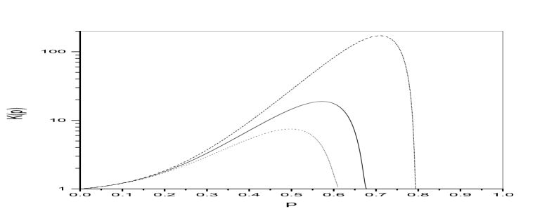
Figure 1: The ratio $K(p)={\dot{N}_{wd}\over\dot{N}^{0}_{wd}}$ is shown as a function of $p$. Solid curve corresponds to $q_{6}r_{1}=1$ and $E_{coll}^{wd}=4300$. Dashed and dotted curves correspond to $q_{6}r_{1}=5$ ( $E_{coll}^{wd}=21500$) and $q_{6}r_{1}=0.5$ ($E_{coll}^{wd}=2150$), respectively. The solid curve has a maximum at $p\approx 0.57$.

One can see from this Fig. that the capture rate depends non-monotonically on $p$, it has a maximum at $p\approx 0.57$ ($K(p=0.57)\sim 19$), for larger values of $p$ our assumption of absence of the white dwarfs at energies larger than $E_{coll}^{wd}$ leads to suppression of the capture rate (see also Fig. 2). The capture rate is mainly determined by stars with “initial” energy

$$E_{in}={({3/2-p\over 3/2-2p})}^{1/p}E_{1},$$

defined by the condition ${d\over dE}({d\dot{N}_{wd}\over dlnE}(E_{in}))=0$ and these stars have their “initial” angular momentum of order of

$$x_{in}=x_{*}(E_{in}).$$

We show the dependence of $E_{in}$ and $x_{in}$ on $p$ in Fig. 2 and Fig 3, respectively.

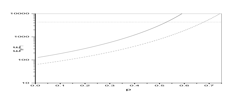
Figure 2: The characteristic energies $E_{in}$ (solid curve) and $E_{1}$ (dashed curve) are shown as functions of $p$. They monotonically increase with $p$. For $p>0.53$ $E_{in}$ is larger than $E^{wd}_{coll}=4300$ (dotted line), and for $p>0.675$ $E_{1}$ is larger than $E^{wd}_{coll}$.

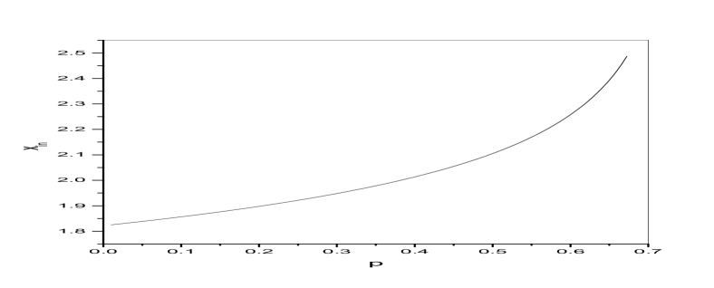
Figure 3: The characteristic angular momentum $x_{in}$ is shown as a function of $p$. It has the value $\approx 1.8$ for $p=0$ and monotonically increases with $p$. For specially important $p=1/4$ $x_{in}\approx 2$.

It is instructive to compare the capture rate obtained in this paper with that was obtained by SR. The ’diffusion’ capture rate of SR can be written as

$$\dot{N}^{SR}(r)\approx 5{({N_{wd}(r)m_{wd}\over M})}^{8/5}({r_{s}\over r})P^{-1},$$

where $r_{s}={2GM\over c^{2}}$, and $N_{wd}$ is the number of white dwarfs within the sphere of radius $r$. In order to describe the spatial scale SR use the radial coordinate $r$ while we work with the energy coordinate $E$. Since the stars spend most of their time near their apocenters $r_{ap}=GM/E$, it is reasonable to use the following rule of change of variables: $r=r_{ap}$. Using equations (4,19) and definition of $\delta$, we have

$$\dot{N}^{SR}(r)\approx{5\sqrt{2}\over\pi}\delta^{8/5}({r_{s}\over r_{a}}){({r\over r_{a}})}^{-(1/10+8p/5)}\sqrt{{GM\over r_{a}^{3}}}={5\sqrt{2}\over\pi}\delta^{8/5}({r_{s}\over r_{a}}){\tilde{E}}^{(1/10+8p/5)}\sqrt{{GM\over r_{a}^{3}}}.$$

One can see from this equation that $\dot{N}^{SR}$ grows with energy, and therefore we use the ’cutoff’ energy $E^{wd}_{coll}$ (equation 9) to obtain the total rate

$$\dot{N}^{SR}\approx 6\cdot 10^{-9}{M_{6}\over r_{1}}\delta_{1}^{8/5}{(\tilde{E}^{wd}_{coll})}^{8p/5+1/10}\sqrt{GM\over r_{a}^{3}},$$

where $\delta_{1}=10\delta$. We show the ratio $R=\dot{N}^{SR}/\dot{N}_{wd}$ in Fig 4.

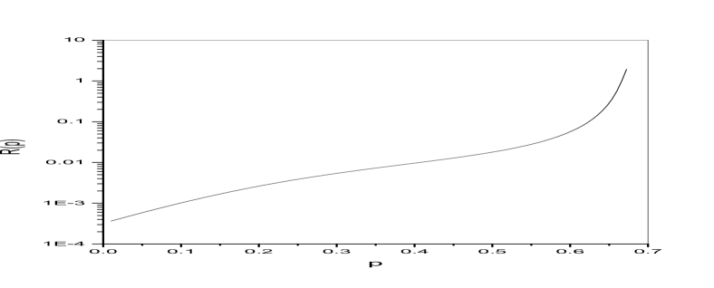
Figure 4: The ratio $R=\dot{N}^{SR}/\dot{N}_{wd}$ is shown as a function of $p$.

One can see that the capture rate of SR is much smaller than our capture rate for small values of $p$ ($\dot{N}^{SR}(p=0)/\dot{N}_{wd}(p=0)\approx 3\cdot 10^{-4}$ and $\dot{N}^{SR}(p=1/4)/\dot{N}_{wd}(p=1/4)\approx 10^{-2}$) . Here we would like to note that SR also obtain the capture rate due to large angle deflections of stars which is several times larger (for the case $p=0$) than our capture rate. The large angle deflections of the stars cannot be treated in framework of the Fokker-Plank approach and are beyond of the scope of this paper.

Finally, let us represent the capture rate in astrophysical units:

$$\dot{N}_{wd}\approx 3\cdot 10^{-9}K(p)\delta_{1}({4.5\over ln\Lambda_{2}}){M_{6}^{1/2}\over r_{1}^{3/2}}yr^{-1},$$

This expression can be directly compared with Monte Carlo simulations made by Hils and Bender 1995 for $p=0$. Hils and Bender obtained the capture rate $\dot{N}^{HB}_{wd}\approx 1.9\cdot 10^{-8}yr^{-1}$ which is $6.3$ times larger than our value. Unfortunately, Hils and Bender did not publish details of their method, and analysis of this disagreement is not possible.

3 Probability of finding of the source of gravitational waves

The probability ${\it Pr}$ of finding of a galaxy with a white dwarf orbiting around central black hole and emitting gravitational radiation in a detectable amount can be defined as

$${\it Pr}=T^{f}_{gw}\dot{N}^{wd},$$

where $T^{f}_{gw}$ is the decay time of an orbit of a white dwarf which is sufficiently close to the black hole to yield a significant amplitude of gravitational waves. Clearly, this time depends not only on physical conditions inside the galactic cusps, but also on properties of gravitational wave antenna receiving the signal, in particular, on frequency band available for such antenna. Therefore, we assign the superscript $f$ to $T^{f}_{gw}$. In particular, the maximal sensitivity of LISA gravitational wave antenna will be in the frequency range $10^{-3}Hz\leq f\leq 10^{-1}Hz$, and sharply decreases with decreasing frequency . LISA would be able to detect a gravitational wave with amplitude $h$ of the order $\sim 10^{-23}$ at $f\sim 10^{-3}Hz$ with a signal-to-noise ratio $\sim 5$. For moderately eccentric orbits the frequency of gravitational waves is inversely proportional to the period $f\sim 1/P(E)$, and therefore we are interested in periods $P(E)$ of order of $10^{3}s$. For such periods and black hole masses, $\sim 10^{6}M_{\odot}$ the semi-major axis $a$ of the orbit is close to five gravitational radii:

$$a=10{({P_{3}\over M_{6}})}^{2/3}{GM\over c^{2}},$$

where $P_{3}={P(E)\over 10^{3}s}$. In such situation, strictly speaking, one should use relativistic expressions for $T^{f}_{gw}$ and other quantities of interest. However, the relativistic expressions are rather complicated, and we are going to use expressions calculated in the Newtonian approximation assuming that this would not significantly alter our order-of-magnitude estimates.

Now we would like to discuss the following problem. Suppose that white dwarfs are supplied on highly eccentric orbits with the rate given by equation (69) and with energy and angular momentum given by equations (71,72). After that the orbital parameters are changed only due to emission of gravitational radiation. What is the eccentricity of the orbit when its period is of order of $10^{3}s$? This problem can be solved with help of relation between parameters of the orbit evolving due to emission of gravitational radiation (Peters 1964):

$$x(e)\approx 0.94x_{in}e^{6/19}H(e),$$

where

$$H(e)={(1+{121\over 304}e^{2})}^{435/2299}$$

slowly changes with $e$. We can rewrite equation (77) as

$$a\approx 14.8{GM\over c^{2}}x_{in}^{2}e^{12/19}H^{2}(e),$$

substitute (76) into (78), and obtain an implicit equation for the eccentricity $e$. Solution of this equation depends parametrically on $p$ (through the dependence of $x_{in}$ on $p$, equation (72)), and also on the ratio $({P_{3}\over M_{6}})$. This solution is shown in Fig. 5.

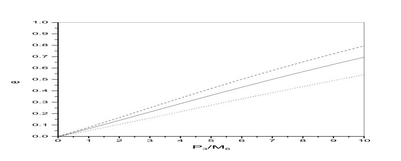
Figure 5: Dependence of the eccentricity $e$ on the ratio $P_{3}/M_{6}$. Solid curve corresponds to $p=1/4$, dashed and dotted curves correspond to $p=0$, $p=0.5$, respectively. Note that these curves are close to straight lines.

As it is seen from this Fig., for the most interesting case $({P_{3}\over M_{6}})\sim 1$, the eccentricity is small ($e\leq 0.1$). Therefore, we neglect the dependence of the decay time $T^{f}_{gw}$ on the eccentricity and use $T^{f}_{gw}$ calculated by Peters 1964 for circular orbits:

$$T^{f}_{gw}={5\over 256}q^{-1}{({ac^{2}\over GM})}^{4}{GM\over c^{3}}\approx 31M_{6}{({P_{3}\over M_{6}})}^{8/3}yr.$$

Substituting (74) and (79) into equation (75) we finally have:

$${\it Pr}\approx 10^{-7}K(p)\delta_{1}({4.5\over ln\Lambda_{2}}){({M_{6}\over r_{1}})}^{3/2}{({P_{3}\over M_{6}})}^{8/3}.$$

Note that ${\it Pr}$ strongly depends on the ratio $P_{3}/M_{6}$.

4 Conclusions

We calculate the formation rate of a close binary in galactic cusps (the capture rate) consisting of a super-massive black hole and a compact object (presumably a white dwarf). We also calculate the probability ${\it Pr}$ to find a galaxy with such a binary emitting gravitational radiation at frequency $f\sim 10^{-3}Hz$. We take into account two main process determining the capture rate: 1) two-body gravitational encounters of the compact object, 2) energy loss due to emission of gravitational radiation, and calculate the capture rate analytically, in frameworks of the so-called loss cone approximation. Our main results are given by equations (37),(69) and (80). These equations explicitly show the dependence of the capture rate and probability ${\it Pr}$ on main parameters of galactic cusps: their radii, the relative number of compact objects in them, the “sharpness” $p$ of increase of the number density of compact objects toward the center of a galaxy and the frequency band of gravitational wave antenna receiving the signal. They could be easily used for estimates of the capture rate and probability ${\it Pr}$ for a broad range of the main parameters. We correct a mistake made by previous researchers in estimate of the capture rate. Our results are obtained in assumption of power law cusps with density $n\sim r^{-(3/2+p)}$. However, generalization of our results on more realistic cusp profiles (say, with different powers $p$ in the outer and inner regions of the cusp, e.g Alexander 1999) is straightforward.

Unfortunately, not so much is known about galactic cusps from observations. Therefore, our results should be considered as qualitative only. Also, much more robust estimates could be obtained using modern computational methods. However, our simple analytical approach clearly shows the dependence on parameters, and therefore, could be used as a guidance for choice of parameters for numerical studies.

In their recent review of black holes found in the galactic centers, Kormendy and Gebhardt 2001 identify three black hole with masses of order of $\sim 10^{6}M_{\odot}$ (one of them is in our own Galaxy) with distance smaller than $13,2Mpc$. Therefore, it seems reasonable to estimate the density of potential sources of gravitational radiation as $\geq 10^{-3}Mpc^{-3}$ . Assuming that we need $\sim 10^{7}$ potential sources to observe at least one event (equation (80)), we need the sensitivity of gravitational wave antenna to be sufficient to detect a source at the distance $D\geq 10^{3}Mpc$. The dimensionless amplitude of a gravitational wave coming from a white dwarf orbiting around a black hole with period $\sim 10^{3}s$ at the distance $\sim 10^{3}Mpc$ from an observer is of order of $10^{-23}$. This amplitude could be easily detected by a gravitational wave antenna of LISA type. Therefore, we could optimistically expect several events during the life-time of LISA mission $\sim 3yr$. Relativistic effects (e.g. influence of Einstein precession and Lense-Thirring precession for a rotating black hole on the shape of the signal) may help to distinguish these events from other sources of gravitational radiation.

Appendix A

It is rather difficult to find decomposition of the Whittaker function $W_{\mu,0}(z)$ for small values of $z$ in the standard reference books on special functions. Therefore, we write below the formulae which are used to obtain (55) from (54).

We use decomposition of the McDonald function for small $z$:

$$K_{0}(z)\approx ln({2\over z})-C_{e},$$

the representation of the Gamma function:

$$\Gamma(z)=\int^{\infty}_{0}d\lambda\lambda^{z-1}e^{-\lambda},$$

and the consequence of (A3):

$$\psi(z)\equiv{d\over dz}ln\Gamma(z)={1\over\Gamma(z)}\int^{\infty}_{0}d\lambda\lambda^{z-1}e^{-\lambda}ln\lambda.$$

References

- [1] Alexander T., 1999, ApJ, 527, 835
- [2] Bahcall J. N., Wolf R. A., 1976, ApJ, 209, 214
- [3] Bisnovatyi-Kogan G. S., Churaev R. S., Kolosov B. I., 1982, AA, 113, 179
- [4] Chandrasekhar, S., 1942, Principles of Stellar Dynamics, Chicago, University of Chicago Press
- [5] Cohn H., Kulsrud R. M., 1978, ApJ, 226, 1087
- [6] Frolov V. P., Novikov I. D., 1998, Black hole physics: basic concepts and new developments, Dordrecht: Kluwer Academic
- [7] Gradshtein I. S., Ryzhik I. M., 1994, Table of Integrals, Series and Products, Academic Press
- [8] Gurevich A. V., Geomagnetism and Aeronomy, 1964, 4, 192
- [9] Hils D., Bender P. L., 1995, ApJ, 445, L7
- [10] Kormendy J., Gebhardt K., 2001, in: The 20th Texas Symposium on Relativistic Astrophysics, ed. H. Martel and J. C. Wheeler, AIP
- [11] Lightman A. P., Shapiro S. L., 1977, ApJ, 211, 244
- [12] Peters P. C., 1964, 136, 1224
- [13] Peebles, P. J. E., 1972, ApJ, 178, 371
- [14] Rosenbluth M. N., MacDonald W. M., Judd D. L., 1957, Rep. Mod. Phys., 107, 1
- [15] Shapiro, S. L., Marchant, A. B., 1978, ApJ, 225, 603
- [16] Sigurdsson S., Rees M. J., 1997, MNRAS, 284, 318
- [17] Spitzer L., 1987, Dynamical evolution of globular clusters, Princeton, NJ, Princeton University Press
- [18] Young P., 1980, ApJ, 249, 1232