Interpreting The ${\rm\bf N_{HI}}$ Power Spectrum

Abstract

In this paper I investigate what factors – both observational and physical – can change the measured slope of the observed 21cm HI power spectrum. The following effects can make the observed turbulence appear two dimensional rather than three dimensional: 1) if the turbulence is contained in a thin filament or slab; 2) if the medium has a high optical depth; and 3) if any method of observation or analysis is used which effectively limits the emission from the medium under study to a thin slab, for example, by analyzing an individual channel map. Straightforward analysis of data can give misleading or incomplete results if these effects are not taken into account.

NRAO, P.O. Box 2, Green Bank, WV 24944

1. Introduction

The 21cm HI line has a column density power spectrum whose slopes are consistent with 2–Dimensional turbulence ($\alpha\sim-8/3$) on large spatial scales ($>0.01$ pc) and narrow velocity ranges (Green 1993; Dickey & Crovisier 1983; Lazarian & Stanimirovic 2001; Dickey et al. 2001). The slope of this power spectrum is closer to a 3–D, Kolmogorov–like spectrum ($\alpha\sim-11/3$) for wider velocity ranges but can still be significantly different than the Kolmogorov value. However, the electron density spectrum is consistent with Kolmogorov–like turbulence. This suggests a) that electrons and neutrals have different turbulent characteristics, or b) that there are effects which change the measured power spectrum slopes.

Lazarian & Pogosyan (2000) have discussed how turbulent velocity may effect the observed power spectra of HI. However, there are other factors which Lazarian & Pogosyan did not discuss which may effect the power spectra. Among these are opacity and filamentary structures in the HI.

2. Theory

The power spectrum of the observed 21cm HI emission can be written as

$$PS_{n}(\vec{k})=C_{n}^{2}\left(k^{2}+k_{o}^{2}\right)^{-\alpha/2}$$ (1)

where $k={2\pi\over l}$, $k_{o}={2\pi\over l_{o}}$ is the largest size scale of the turbulence and $C_{n}^{2}$ indicates the strength of the turbulence. Assuming that the observed HI intensity is proportional to the column density it can be shown that

$$\left<I(\vec{x})I(\vec{x+\delta x})\right>=C^{2}\left<N(\vec{x})N(\vec{x+\delta x})\right>$$ (2)

$$\left<I(\vec{x})I(\vec{x+\delta x})\right> = C^{2}\int_{0}^{z_{o}}\int_{0}^{z_{o}}\int_{-k_{i}}^{k_{i}}\int_{-k_{i}}^{k_{i}}\int_{-k_{i}}^{k_{i}}C_{n}^{2}\left(k^{2}+k_{o}^{2}\right)^{-\alpha/2}$$ (4)

$$e^{2\pi\imath\left(k_{x}\delta x+k_{y}\delta y+k_{z}\left(z-z^{\prime}\right)\right)}dk_{x}dk_{y}dk_{z}dzdz^{\prime}$$

where $z$ and $z^{\prime}$ are the two lines of sight being compared. When the observations dictate that $z_{o}<<l_{o}$ then it can be shown that

$$PS_{N}(k_{x},k_{y})\propto\left(k_{x}^{2}+k_{y}^{2}+k_{o}^{2}\right)^{(1-\alpha)/2}.$$ (5)

Thus, under common observing circumstances the column density power spectrum can have an index that is one less than the index of the density power spectrum: $\alpha_{N}=\alpha_{n}-1$ for $z_{o}\in(-\infty,\infty)$ and $l\leq\vartheta(l_{o})$.

3. Models

Models of a turbulent cloud were developed by creating a Fourier Transformed data cube of the density. This was done by taking the real and imaginary parts at a given $k$ from a Gaussian distribution with zero mean and a standard deviation given by the square root of the density power spectrum at that $k$. This data cube was then Fourier Transformed into a real density data cube. A simple radiative transfer scheme was then used to convert the data cube into the “observed” two dimensional HI brightness temperature.

3.1. Limiting the Emission Depth

To show that the above theory is correct, slices of different thicknesses were integrated from the same model to form the observed HI. The observed HI power spectra slopes as a function of thickness is shown in Figure 1.

Figure 1.: The power spectra of the same model when only the first 30 pixels in z are integrated over and when the full data cube are integrated over. The model was created with a slope of $-11/3$. It is easily seen that any method of observing or a propagation effect that keeps the observer from seeing the entire turbulent cloud will change the observed power spectrum’s slope. The x-axis is the spacial frequency in ${\rm 512\cdot pixels^{-1}}$ and the y-axis is in arbitrary units.

3.2. Opacity

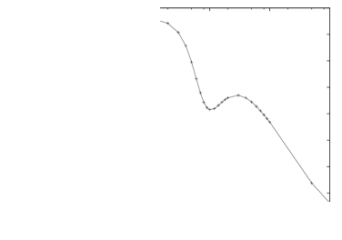
To study the effects of opacity, an average opacity from the front to the back of the data cube was used to define the detailed radiative transfer. As the opacity increases we can see from Figure 2 that the observed HI power spectra change slopes from $\sim-11/3$ to $\sim-3$.

Figure 2.: For the same model density cube this plot shows how the simulated observed HI power spectral index varies as the opacity ($\tau$) from the front to the back of the data cube is varied. This plot suggests that we may not be able to invert the observed power spectra back to the true power spectra since the function is not single-valued.

3.3. Filamentary Structures

The HI could also be confined to thin sheets or filaments. This view is supported by the images of 21cm HI emission that are being produced by the CGPS and SGPS surveys (see McClure-Griffiths 2002; and Knee 2002). Having the turbulence confined into filaments where vortices are stretched along the filament can also change the observed power spectral index. This can be realized in the model by changing $k_{x}$ to $\eta k_{x}$ where $0<\eta\leq 1$ (i.e. making the turbulence anisotropic). In Figure 3 we compare the power spectra from a an isotropic model ($\eta=1$) to a filamentary model ($\eta=0.1$). It is easily seen that filamentary structure can produce a power spectrum with a slope of $-8/3$ on the largest size scales, $l>l_{filament}^{\perp}$ where $l_{filament}^{\perp}$ is the thickness of the filament.

Figure 3.: The structure functions of models of isotropic turbulence ($\eta=1$) and turbulence in filamentary structures $(\eta=0.1$). Adding a value of two to the slope of the structure function and then multiplying by -1 gives the spectral index of the corresponding power spectrum. It is easily seen that for the filamentary case the power spectrum slope is $-8/3$ on the largest size scales.

References

Green, D.A., 1993, MNRAS, 262, 327

Dickey and Crovisier, 1983, å, 122, 282

Dickey, J.M., McClure-Griffiths, N.M., Stanimirovic, S., Gaensler, B.M. & Green, A.J., 2001, ApJ, 561, 264

Lazarian, A. & Stanimirovic, S., 2001, ApJ, 551, 53.

Lazarian, A. & Pogosyan, D., 2000, ApJ, 537, 720.

McClure-Griffiths, N.M., SGPS paper, this volume.

Knee, L., CGPS paper, this volume.