The First Detections of the Extragalactic Background Light at 3000, 5500, and 8000Å (III): Cosmological Implications

Abstract

We have used the Hubble Space Telescope Wide–Field and Planetary Camera 2, in combination with ground–based spectroscopy, to measure the integrated flux of galaxies at optical wavelengths — the extragalactic background light (EBL). We have also computed the integrated light from individual galaxy counts in the images used to measure the EBL and in the Hubble Deep Field. We find that flux in galaxies as measured by standard galaxy photometry methods has generally been underestimated by about 50%, resulting from missed flux in the outer, lower surface–brightness parts of galaxies and from associated errors in the estimated sky level. Comparing the corrected, integrated flux from individual galaxies with our total EBL measurement, we find that there is yet further light that contributes to the background that is not represented by galaxy counts, and that the total flux in individually detected sources is a factor of 2 to 3 less than the EBL from 8000 to 3000 Å. We show that a significant fraction of the EBL may come from normal galaxies at $z<4$, which are simply undetectable as a result of K-corrections and cosmological surface brightness dimming. This result is consistent with results from recent redshift surveys at $z<4$. In the context of some simple models, we discuss the constraints placed by the EBL on evolution in the luminosity density at $z>1$; while significant flux comes from galaxies beyond the current detection limits, this evolution cannot be tightly constrained by our data.

Based on our measurements of the optical EBL, combined with previously published measurements of the UV and IR EBL, we estimate that the total EBL from 0.1–1000 $\mu$m is 100$\pm$20 nW m${}^{-2}$ sr${}^{-1}$. If the total EBL were produced entirely by stellar nucleosynthesis, then we estimate that the total baryonic mass processed through stars is $\Omega_{\ast}=0.0062(\pm 0.0022)h^{-2}$ in units of the critical density. For currently favored values of the baryon density, $\Omega_{\rm B}$, this corresponds to $0.33\pm 0.12\Omega_{\rm B}$. This estimate is smaller by roughly 7% if we allow for a contribution of 7$h_{0.7}$ nW m${}^{-2}$ sr${}^{-1}$ to the total EBL from accretion onto central black holes. This estimate of $\Omega_{*}$ suggests that the universe has been enriched to a total metal mass of $0.21(\pm 0.13)Z_{\odot}\Omega_{\rm B}$, which is consistent with other observational estimates of the cumulative metal mass fraction of stars, stellar remnants, and the intracluster medium of galaxy clusters in the local universe.

1. Introduction

The integrated optical flux from all extragalactic sources is a record of the stellar nucleosynthesis in the universe and the chemical evolution which has resulted from it. In Bernstein, Freedman, & Madore 2001a (henceforth, Paper I), we presented detections of the optical EBL in the HST/WFPC2 wide-band filters F300W ($U_{300}$, $\lambda_{0}\sim$ 3000Å), F555W ($V_{555}$, $\lambda_{0}\sim$ 5500Å), and F814W ($I_{814}$, $\lambda_{0}\sim$ 8000Å) based on simultaneous data sets from Hubble Space Telescope (HST) and Las Campanas Observatory (LCO). In Bernstein, Freedman, & Madore 2001b (henceforth, Paper II), we presented details of a measurement of the diffuse foreground zodiacal light which we use in Paper I. Here we briefly summarize the results of Papers I and II and discuss the cosmological implications of these detections of the EBL.

The majority of the EBL at UV to IR wavelengths is produced by stars at restframe wavelengths of 0.1–10$\mu$m. Due to cosmic expansion, the EBL at $U_{300}$, $V_{555}$, and $I_{814}$ potentially includes redshifted light from stellar populations out to $z\sim 8$ (the redshifted Lyman–limit cut–off of the $I_{814}$ filter). Although stars themselves do not emit much light at wavelengths longer than 10$\mu$m, a complete census of the energy produced by stellar nucleosynthesis in the universe must consider the EBL over the full wavelength range 0.1-1000$\mu$m because dust in the emitting galaxies will absorb and re-radiate starlight, redistributing energy from nucleosynthesis into the thermal IR.

With 8m–class telescopes and HST, the limits of resolved–source methods (i.e., number counts, redshift surveys, QSO absorption lines, etc.) for studying star formation in the universe are being extended to ever fainter levels; however, a direct measurement of the EBL remains an invaluable complement to these methods. Galaxies with low apparent surface brightness — both intrinsically low surface brightness galaxies at low redshift and normal surface brightness galaxies at high redshift — are easily missed in surface–brightness–limited galaxy counts and consequentally in follow–up redshift surveys. Identification, not to mention photometry, of faint galaxies becomes very uncertain near the detection limits. Even efforts to understand galaxy evolution, chemical enrichment, and star formation through QSO absorption line studies appear to be biased against chemically enriched, dustier systems, as these systems can obscure QSOs which might lie behind them (Fall & Pei 1989, Pei & Fall 1995, Pettini et al. 1999). In contrast, a direct measurement of the spectral energy distribution (SED) of the EBL from the UV to the far–IR is a complete record of the energy produced by star formation and is immune to surface brightness selection effects.

In addition to energy originating from stellar nucleosynthesis, the EBL includes energy emitted by accreting black holes in quasars and active galactic nuclei. However, at optical wavelengths, the quasar luminosity functions at redshifts $z\mathrel{\hbox{\hbox to0.0pt{\hbox{\lower 4.0pt\hbox{$\sim$}}\hss}\hbox{$<$}}}5$ indicate that the optical luminosity density from quasars is a small fraction ($\sim 2.5$%) of the that from galaxies (e.g. Boyle & Terlevich 1998). In addition, our measurement of the EBL excludes any point–like sources (of which there are 3 in our images), under the prior assumption that those sources are Galactic foreground stars. We therefore expect quasars to be a negligible source of flux in our measurements of the optical EBL.

The contribution from active galactic nuclei (AGN) is more difficult to assess, as recent dynamical evidence (Richstone et al. 1998) indicates that massive black holes reside in most galaxies and sensitive optical spectroscopy (Ho et al. 1997a, 1997b) indicates that AGN have at least a weak contribution to more than 50% of nearby galaxies. Nonetheless, simple accretion models, the total X-ray background, and the X-ray to far–IR spectral energy distribution of AGN and quasars all indicate that the total contribution to the bolometric EBL from accretion onto central black holes is $\mathrel{\hbox to0.0pt{\lower 3.0pt\hbox{$\mathchar 536\relax$}\hss}\raise 2.0pt\hbox{$\mathchar 316\relax$}}15$% (see §6.2), and is emitted at thermal IR wavelengths. In principle, measurements of the EBL also constrain possible the total energy output from more exotic sources, such as gravitationally collapsing systems, brown dwarfs, and decaying particles (see Carr, Bond, & Hogan 1986, 1991 and Dwek et al. 1998 for discussions).

The outline of the paper is as follows. In §2, we give an overview of the observations and methods used to measure the EBL as discussed in Papers I and II. In §3, we summarize the individual measurements and associated errors we have obtained from each data set and the final EBL detections which result from them. In §4, we compare the measured EBL with the integrated optical flux from resolvable sources as quantified by number counts and luminosity functions. In §5, we quantify the contributions to the optical EBL which one might expected from sources which fall below the detection limits of the HDF based on explicit assumptions regarding the surface brightness, luminosity, and redshift distribution of galaxy populations in the universe. In §6, we discuss models of the SED of the EBL based on these and recent results in the far infrared. Finally, in §7 we discuss the total star formation and chemical enrichment history of the universe required to produce the bolometric flux of the EBL, and compare the inferred values to other observations of the total baryon fraction in stars and the metal mass density in the local universe. We abbreviate the adopted units ergs s${}^{-1}$ cm${}^{-2}$ sr${}^{-1}$ Å${}^{-1}$  as cgs throughout.

2. Summary of Observations

As is true of all background measurements, the difficulty in measuring the optical EBL is in differentiating it from the much brighter foregrounds: terrestrial airglow, zodiacal light (ZL), and diffuse Galactic light (DGL). Relative to the EBL flux at $\sim$5000Å, airglow and ZL are each more than 100 times brighter than the EBL. Along the most favorable lines of sight, the DGL is roughly equal in flux to the EBL. We have measured the EBL in a field which is out of the ecliptic plane and near the Galactic pole in order to optimally minimize the contributions of zodiacal light, DGL, and nearby stars (see Paper I).

In the EBL measurement presented in Paper I, we have used three simultaneous data sets to isolate the diffuse EBL from the foreground sources: (1) absolute surface photometry taken with WFPC2 aboard HST using the wide–band filters F300W ($U_{300}$), F555W ($V_{555}$), and F814W ($I_{814}$); (2) low resolution ($\sim 300$Å) surface spectrophotometry at 4000—7000Å taken with the FOS, also aboard HST; and (3) moderate resolution ($\sim$2Å) surface spectrophotometry taken with the Boller and Chivens spectrograph on the 2.5m duPont telescope at LCO. We use the two HST data sets to measure the total mean flux of the night sky, including ZL, DGL and the EBL. We avoid terrestrial airglow all together by using HST for this measurement. We then use the LCO spectra to measure the absolute surface brightness of ZL in the same field and on the same nights as the HST observations. Finally, we estimate the small DGL contribution using a scattering model which is in good agreement with the observations. We then subtract the measured ZL and the modeled DGL from the total flux measured with HST/WFPC2 through each filter and with HST/FOS. These measurements are described in detail in Papers I and II. Below, we summarize the observations, results, and accuracy of the individual measurements which contribute to the EBL detection (see Table 1).

Bright galaxies brighter are not statistically well sampled in the 4.4 arcmin${}^{2}$ WFPC2 field of view. We have, therefore, masked out any sources brighter than $V_{555}=23$AB mag in the WFPC2 images before we measured the total sky flux. To do so, we used masks which are derived from the F555W images and extend to four times the isophotal radius in those data. We use the abbreviation EBL23 as a reminder of this bright magnitude cut–off. The EBL23 detections can be combined with ground–based counts at $V_{555}\!<\!23$AB mag to obtain the total EBL. The WFPC2 surface brightness measurements have random errors of $<1$% and systematic uncertainties of 1–2% of the total background flux. From the HST/WFPC2 data alone, we can also identify a minimum flux from detectable sources. This minimum is given in Table 1, and the method used to obtain this result is summarized in §3.

The FOS spectra also provide a measurement of total flux. The random error per resolution element is around 2.1%, and the systematic uncertainty over the full range is 3.5%. The $\sim 14$ arcsec${}^{2}$ FOS field of view and $\sim 4$% systematic uncertainty make the FOS less useful than the WFPC2 for measuring the EBL. However, most of systematic uncertainty is due to the poorly constrained solid angle of the aperture and aperture correction. Both of these are wavelength–independent errors, so that the FOS spectra do provide a $\pm 1$% measurement of the color of the total background, which is dominated by zodiacal light.

The scattering which produces the ZL is well described by classical Mie theory for the large ($>10$$\mu$m), rough dust grains which populate the zodiacal dust cloud. The scattering efficiency of the dust is only weakly wavelength dependent, so that the solar spectral features are well preserved in the scattered ZL spectrum. However the broad band spectrum of the zodiacal light is redder than the solar spectrum by about 5% per 1000Å (see Paper II for further discussion) due to surface roughness of the grains, which decreases scattering efficiency at shorter wavelengths. The mean ZL flux in a narrow band can thus be measured from the apparent equivalent width of the solar Fraunhofer lines evident in its spectrum. Small color corrections can then be used to infer the full spectrum relative to that measurement. This requires moderate resolution spectra ($\sim 2$Å) with excellent flux calibration ($\pm 1$%), which can only be obtained with ground–based observations, and then only at wavelengths where atmospheric emission lines are relatively weak. We have, therefore, measured the ZL in the range 4000–5100Å using spectra taken at LCO. The resulting measurement has a statistical error of $<1$% and a systematic uncertainty of $\sim 1.2$%. This measurement has been extrapolated the 3000Å and 8000Å WFPC2 bandpasses using measurements of the color of the ZL from the FOS and ground–based LCO data.

Within the Galaxy, there is both resolved flux from discrete stars and diffuse light (diffuse Galactic light, DGL) from starlight scattered by interstellar dust. Discrete stars can simply be resolved and subtracted in the WFPC2 images. The intensity of the dust–scattered optical DGL and the 100$\mu$m thermal emission from the same dust are both proportional to the dust column density and the strength of the interstellar radiation field. To minimize the optical DGL, our field was selected to have very low 100$\mu$m emission. The remaining low–level DGL which does contribute has been estimated using a simple scattering model based on the dust column density and interstellar radiation field along the line of sight and empirical scattering characteristics for interstellar dust. The predictions of this model are in good agreement with observations of the DGL from 2500–9000Å (see Witt et al. 1997 and references therein). Finally, although isotropic line emission from warm interstellar gas is measured at all Galactic latitudes, the strongest line, H$\alpha$, does not lie within any our HST/WFPC2 bandpasses. The next strongest lines, [Oiii], are twenty times weaker and contribute negligibly to our results.

The EBL cannot be measured in typical HST data. Our HST observations were scheduled to avoid contaminating scattered light from all anticipated sources: the bright Earth limb, the Moon, and off-axis stars. Also, observations from LCO and HST were strictly simultaneous to guarantee that the ZL measured from the ground is exactly the contribution seen by HST. As an additional safeguard, observations were scheduled in 3 visits, allowing us to look for possible off–axis scattered light with the satellite oriented at different roll angles, to safeguard against unidentified photometric anomalies with the instruments, and to confirm the expected modulation in the ZL with the Earth’s orbital position.

3. Summary of EBL Detections

Table 1Summary of Measurements

Source	Bandpass	Data source	Flux	Random	Systematic
Total	F300W	hst/wfpc2	33.5	$(\pm$ 4.9%)	$[\pm$ 5.6%]
Background	F555W	hst/wfpc2	105.7	$(\pm$ 0.3%)	$[\pm$ 1.4%]
	F814W	hst/wfpc2	72.4	$(\pm$ 0.2%)	$[\pm$ 1.4%]
	F555W	hst/fos	111.5	$(\pm$ 0.7%)	$[\pm$ 2.8%]
Zodiacal	4600–4700Å	lco	109.4	$(\pm$ 0.6%)	[$\pm$ 1.1%]
Light	F300W	lco	28.5	$(\pm$ 0.6%)	[-1.1%,+1.2%]
	F555W	lco	102.2	$(\pm$ 0.6%)	[-1.1%,+1.1%]
	F814W	lco	69.4	$(\pm$ 0.6%)	[-1.3%,+1.1%]
Diffuse	F300W	dgl model	1.0	$\cdots$	[+25%,-50%]
Galactic	F555W	dgl model	0.8	$\cdots$	[+25%,-50%]
Light	F814W	dgl model	0.8	$\cdots$	[+25%,-50%]

Note. — All fluxes are in units of 1$\times 10^{-9}$ergs s${}^{-1}$ cm${}^{-2}$ sr${}^{-1}$ Å${}^{-1}$. For a source with constant flux in $F_{\lambda}$, filters F300W, F555W, and F814W have effective wavelengths $\lambda_{0}(\Delta\lambda)$ =3000(700), 5500(1200), and 8000(1500)Å. Individual sources of error contributing to each measurement are summarized in Tables 3 & 4 of Paper I and Table 1 of Paper II.

Table 2EBL Results and Uncertainties

Bandpass	Random	Systematic	Combined	EBL($\pm 1\sigma$)
	$\sigma_{R}$ (68%)	$\sigma_{S}$ (68%)	$\sigma$ (68%)
Detected EBL23 (WFPC2 + LCO)
F300W	2.1	1.5	2.5	4.0 $(\pm 2.5)$
F555W	0.6	1.3	1.4	2.7 $(\pm 1.4)$
F814W	0.4	0.9	0.0	2.2 $(\pm 1.0)$
Minimum EBL (WFPC2)
F300W	0.19	0.13	0.22	3.2 $(\pm 0.22)$
F555W	0.003	0.009	0.01	0.89 $(\pm 0.01)$
F814W	0.002	0.007	0.01	0.76 $(\pm 0.01)$
Detected EBL23 (FOS + LCO)
F555W	0.7	2.7	2.8	8.5 $(\pm 5.6)$
Flux from detected sources in HDF ($m>23$ AB mag)
F300W				0.66
F450W				0.51
F606W				0.40
F814W				0.27
Published number counts
F300W ($18<U_{300}<23$ AB mag)				0.27 $(\pm 0.05)$
F555W ($15<V_{555}<23$ AB mag)				0.49 $(\pm 0.10)$
F814W ($13<I_{814}<23$ AB mag)				0.65 $(\pm 0.13)$

Note. — All fluxes and errors are given in units of $10^{-9}$ ergs s${}^{-1}$ cm${}^{-2}$ sr${}^{-1}$ Å${}^{-1}$.

Figure 1.— Summary of EBL23 measurements, repeated from Paper I. Filled circles show the EBL23 obtained from surface photometry of the total background measured from HST/WFPC2, the zodiacal light as measured from Las Campanas Observatory, and models of the diffuse galactic light as summarized in §3. The solid, dotted, and long–dashed error bars show the combined, systematic, and random $1\sigma$ errors, respectively. The hatch–marked region shows the $1\sigma$ uncertainty in the detected EBL due to uncertainty in ZL color. The lower limit arrows connected by a dashed line indicate the total flux from individually photometered galaxies with magnitudes $23<V_{555}<30$ AB mag in the HDF catalog. The u-shaped lower limit arrows show minEBL23, which is the flux as determined by ensemble photometry from galaxies with $23<V_{555}\leq 28$ AB mag in the EBL fields.

The individual measurements which are combined to obtain our detections of the EBL are summarized in Table 1. We summarize our confidence intervals on the detected EBL23 in Table 2 and Figure 1. For comparison with the EBL23 fluxes, we have included in Table 2 the integrated flux from individually photometered sources in the HDF, as measured using the photometry package FOCAS (Jarvis & Tyson 1981, Valdes 1982) and published in Williams et al. (1996). As the values in this table show, the mean EBL23 detections in each bandpass are more than $5\times$ higher than the integrated flux in HDF galaxies as measured by standard photometry.

To help understand this large difference between the detected EBL and the flux in HDF number counts, we have measured the total flux from resolved galaxies in our WFPC2 images ($23<V_{555}<27.5$) using a method which we call “ensemble aperture photometry.” This method is uniquely suited to both our goal of a very accurate measurement of the ensemble flux of all galaxies in our images and to our data set, which has zero–point calibration accurate to $\pm 0.1\%$ over each image and negligible scattered light. This method is described in detail in Paper I and summarized below.

Briefly, we identify the total flux from detectable galaxies fainter than $V_{\rm cut}=23$ AB mag by simply masking out galaxies with $V<V_{\rm cut}$ AB mag (and all stars) and averaging the flux of every pixel in the frame. From this, we obtain the mean surface brightness of foregrounds plus all extragalactic sources, or the average surface brightness per pixel from “objects + sky.” We then mask out all detected objects using standard detection apertures (twice the isophotal area) and calculate the average flux in the remaining pixels. From this, we obtain the mean surface brightness outside of the galaxy masks, or the average surface brightness per pixel from “sky.” The difference between these two measurements is then the ensemble surface brightness of all sources within the area of the masks. This assumes that the sky level is uniform, which is the case to better than 1% accuracy in our images. By varying the bright magnitude cut–off ($V_{\rm cut}$) we choose for measuring “objects + sky,” we can isolate the flux coming from sources fainter than $V_{\rm cut}$.

As discussed in Paper I, we find that the recovered flux increases steadily with increasing mask size. For example, roughly 20% of the light from galaxies 4 magnitudes above the detection limit lies at radii $\sqrt{2}r_{\rm iso}<r<4r_{\rm iso}$ (see Figure 2), beyond the standard–size galaxy apertures ($\sqrt{2}r_{\rm iso}$) used in faint galaxy photometry packages, such as SExtractor (Bertin & Arnouts 1996) or FOCAS. Because estimates of the sky level in standard photometry packages come from just beyond the detection apertures, these sky estimates will include some fraction of the galaxies’ light and will doubly compound this error. In addition, because galaxy apertures start to significantly overlap in our images and the HDF images when they extend to $r\sim 4r_{\rm iso}$, we find that some flux from the wings of detected galaxies will inevitably contribute a pedestal level to the mean sky level in any image. We have estimated this pedestal level by Monte Carlo simulations as described in Appendix B of Paper I. The pedestal is independent of field, but does dependent on the detection limits and surface brightness characteristics of the data. For $V_{606}$ HDF images, this pedestal level is roughly 10% of the total flux from $V>23$ AB mag galaxies and, again, this error is compounded by the fact that any flux at radii beyond galaxy apertures can be include in the “sky” estimate. The true flux from $V>23$ AB mag galaxies in the HDF is therefore almost twice what is recovered by standard methods (see §4.1).

Using different values of $V_{\rm cut}$, we can quantify systematic errors in faint galaxy photometry as a function of the isophotal surface brightness limit of the data, $\mu_{\rm iso}$, and the central surface brightness of the source, $\mu_{0}$. The smaller the value of $\Delta\mu=\mu_{\rm iso}-\mu_{0}$ is for a particular galaxy, the larger the photometric error in standard aperture photometry. This problem has been discussed in the literature at length with respect to low surface brightness galaxies at low redshifts based on extrapolations of simple exponential light profiles (Disney 1976, Disney & Phillips 1983, Davies 1990); the same principle begins to apply to normal surface brightness galaxies which have low apparent surface brightness at higher redshifts due to $(1+z)^{4}$ surface brightness dimming (Dalcanton 1998).

Finally, we note that the direct measurements of the EBL23 in our data — based on surface photometry of the total integrated background, zodiacal light, and diffuse galactic light — are $2\sigma-3\sigma$ detections. However, the mean flux from detected sources is obviously an absolute minimum value for the EBL. Therefore, the strongest lower limit we can place on the flux from sources fainter than $V=23$ AB mag (EBL23) is the mean flux in detected galaxies as measured by ensemble aperture photometry in our WFPC2 data and the HDF. The strongest upper limits we can place on EBL23 are the $2\sigma$ upper limits of our direct measurements of the EBL23. In Table 2 we list (1) our direct measurements of the EBL23, and (2) the minimum values for the EBL23 (minEBL23) as identified by ensemble aperture photometry of detected sources in our WFPC2 data and the HDF. For comparison, the flux in published HDF galaxy counts and ground based counts are also listed there.

4. Comparison with Number Counts and Luminosity Functions

Whether the light originates from stellar nucleosynthesis, accretion onto compact objects, or gravitationally collapsing stellar systems, the total optical flux escaping from detected galaxies is quantified by number counts and luminosity functions. To the detection limits, number counts and luminosity functions contain exactly the same information regarding the integrated background light: the integrated flux from resolved sources is the same whether or not you know the redshift of the sources. However, in the context of predicting the EBL flux, luminosity functions contain information about the intrinsic flux distribution of the sources and thus allow us to estimate the flux from sources beyond the detection limits with better defined assumptions. In the following sections, we compare our EBL detections with the integrated flux obtained by both methods. Dust obscuration in the emitting sources will clearly reduce the UV and optical flux which escapes, but the EBL, number counts, and luminosity functions are all measurements of the escaping flux; the relative comparisons discussed in this section are therefore independent of dust extinction.

4.1. Number Counts

Figure 2.— Aperture corrections as a function of $\Delta\mu=\mu_{\rm iso}-\mu_{0}$ (isophotal minus central surface brightness) derived by “ensemble aperture photometry” of the EBL field for $V$ (thick line) and $I$ (thin line). The mean apparent magnitude in $V_{606}$ and $I_{814}$ corresponding to a particular value of $\Delta\mu$ in the HDF images is indicated by the x-axes at the top of the plot. Error bars show the $1\sigma$ statistical error in the mean corrections derived from 18 WFPC2 images of the EBL field (six exposures, three WF chips).

Figure 3.— The upper panel shows the galaxy counts as published in the HDF catalog (filled circles) with $\sqrt{N}$ error bars and the corrected number counts (open circles), as described in §4.1. The solid lines show fits to the raw number counts, which change slope slightly around $V_{606}=26$. The fit to the corrected counts is indicated by the dashed line to the detection limit and a dotted line beyond. No change in slope is apparent at the faint end for the corrected counts. All slopes are given in the text. In the lower panel, we plot the integrated flux corresponding to the galaxy counts with the same line types as in the upper panel. The data point and $1\sigma$ error bar mark the value of EBL23 (converted to $V_{606}$ from the $V_{555}$ band). The corresponding $\pm 1\sigma$ error range is emphasized by the hatch-marked region. For comparison, the lower limit arrow shows $2\sigma$ lower limit of minEBL23, the integrated flux from detected sources with $V_{606}>23$ AB mag.

Figure 4.— The same as Figure 3, but for the $I_{814}$–band. As for the $V_{606}$–band, the raw $I_{814}$ counts show a slight change in slope around 24–26 AB mag, while the corrected counts do not. All slopes are given in the text. The integrated flux of the raw and corrected counts are compared to our EBL23 $I_{814}$ detections in the lower panel, as in Figure 3.

Using “ensemble aperture photometry” to measure the total flux from galaxies as a function of magnitude in our $V_{555}$ and $I_{814}$ images of the EBL field, we find that the standard photometry methods used to produce the HDF catalog systematically underestimate the flux from each source, as summarized in §3 (see §10 and Appendix B of Paper I for a thorough discussion). We use these results to derive flux corrections as a function of $\Delta\mu=\mu_{\rm iso}-\mu_{0}$ (isophotal minus central surface brightness), which are essentially aperture corrections. These aperture corrections are similar to those found by other authors (c.f. Smail et al. 1995) and are a natural consequence of integrating an extended light profile to an insufficient radius. This effect can be quantified for exponential or de Vaucouleurs profiles, as in Dalcanton (1998). However, the corrections we show here are empirical measurements and assume nothing about the light profiles of the sources.

The corrections we derive for the two bandpasses (see Figure 2) are very similar functions of $\Delta\mu$, which indicates that the profiles of detected galaxies are not a strong function of wavelength over the baseline of observed $V$ to $I$. However, we note that a particular value of $\Delta\mu$ occurs at a brighter AB magnitude in $I_{814}$ than in $V_{606}$ because the limiting isophotal level (sky noise) in $I_{814}$ is 0.6 AB mag brighter than in $V_{606}$. The corrections are therefore larger in $I_{814}$ than they are at the same AB magnitude at $V_{606}$. The corrections in both bands include a correction which compensates for overestimates in the sky flux from foreground sources (the pedestal sky level described in §3). This correction, which accounts for errors in the local sky estimate, ranges from 0.1–0.3 mag, monatonically increasing towards fainter magnitudes. As in $V_{606}$ and $I_{814}$, aperture corrections for $U_{300}$ band will depend on the profiles of galaxies at $U_{300}$ and the surface brightness limits of the data. However, the very low signal–to–noise ratio of our F300W images prevents us from determining aperture corrections in that bandpass. The $U_{300}$ photometry is discussed further below.

We have applied the aperture corrections we derive to the individual objects in the HDF $V_{606}$ and $I_{814}$ catalogs (Williams et al.  1996), which fractionally increases the flux of each galaxy. For example, while galaxies in the HDF catalog with $V_{606}\sim 30$ AB mag have well-detected cores, less than 30% of their total flux is recovered: the total flux of a galaxy measured to have $V_{606}\sim 30$ AB mag by standard photometry methods is actually closer to $V_{606}\sim 28$ AB mag. The corrected and uncorrected (raw) galaxy counts and corresponding integrated flux with magnitude are compared in Figures 3 and 4. The integrated flux of the corrected galaxy counts roughly corresponds to the minimum value of EBL23, as the aperture corrections were derived from the calculation of the minimum EBL23 in our data. Statistical variations in galaxy counts between fields are to be expected.

The aperture corrections we apply clearly have a significant impact on the slope of faint number counts. To quantify this, we fit both the raw and corrected number counts with the usual relationship between apparent magnitude and surface number density, $N\propto 10^{\alpha m}$, where $N$ is the number of galaxies per magnitude per square degree. For the raw $V_{606}$ counts, we find that the data exhibit a change in slope around 24–26 AB mag. A single fit over the range $22<V_{606}<29.5$ AB mag gives $\alpha=0.24\pm 0.01$ with a $\chi^{2}$ per degree of freedom ($\chi^{2}/{\rm dof}$) of $1.5$. Fitting the counts brighter and fainter than 26 AB mag, respectively, we find $\alpha_{b}=0.28\pm 0.02$ with $\chi^{2}/{\rm dof}=0.9$ and $\alpha_{f}=0.21\pm 0.01$ with $\chi^{2}/{\rm dof}=1.2$ (solid lines in the upper panel of Figure 3). We ascribe this change in slope to the onset of significant photometry errors.

For the corrected $V_{606}$, counts we find that the full $22<V_{606}<27.5$ AB mag range is well fit by a slope of $\alpha=0.33\pm 0.01$ with $\chi^{2}/{\rm dof}=0.60$ (dashed line in the upper panel of Figure 3). This result suggests that photometry errors are responsible for the change in slope at the faint end of the HDF counts, and that $N(m)$ does not, in fact, significantly decline before the detection limit of the HDF at $V_{606}$. In addition, while the integrated flux in the raw galaxy counts has converged by the apparent detection limit of the HDF, the flux from the corrected galaxy counts has not (see the lower panel of Figure 3).

Figure 5.— The raw and corrected number counts from Figure 3 compared to number counts from the literature, labeled by first author. The lines indicate fits to the data using the relation $N\propto 10^{\alpha m}$; $\alpha=0.48\pm 0.1$ and $\alpha=0.33\pm 0.01$ at the bright and faint ends, respectively. Note that the slope of the corrected HDF counts is well matched to that at brighter magnitudes.

We find similar results for the $I_{814}$ counts (see Figure 4). As for $V_{606}$, the raw $I_{814}$ counts display a slight change in slope around 24–26 AB mag. We find a slope of $\alpha_{b}=0.25\pm 0.01$ with $\chi^{2}/{\rm dof}=0.6$, and $\alpha_{f}=0.19\pm 0.02$ with $\chi^{2}/{\rm dof}=2.0$, brighter and fainter than 26 AB mag, respectively. For the full range $22<I_{814}<29.5$ AB mag, we find $\alpha=0.22\pm 0.01$ with $\chi^{2}/{\rm dof}=2.1$. For the corrected $I_{814}$ counts, we find $\alpha=0.34\pm 0.01$ with $\chi^{2}/{\rm dof}=0.8$ at $22<I_{814}<27$ AB mag.

In Figure 5, we show the raw and corrected HDF counts relative to $V$- and $R$-band counts available in the literature for $V>15$ AB mag. We have converted all of the published counts to $V$-band AB mag by applying constant offsets consistent with those in Fukugita, Shimasaku, & Ichikawa (1995). These incorporate mean K–corrections based on the mean redshift corresponding to the apparent magnitude of the sample. Differences between filters will have some affect on the slope of counts in surveys which cover a large range of redshift (apparent magnitude) due to changing galaxy colors and K-corrections with increasing redshift, but these effects will average out between the multiple surveys shown. This plot shows that the aperture corrections we have applied to the HDF sources produce number counts which have a slope consistent with the slope found at brighter magnitudes.

In Figure 6, we show the same plot for the $I$–band. Again, the corrected $I_{814}$ counts display a slope which is similar to that found at magnitudes brighter than 23 AB mag. Note also that slope of the counts at $<25$ AB mag in $V$ and $I$ are the same to within the statistical errors. The aperture corrections we apply to the HDF counts at $V_{606}$ and $I_{814}$ extend this agreement to the current detection limits. The corrected counts imply that the faintest galaxies detected do not exhibit a significantly steeper slope in $V_{606}$ than in $I_{814}$, in contrast with the raw galaxy counts. This is an important constraint on galaxy evolution models.

Figure 6.— Same as Figure 5 but for the $I-$band counts. The lines indicate fits to the data using the relation $N\propto 10^{\alpha m}$; $\alpha=0.52\pm 0.1$ and $\alpha=0.34\pm 0.01$ at the bright and faint ends, respectively. Note that slope of the corrected HDF counts is well matched to the slope at brighter magnitudes, and that the slope of the $I$ and $V$ band counts are similar at all magnitudes.

Although the signal to noise in the $U_{300}$ data is too low to allow us to obtain accurate aperture corrections at that wavelength, the minimum EBL23 at $U_{300}$ implies consistent colors for faint and bright galaxies at $U-V$, as in $V-I$ (see Figure 1 and Table 2). We note, also, that the color of the integrated flux from galaxies is consistent with the color of the total background light within $2\sigma$. In other words, no exotic population of sources is required to produce the detected background.

The lack of turnover in the corrected counts strongly suggests that sources do exist at apparent magnitudes beyond the present detection limit. If we impose no limit on the apparent magnitude of sources and simply extrapolate the galaxy counts beyond $V_{606}\sim 27.5$ AB mag using $\alpha=0.33$ (dotted line in Figure 3), we obtain a prediction for the total integrated EBL23 of $1.3$$\times 10^{-9}$ cgs, which is $1\sigma$ below the measured value in the EBL field. In this case, the predicted EBL23 converges around $V_{606}\sim 50$ AB mag, which is significantly fainter than a dwarf galaxy at $z\sim 6$. However, very little flux is obtained from the faintest bins. If we impose the limit $V_{606}\sim 38$ AB mag as the faintest apparent magnitude for a realistic source (e.g., a dwarf galaxy with $M_{V}\sim-10$ AB mag at $z\sim 4$), we obtain a flux of 1.2$\times 10^{-9}$ cgs. The flux from sources with $I_{814}>23$ AB mag is $1.3$$\times 10^{-9}$ cgs if we adopt $\alpha=0.34$, with the flux converging around $I_{814}\sim 60$ AB mag. Adopting a more realistic faint cut–off of $\sim 38$ AB mag, as discussed for $V_{606}$, we obtain a total flux of $1.2$$\times 10^{-9}$ cgs, $1\sigma$ below the mean detected value of EBL23 at $I_{814}$ (see Figure 4).

In order to obtain a cumulative flux equal to the mean detected EBL (or the upper limit) from sources brighter than $\sim 38$ mag, the slope of the galaxy counts in the range 28–38 AB mag would clearly need to increase at some point beyond the current detection limit. For example, the total flux from sources $23<V_{606}<38$ AB mag will produce the mean detected EBL if the sources with $23<V_{606}<28$ AB mag obey a slope of $\alpha=0.33$ and sources with $28<V_{606}<38$ AB mag obey $\alpha=0.42$. We stress, however, that the total flux obtained from sources with such a steep faint–end slope is critically dependent on the cut of magnitude: the total flux reaches $5.1$$\times 10^{-9}$ cgs if we integrate the counts to $50$ AB mag, and to 9.0$\times 10^{-9}$ cgs if we integrate to $60$ AB mag. Recall that our $2\sigma$ upper limit on EBL23 at $V_{606}$ is $5.0$$\times 10^{-9}$ cgs. For $\alpha=0.35$ at $V>28$ AB mag, the integrated flux reaches 1.37, 1.51, and 1.57$\times 10^{-9}$ cgs (converged) for faint cut–off magnitudes of 40, 60, and 80 AB mag respectively. Although it is obviously impossible to place firm constraints on the number counts beyond the detection limit, as they may change slope at any magnitude, we conclude that it is very unlikely that the slope beyond $V_{606}\sim 28$ AB mag is steeper than $\alpha=0.42$. If the slope continues at $0.33<\alpha<0.35$, the EBL23 reaches a roughly 1.3–1.5$\times 10^{-9}$ cgs by $V_{606}\sim 40$ AB mag, $<1\sigma$ below our detected value.

Similarly, for the $I$–band the integrated flux from sources matches the mean detected EBL23 if the sources with $23<I_{814}<27$ AB mag obey a slope of $\alpha=0.34$ and sources with $27<I_{814}<39$ AB mag obey $\alpha=0.42$. For those slopes, the total flux reaches the $2\sigma$ upper limit of the EBL23 at $I_{814}$ by 50 AB mag. For $\alpha=0.36$, slightly above the slope we find for the corrected counts, the integrated flux reaches 1.31, 1.58, and 1.62$\times 10^{-9}$ cgs (converged) for faint cut–off magnitudes of 40, 60, and 80 AB mag, respectively. As for the $V$–band, we conclude that it is unlikely that the $I$–band faint–end slope is steeper than 0.42 at any magnitude. For a slope of $0.34<\alpha<0.36$ for $I>27$ AB mag, the EBL reaches 1.2–1.3$\times 10^{-9}$ by $I_{814}\sim 40$ AB mag, $1\sigma$ below our detected value.

In summary, we conclude from the corrected number counts shown in Figures 3 – 6 that sources are likely to exist beyond the detection limit of the HDF. Furthermore, if the number counts continue with the slope we measure at the faintest levels, then the predicted EBL23 is within $1\sigma$ of the detected EBL23 at both $V_{606}$ and $I_{814}$. If we extrapolate beyond the detection limits assuming the slope found from the corrected number counts, we find that less than 50% of EBL23 comes from sources beyond the current detection limit at $V_{606}$ or $I_{814}$ — the majority of the light contributing to EBL23 comes from sources which can be individually detected.

Finally, we note that our ensemble photometry method yields a statistical correction for the light lost from the wings of galaxies beyond the detection isophote. This light cannot, by definition, be recovered by standard single-object photometry. In contrast, the ensemble photometry method effectively adds together the light beyond the detection isophote from many galaxies to enable a significant measurement of that light.

4.2. Luminosity Functions

Figure 7.— The local luminosity density constructed by combining the spectral energy distributions of E/S0, Sab, and Sc galaxies weighted according to the type-dependent luminosity functions as described in §4.2 and Equation 2.

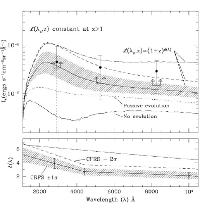
Figure 8.— The upper panel shows the spectrum of the EBL calculated by integrating the luminosity density over redshift (Equation 1) for constant luminosity density, passively evolving luminosity density, and evolution of the form ${\cal L}(\lambda,z)={\cal L}(\lambda,0)(1+z)^{\delta(\lambda)}$, with ${\cal L}(\lambda,z)$ constant at $z>1$. The lower panel shows $\delta(\lambda)$ for the three cases of $(1+z)^{\delta(\lambda)}$ as labeled in the figure and described in the text. Line types and hatch-marked regions in upper panel correspond to values of $\delta(\lambda)$ with the same line type in the lower panel. Filled circles show the mean EBL detections with $2\sigma$ error bars. The error bars are dashed where they extend below the cumulative flux in detected sources — the minimum values for the EBL — indicated by the lower limit brackets.

Figure 9.— The three panels show the spectrum of the EBL calculated assuming ${\cal L}(\lambda,z)={\cal L}(\lambda,0)(1+z)^{\delta(\lambda)}$ over the range $0<z<1.5$ (bottom panel), $0<z<2$ (middle), and $0<z<3$ (top). In all cases, the luminosity density is held constant beyond the indicated redshift limit. The hatch-marked regions each show the $\pm 1\sigma$ range of CFRS values for $\delta(\lambda)$, as in Figure 8. The integrated EBL as a function of redshift is shown in Figure 10. Luminosity density as a function of redshift is shown in Figure 11 for some combinations of $\delta(\lambda)$ and the redshift cut-off for evolution. The filled circles, error bars and lower limit symbols are as in Figure 8.

Figure 10.— The integrated EBL at $V_{555}$ contributed as a function of increasing redshift from $z=0$ to $z=10$. As marked in the figure, the lines show the integrated flux for no evolution in the luminosity density, passive evolution, and evolution of the form ${\cal L}(\lambda,z)\propto(1+z)^{\delta(\lambda)}$ for the $-1\sigma$, mean, and $+1\sigma$ range of $\delta(\lambda)$ values determined by CFRS. For each $\delta(\lambda)$, we plot the growth of the EBL with redshift if ${\cal L}(\lambda,z)$ is held constant at $z>1$, $z>1.5$, $z>2$, and $z>3$, corresponding to Figures 8 and 9.

In this section, we compare the detected EBL with the EBL predicted by luminosity functions measured as a function of redshift. To avoid unnecessary complications in defining apparent magnitude cut-offs, and to facilitate comparison with other models of the luminosity density as a function of redshift, we compare luminosity functions with the total EBL rather than with EBL23, as in the previous section. To do so, we combine the EBL23 flux measured in Paper I with the flux from number counts at brighter magnitudes, as given in Table 2. Systematic errors in photometry of the sort discussed in §4.1 are likely to be relatively small for redshift surveys because the objects selected for spectroscopic surveys are much brighter than the limits of the photometric catalogs (although see Dalcanton 1998 for discussion of the effects of small, systematic photometry errors on inferred luminosity functions). We have not tried to compensate for such effects here.

The integrated flux from galaxies at all redshifts is given by

$$I(\lambda,0)=\int_{0}^{z}{{\cal L}(\lambda_{z},z){dV_{c}(z)\over 4\pi D_{L}(z)^{2}}}$$ (1)

in which $V_{c}(z)$ is the comoving volume element, $D_{L}(z)$ is the luminosity distance, $\lambda_{0}$ is the observed wavelength, and $\lambda_{z}=\lambda_{0}(1+z)^{-1}$ is the rest–frame wavelength at the redshift of emission. To compare the detected EBL to the observed luminosity density with redshift, ${\cal L}(\lambda,z)$, we begin by constructing the SED of the local luminosity density as a linear combination of SEDs for E/S0, Sb, and Ir galaxies, weighted by their fractional contribution to the local $B$–band luminosity density:

$${\cal L}(\lambda,0)=\sum_{i}{{\cal L}_{i}(B,0){f_{i}({\lambda})\over f_{i}(B)}},$$ (2)

in which the subscript $i$ denotes the galaxy Hubble type (E/S0, Sb, or Ir), $f_{i}(\lambda)$ denotes the galaxy SED (the flux per unit rest–frame wavelength), and ${\cal L}_{i}(B,0)$ is the $B$-band, local luminosity density in ergs s${}^{-1}$ Å${}^{-1}$ Mpc${}^{-3}$. To produce the integrated spectrum of the local galaxy population, we use Hubble–type–dependent luminosity functions from Marzke et al. (1998) and SEDs for E, Sab, and Sc galaxies from Poggianti (1997). We adopt a local luminosity density of ${\cal L}_{B}=1.3\times 10^{8}hL_{\odot}$Mpc${}^{-3}$, consistent with the Loveday et al. (1992) value adopted by CFRS and also with Marzke et al. (1998). The spectrum we obtain for ${\cal L}(\lambda,0)$ is shown in Figure 7.

We note that the recent measurement of the local luminosity function by Blanton et al. (2001) indicates a factor of two higher local luminosity density than found by previous authors. Previous results are generally consistent with Loveday et al. to within 40%. Blanton et al. attribute this increase to deeper photometry which recovers more flux from the low surface brightness wings of galaxies in their sample relative to previous surveys (see discussions in §4.1), and photometry which is unbiased as a function of redshift. For the no-evolution and passive evolution models discussed below, the implications of the Blanton et al. results can be estimated by simply scaling the resulting EBL by the increase in the local luminosity density. Although the Blanton et al. results do not directly pertain to the luminosity functions measured by CFRS at redshifts $z>0.2$, they do suggest that redshift surveys at high redshifts will underestimate the luminosity density, as discussed by Dalcanton (1998).

In the upper panel of Figure 8, we compare the EBL flux we detect with EBL flux predicted by five different models for ${\cal L}({\lambda},z)$, using the local luminosity density derived in Equation 2 as a starting point. For illustrative purposes, the first model we plot shows the EBL which results if we assume no evolution in the luminosity density with redshift, i.e. ${\cal L}({\lambda},z)={\cal L}(\lambda,0)$. The number counts themselves rule out a non-evolving luminosity density, as has been discussed in the literature for over a decade; inconsistency between the detected EBL and the no-evolution model is just as pronounced. The predicted EBL for the no-evolution model is a factor of 10 fainter than the detected values (filled circles). These are $1.7\sigma$, $2.1\sigma$, and $2.2\sigma$ discrepancies at $U_{300}$, $V_{555}$ and $I_{814}$, respectively. More concretely, the no-evolution prediction is at least a factor of $12\times$, $4\times$, and $3.7\times$ lower than the flux in individually resolved sources at $U_{300}$, $V_{555}$ and $I_{814}$ (lower–limit arrows). Note that the no-evolution model still underpredicts the EBL if we rescale the local luminosity density to the Blanton et al. (2001) values. This model demonstrates the well-known fact that luminosity density is larger at higher redshifts.

The second model we plot in Figure 8 shows the effect of passive evolution on the color of the predicted EBL. In this model, we have used the Poggianti (1997) SEDs for galaxies as a function of age for $H_{0}=50$ km s${}^{-1}$ Mpc${}^{-1}$ and $q_{0}=0.225$. In the Poggianti models, stellar populations are 2.2 Gyrs old at a $z\sim 3$. The resulting ${\cal L}({\lambda},z)$ is bluer than the no-evolution model due to a combination of K-corrections and increased UV flux for younger stellar populations. The passive evolution model does provide a better qualitatively match to the SED of the resolved sources (lower limits) and EBL detections (filled circles); however, it is still a factor of $3\times$ less than the flux at $U_{300}$, and a factor of $2\times$ less than the flux we recover from resolved sources at $V_{555}$ and $I_{814}$. For the adopted local luminosity density and Poggianti models, passive evolution is therefore not sufficient to produce the detected EBL. Again, the passive evolution adopted here still underpredicts the EBL if we rescale the local luminosity density by a factor of two to agree with the Blanton et al. (2001) value.

As a fiducial model of evolving luminosity density, we adopt the form of evolution implied by the CFRS redshift survey (Lilly et al. 1996, hereafter CFRS) and Lyman-limit surveys of Steidel et al. (1999): ${\cal L}({\lambda},z)={\cal L}(\lambda,0)(1+z)^{\delta(\lambda)}$ over the range $0<z<1$ and roughly constant luminosity density at $1<z<4$. The remaining three models shown in Figure 8 test the strength of evolution of that form which is allowed by the EBL detections. The hatch-marked region shows the EBL predicted for values of $\delta(\lambda)$ which represent the $\pm 1\sigma$ range found by CFRS for the redshift range $0<z<1$. The value of the exponent $\delta(\lambda)$ is indicated in the lower panel of Figure 8, and the hatch–marked region reflects the uncertainty in the high redshift luminosity density due to the poorly constrained faint–end slope of the luminosity functions. This $\pm 1\sigma$ range of the predicted EBL is consistent with the detected EBL at $U_{300}$, but is inconsistent with the EBL detections at $V_{555}$ and $I_{814}$ at the $1\sigma$ level of both model and detections. It is, however, consistent with the integrated flux in detected sources at $V_{555}$ and $I_{814}$.

To test the range of evolution allowed by the full $\pm 2\sigma$ range of the EBL detections, we can explore two possibilities: (1) stronger evolution at $0<z<1$, shown in Figure 8; and (2) evolution continuing beyond $z=1$, shown in Figures 9, 10, and 11. Addressing the possibility of constant luminosity density at $z>1$, the dashed line in the upper panel of Figure 8 shows the EBL predicted by the $2\sigma$ upper limit for $\delta(\lambda)$ from CFRS; the dot–dashed line corresponds to the value of $\delta(\lambda)$ required to obtain the upper limits of the EBL detections at all wavelengths. Note that the latter implies a value for ${\cal L}(4400\AA,1)$ which is $\sim 10\times$ higher than the value estimated by CFRS. This result emphasizes that the $2\sigma$ interval of the EBL detections span a factor of $4$ in flux at 4400Å, and thus the allowed range in the luminosity density for $\lambda<4400$Å and $0<z<1$ is similarly large. Also, for each model in which the luminosity density is constant at $z>1$, less than $50$% of the EBL will come from beyond $z=1$ due to the combined effects of K-corrections and the decreasing volume element with increasing redshift (see Figure 10).

Figure 11.— The luminosity density at $U_{300}$ as a function of redshift corresponding to limiting cases plotted in Figure 9. The hatch–marked region indicates the $\pm 1\sigma$ range given by the CFRS measurements of $\delta(\lambda)$ over the range $0<z<1$. The horizontal line segments show the luminosity density corresponding to the $-1\sigma$ limit for $\delta(\lambda)$ held constant at $z>1.5$; the mean value for $\delta(\lambda)$ held constant at $z>2$; and the $+1\sigma$ limit for $\delta(\lambda)$ held constant at $z>3$.

Evolution continuing beyond $z=1$ is possible if the Lyman–limit-selected surveys have not identified all of the star formation at high redshifts, and estimates of the luminosity density at $3\mathrel{\hbox to0.0pt{\lower 3.0pt\hbox{$\mathchar 536\relax$}\hss}\raise 2.0pt\hbox{$\mathchar 316\relax$}}z\mathrel{\hbox to0.0pt{\lower 3.0pt\hbox{$\mathchar 536\relax$}\hss}\raise 2.0pt\hbox{$\mathchar 316\relax$}}4$ are subsequently low. Figures 9 and 10 show the EBL predicted by models in which the luminosity density increases as $(1+z)^{\delta(\lambda)}$ to redshifts of $z=1.5$, 2 and 3. Clearly, significant flux can come from $z>1$ if the luminosity density continues to increase as a power law. The rest–frame $U_{300}$ luminosity density is plotted as a function of redshift in Figure 11 for limiting values of the cut–off redshift for evolution and $\delta(\lambda)$. Although the strongest evolution plotted over–predicts the detected EBL, our detections are clearly consistent with some of the intermediate values of the $\delta(\lambda)$ and increasing luminosity density beyond $z=1$. For example, the mean rate of increase in the luminosity density found by CFRS can continue to redshifts of roughly 2.5–3 without over-predicting the EBL.

In all models, we have adopted the same cosmology ($h=0.5$ and $\Omega=1.0$) as assumed by CFRS and Steidel et al. (1999) in calculating ${\cal L}(\lambda,z)$ and $\delta(\lambda)$. Although the luminosity density inferred from these redshift surveys depends on the adopted cosmological model, the flux per redshift interval is a directly observed quantity. The EBL is therefore a directly observed quantity over the redshift range of the surveys, and is also model–independent. To the degree that the luminosity density becomes unconstrained by observations at higher redshifts, the EBL does depend on the assumed (not measured) luminosity density and on the adopted cosmology through the volume integral. Although dependence of the predicted EBL on $H_{0}$ cancels out between the luminosity density, volume element, and distance in Equation 1, $H_{0}$ has some impact through cosmology–dependent time scales, which affect the evolution of stellar populations. If the luminosity density is assumed to be constant for $z>1$, the predicted EBL increases by 25% at $V_{555}$ for ($\Omega_{M}=0.2,\Omega_{\Lambda}=0$) and corresponding values of $\delta(\lambda)$, and decreases by 50% for (0.2,0.8). The luminosity densities corresponding to the $2\sigma$ upper limit of the detected EBL change by the same fractions for the different cosmologies if $\cal L$ is constant at $z>1$. Similarly, for models in which the luminosity density continues to grow at $z>1$, the luminosity density required to produce the EBL will be smaller if we adopt (0.2,0) than (1,0), and smaller still for (0.2,0.8). The exact ratios depend on rate of increase in the luminosity density.

Several authors (Treyer et al. 1998, Cowie et al. 1999, and Sullivan et al. 2000) have found that the $\cal L$ at UV wavelengths (2000-2500Å) is higher than claimed by CFRS (2800Å) in the range $0<z<0.5$ and have found weaker evolution in the UV luminosity density, corresponding to $\delta(2000\AA)\sim 1.7$. The implications for the predicted EBL can be estimated from the plots of the ${\cal L}(U_{300},z)$ shown in Figure 11, and the corresponding EBL in Figures 9 and 10. For instance, if the local UV luminosity density is a factor of 5 higher than the value we have adopted and if $\delta(2000\AA)\sim 1.7$ over the range $0<z<1$, then the rest–frame UV luminosity density at $z=1$ is similar to that measured by CFRS, and the predicted $U_{300}$ EBL will be roughly 3.5$\times 10^{-9}$ cgs, very similar to the EBL we derive from our modeled local luminosity density and the mean values for $\delta(\lambda)$ from CFRS.

4.3. Discussion

Evolution in the luminosity density of the form $(1+z)^{\delta(\lambda)}$ at $0<z<1$ and slower growth or stabilization at $z>1$, such as suggested by redshift surveys at $0<z<4$, is consistent with the detected EBL for values of $\delta(\lambda)$ consistent with CFRS. The strongest constraints we can place on the EBL span a factor of 5 in flux. As such, stronger evolution between $0<z<1$ than reported by CFRS or continuing evolution at $z>1$ cannot be tightly constrained. We note that recent results from Wright (2000), which constrain the 1.25$\mu$m EBL flux to be 2.1($\pm 1.1$)$\times 10^{-9}$ cgs, are in good agreement with our results, but do not improve the constraints on the high redshift optical luminosity density over those discussed above.

In contrast with our results, previous authors have claimed good agreement between the flux in the raw number counts from the HDF and integrated flux in the measured CFRS luminosity density to $z=1$ under the assumption that the luminosity density drops rapidly at $z>1$ (Madau, Pozzetti, & Dickinson 1998, Pozzetti et al. 1998). In that work, the errors in faint galaxy photometry which cause $\sim 50$% underestimates of the total light from $V>23$ galaxies (discussed in §4.1) are compensated by the assumption that the luminosity density drops rapidly beyond $z=1$. That assumption was based on measurements of the flux from Lyman–limit systems in the HDF field by Madau et al (1996), which are substantially lower than measurements by Steidel et al. (1999) due to underestimates of the volume corrections and to the small–area sampling. We find that the detected EBL is not consistent with luminosity evolution comparable to the CFRS measured values at $0<z<1$ if the luminosity density drops rapidly at $z>1$.

5. Flux from Sources Below the Surface Brightness Detection Limit

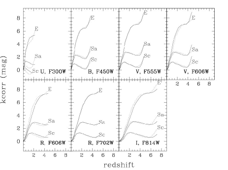
Figure 12.— K-corrections for various filters as a function of redshift calculated using Poggianti (1997) SEDs for present day E, Sa, and Sc galaxies. Bandpasses are standard Johnson/Cousins filters and the corresponding WFPC2 filters, shown with solid and dotted lines, respectively.

The fractional EBL23 flux which comes from detected sources is simply the ratio of the flux in detected sources (measured by “ensemble photometry”) to the detected EBL23 ($\pm 2\sigma$ limits). The maximum fractional EBL23 flux coming from undetected sources is what remains: 0-65% at $U_{300}$, 0-80% at $V_{555}$, and 0-80% at $I_{814}$. Although these limits include the possibility of no additional contribution from undetected sources, it is worthwhile to note that if the progenitor of a normal disk galaxy at $z=0.1$ (central surface brightness $\mu_{0}(V)\sim 21.3$ mag arcsec${}^{-2}$ and $V\sim 22$ mag) existed at $z\sim 2$, then the $z\sim 2$ progenitor would have a core surface brightness (within $0.2\times 0.2$ arcsec${}^{2}$) of $\sim 26$ mag arcsec${}^{-2}$ for standard K–corrections and passively evolving stellar populations (e.g. Poggianti 1997), which is roughly the detection limit for the HDF. In particular, regardless of the exact evolutionary or k–corrections, dimming due to cosmological effects alone (redshift and angular resolution) produce $\sim 5$ mag of surface brightness dimming. This effect is independent of wavelength, so that dimming at other bandpasses is similar, modulo differences in the evolutionary and K–corrections (shown in Figures 12, 13 and 14). At $I$, for example, the drop in surface brightness for a disk galaxy at $z\sim 2$ relative to $z\sim 0$ is $\sim 0.5$ mag greater than for $V$. The progenitor of a typical disk galaxy at $z=0.1$, which has $V-I\sim 0.9$ and $\mu_{0}(I)\sim 20.3$ mag arcsec${}^{-2}$ (de Jong & Lacey 2000), will have $V-I\sim 0.5$ at $z\sim 2$ and $\mu_{0}(I)\sim 25.5$. Thus the typical disk galaxy at $z\sim 2$ is close to the HDF detection limit in $I$ as well as $V$. Irrespective of the color evolution with redshift, the point is that cosmological surface brightness dimming alone suggests that a significant fraction of the EBL23 may come from normal galaxies at redshifts $z<4$ which are undetectable in the HDF. Furthermore, recent redshift surveys for low surface brightness (LSB) galaxies now suggest that the distribution of galaxies in $\mu_{0}$ is nearly flat for $\mu_{0}>22.0B$ mag arcsec${}^{-2}$ at some luminosities (Sprayberry et al. 1997, Dalcanton et al. 1997, O’Neil & Bothun 2000, Blanton et al. 2001, Cross et al. 2001). If such populations exist at high redshift, they may contribute significant flux to the EBL as presently undetectable sources.

In this section, we explore the possible contributions to the EBL23 from galaxies at all redshifts which escape detection in the HDF because of low apparent surface brightness. To do so, we have simulated galaxy populations at redshifts $0<z<10$ as the passively evolving counterparts of local galaxy populations and then “observed” the simulated galaxies through the Gaussian $0.1^{\prime\prime}$ FWHM point spread function of WFPC2. We define the surface brightness detection threshold to be consistent with the $5\sigma$ detection limits of the HDF images (see Table 3), which correspond to roughly the turn–over magnitude in the number counts. This exercise is not meant to approximate realistic galaxy populations at high redshift; the evolution of galaxy populations in surface brightness, luminosity, and number density is so poorly constrained at present that more specific modeling is unwarranted. The models discussed here simply address the question: how much of the total flux from a local-type galaxy population at a redshift $z$ can be resolved into individual sources?

5.1. Models

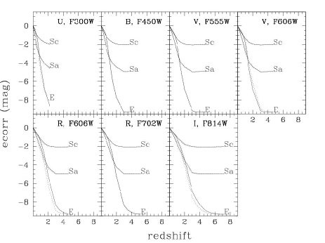
Figure 13.— Evolutionary corrections for various filters as a function of redshift calculated using Poggianti (1997) SEDs for E, Sa, and Sc galaxies evolving passively with redshift. Bandpasses are standard Johnson/Cousins filters and the corresponding WFPC2 filters, shown with solid and dotted lines, respectively.

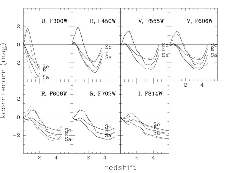
Figure 14.— The sum of the evolutionary and K–corrections for Johnson/Cousins (solid lines) and WFPC2 filters (dotted lines) shown in Figures 12 and 13.

Figure 15.— The dark hatched regions in the three panels show the surface brightness distribution as a function of luminosity for the models adopted here (Model A, Model B, and PE). For comparison, the light hatched region shows the surface brightness distribution as a function of luminosity (relative to $L^{*}$) as found by Blanton et al. (2001).

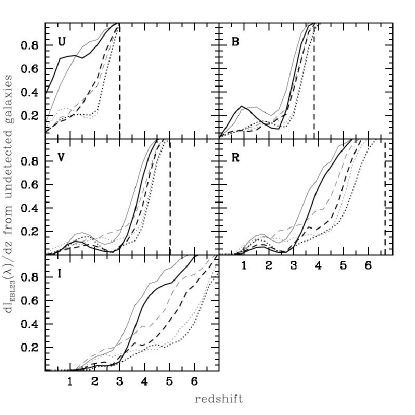
Figure 16.— For the Johnson/Cousins bandpasses indicated in each panel, we plot the EBL from galaxies which are not individually detected in each redshift bin, normalized by the total EBL in each redshift bin. Models A, B and PE are marked with solid, dashed, and dotted lines, respectively. Thick lines correspond to simulations run with $h=0.7$, $\Omega_{0}=1.0$, while thin lines correspond to $h=0.7$, $\Omega_{0}=0.2$. The dotted vertical line in each panel indicates the Lyman limit for the band-pass.

We have considered three models for the central surface brightness distributions of disk galaxies in order to explore the possible contributions from LSB galaxies. These models are taken from Ferguson & McGaugh 1995 (FM95) and can be generally described as follows: a standard passive evolution model in which all galaxies have central surface brightnesses in the range $21<\mu_{0}(B_{J})<22$ mag arcsec${}^{-2}$ (Model PE); an LSB–rich model (Model A), in which galaxies of all luminosities have $21.5<\mu_{0}(B_{J})<25$ mag arcsec${}^{-2}$; and a more conservative LSB model (Model B), in which $\mu_{0}$ is monotonically decreasing for galaxies fainter than $L/L^{\ast}<1$ and $21<\mu_{0}(B_{J})<22$ mag arcsec${}^{-2}$ otherwise (see Figure 15). We include passive luminosity evolution in all three models, as the no–evolution models have been clearly ruled out by both number counts and our own EBL results. As Model A (Model PE) has a broader (narrower) surface brightness distribution than is found by recent LSB surveys (Sprayberry et al. 1997, Dalcanton et al. 1997, O’Neil & Bothun 2000), these models are taken as illustrative limits on the fraction of low surface brightness galaxies in the local universe. Recent determinations of the number density of galaxies as a function of both luminosity and surface brightness (c.f. Blanton et al. 2001 and Cross et al. 2001) are well bracketed by these models: Model A allows for too many low surface brightness galaxies, while the PE model clearly allows for too few (see Figure 15).

As described in Table 2 of FM95, each surface brightness distribution model has been paired with a tuned luminosity function, so that each model matches the observed morphological distributions and luminosity functions recovered by local redshift surveys. The models include identical distributions in the relative number of galaxies of different Hubble types (E/S0, S0, Sab, Sbc, and Sdm), which are described by bulge-to-disk flux ratios of 1.0, 0.4, 0.3, 0.15, and 0.0, with small scatter. The bulge components for all galaxies have E-type SEDs, and S0 to Sdm galaxies have disk components with E, Sa, Sb, and Sc-type SEDs, for which we have used the Poggianti (1997) models. Bulges were given r${}^{1/4}$–law light profiles with central surface brightnesses drawn from the empirical relationship found by Sandage & Perelmuter (1990), $\mu_{0}=-0.48M_{B_{T}}+11.02$. For disk components, we adopted exponential light profiles, with surface brightnesses drawn from the 3 model distributions for disk galaxies listed above.

We have calculated passive evolution and K–corrections from the population synthesis models and SEDs of Poggianti (1997), shown in Figures 12 and 13, and we have assumed uniform comoving density as a function of redshift in all cases. All models were run with $H_{0}=50$ and 70 km s${}^{-1}$ Mpc${}^{-1}$ and ($\Omega_{M}=0.2,\Omega_{\Lambda}=0$), (1,0), and (0.2, 0.8). Different values of $H_{0}$ have little effect ($<10$%) on the integrated counts or background. The total background increases for models with larger volume — (1,0), (0.2,0), and (0.2,0.8), in order of increasing volume — but the fractional flux as a function of redshift changes by less than 10% with cosmological model.

All three models under-predict the number counts and integrated flux in observed sources, as expected, and will clearly under-predict the total EBL as illustrated in the passive evolution model discussed in §4.2.

5.2. Results

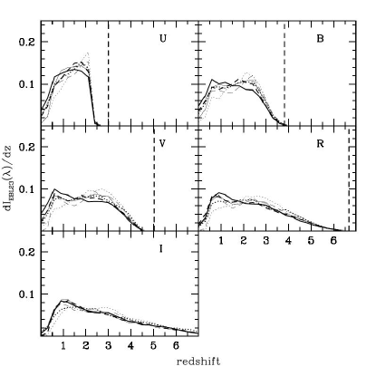
Figure 17.— For the Johnson/Cousins bandpasses indicated in each panel and the models discussed in the text, we plot the redshift distribution of the EBL — the differential EBL from all galaxies as a function of redshift, normalized by the total EBL in each band. Line types correspond to the models as described in the caption of Figure 16. In this plot, cosmological models are virtually indistinguishable because the fractional volume per redshift bin changes very little with $\Omega$. The dashed vertical line in each plot indicates the redshift corresponding to the Lyman limit for the central wavelength of each bandpass.

Figure 18.— The lines show the fraction of the EBL that comes from undetected galaxies as predicted by our models. Line types are as in Figure 16. Arrows show the upper limits on the fraction of the EBL which might come from undetected galaxies based on the EBL detections summarized in §3 and Table 2. These arrows show the ratio of flux recovered by ensemble photometry (from resolved galaxies) and the two sigma upper limits of our EBL detection. See §5.2 for discussion.

In Figures 16 through 18, we plot the distribution of the total flux from the modeled galaxy populations as a function of redshift, wavelength, and origin (detectable or undetectable galaxies). Detection limits applied at each bandpass are the $5\sigma$ detection limits of the HDF catalog (Williams et al. 1996), with appropriate conversions to the ground–based filter bandpasses, summarized in Table 3. The conversions given in this Table include differences in the evolutionary corrections and K-corrections between WFPC2 and UBVRI filters (see Figures 12–14), which are generally less than 0.3 mag and change by less than 0.1 mag at $z\mathrel{\hbox to0.0pt{\lower 3.0pt\hbox{$\mathchar 536\relax$}\hss}\raise 2.0pt\hbox{$\mathchar 318\relax$}}0.5$. We only consider sources with $V>23$ mag here, and we assume perfect photometry for sources which meet the detection criteria.

Table 3Adopted Detection Limits of the HDF

HST	$\mu_{\rm core}$	$m$	Johnson/Cousins	$\mu_{\rm core}$	$m$
Filter	AB mag arcsec${}^{-}2$	AB mag	Filter	mag arcsec${}^{-}2$	mag
wfpc2/F300W	25.0	27.5	U	23.9	26.4
wfpc2/F450W	25.8	28.3	B	25.8	28.3
wfpc2/F606W	26.3	28.8	V	25.9	28.4
wfpc2/F606W	26.3	28.8	R	25.5	28.0
wfpc2/F814W	25.8	28.3	I	25.2	27.7

In Figure 16, we show the fraction of the total flux which comes from undetected sources as a function of redshift. For all models, this plot demonstrates that if galaxy populations at higher redshifts are the passively evolving counterparts of those in the local universe, the flux from undetected sources becomes significant by redshifts of $1<z<3$. The undetected fraction is the highest in the $U$ band, due to the high sky noise and low sensitivity of the F300W HDF images relative to the other bandpasses which define our detection criteria. The detection fractions are similar in $B$ and $V$, where detection limits and galaxy colors are similar. The fraction of light from undetected sources in $I$ is small at $z<2$ due to the generally red color of galaxies, but increases beyond that redshift due to cosmological effects. Model A, with the largest fraction of low $\mu_{0}$ galaxies, has the sharpest increase in the undetected EBL with redshift, as expected. A balance between evolutionary– and K–corrections at $1<z<3$ slow this trend and cause the dip in the fraction of undetected light in $B$, $V$, and $R$. The Lyman limit for each band obviously represents the highest redshift from which one could expect to detect flux.

In Figure 17, we plot the distribution of light with redshift in these models. All three models have roughly the same distribution of $I_{\rm EBL}(\lambda,z)$ simply because all models employ a uniform comoving number density with redshift and the same passive luminosity evolution. Although we do not intend to realistically predict the redshift distribution of the EBL, we show this plot for comparison with Figure 16 to indicate the redshifts at which the majority of undetected galaxies lie in these models. Looking at Figures 16 and 17 together, it is clear that while $40-100$% of the $B$–band flux from $z>3$ is in undetectable sources for all of the models considered, only a small fraction of the total $B$–band EBL comes from those redshifts. Thus, the majority of the light from unresolved sources comes from $1<z<3$ at $B$ for local-type galaxy populations in this scenario.

Figure 18 shows the fraction of EBL23 coming from undetected sources as a function of wavelength. These models indicate that 10–35% of the light from the high redshift counterparts of local galaxy populations would come from (individually) undetected sources in bandpasses between $V$ and $I$ with sensitivity limits similar to the HDF, 15–40% would come from undetected sources at $B$, and 20–70% would come from undetected sources at $U$. This trend with wavelength (smallest fraction of undetected sources around 5000Å) follows the trend in the detection limits of the HDF bandpasses, as discussed in §4.1. Note that the color of the EBL23 is similar to the color of detected galaxies (see Figure 1) in $V$ and $I$, as is the $2\sigma$ lower limit of minEBL23 (see also Table 2).

We stress again that cosmological surface brightness dimming and the fraction of LSBs in each model are the dominant effects which govern how much light comes from undetected sources and these effects are independent of wavelength. The passive luminosity evolution corrections, K–corrections, and the HDF-specific detection limits we adopt will determine how the fraction of undetected sources varies with wavelength. Finally, we note that although the surface brightness distribution of galaxies as a function of redshift is presently unconstrained, and may or may not show significant variation with redshift, it is unlikely that the surface brightness distribution at any redshift is significantly more extreme than the distribution bracketed by our models. Bearing these uncertainties in mind, we can use the results of these models to estimate the value of EBL23 based on the minEBL23 (the flux in individually detected galaxies from ensemble aperture photometry) and the undetected fractions summarized above. If the universe is populated by galaxies with surface brightness distributions like those in the local universe, then these models suggest the following values for EBL23: 2.6–7.0$\times 10^{-9}$ cgs, 1.0–1.3$\times 10^{-9}$ cgs, and 0.9–1.2$\times 10^{-9}$ cgs at $U_{300}$, $V_{555}$ and $I_{814}$, respectively. These ranges are in good agreement with our detected values for EBL23 (see Table 2), and with the estimates of the EBL23 based on the corrected number counts we presented in §4.1.

6. The Bolometric EBL (0.1–1000$\mu$m)

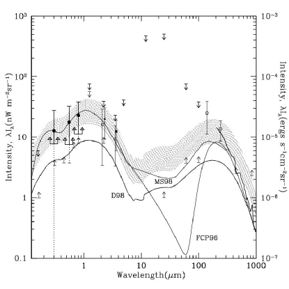
Figure 19.— EBL detections, limits, and models as a function of wavelength. The filed circles show the EBL detections with $2\sigma$ error bars and lower limit symbols as defined in Figure 8. Also plotted are lower limits from Armand et al. (1994) at 2000Å, the HDF (Williams et al. 1996), Gardner et al. (1997) at 2.2$\mu$m, IRAS (Hacking & Soifer 1991) at 10–100$\mu$m, and Blain et al. (1999) at 450 and 850 $\mu$m. These lower limits are based on the integrated flux in detected sources at each wavelength. Upper limits marked in bold are from Hurwitz, Bowyer, & Martin (1991) at 1600Å and DIRBE (Hauser et al. 1998). The open circles indicate DIRBE detections. The bold line at 125–1000$\mu$m shows the FIRAS detection (Fixsen et al. 1998). Detections in the near–IR are from Wright (2000, filled triangle), Gorjian, Wright, & Chary (2000, open squares), and Wright & Reese (2000, filled square). The lines which indicate models are all labeled and are from Malkan & Stecker (1998, MS98), Dwek et al. (1998, D98), and Fall, Charlot, & Pei (1996, FCP96) as described in §6. The shaded region shows the D98 model rescaled to match the range allowed by our EBL detections.

In Figure 19, we plot EBL detections to date, together with the integrated light in detectable sources (lower limits to the EBL) in units of $\nu I_{\nu}$ between 0.1 and 1000$\mu$m. The DIRBE and FIRAS detections at $\lambda>100$$\mu$m and the lower limit from IRAS detected galaxies at 10-100$\mu$m  indicate that energy is contained in the far infrared portion of the spectrum. Given that light from stellar nucleosynthesis is emitted at wavelengths $0.1-10$$\mu$m, Figure 19 emphasizes the fact that 30% or more of the light from stellar nucleosynthesis has been redistributed into the wavelength range $10-1000$$\mu$m by dust absorption and re-radiation and, to a lesser degree, by cosmological redshifting. Realistic estimates of the total energy from stellar nucleosynthesis must therefore be based on the bolometric EBL from the UV to IR. In lieu of accurate measurements in the mid–IR range, realistic models of dust obscuration and the dust re–emission spectrum (dust temperature) are needed. To discuss the optical EBL in the context of star formation, we must therefore first estimate the bolometric EBL based on the optical EBL detections presented here and current measurements in the far-IR. We do so in the following section.

6.1. Models

Efforts to predict the intensity and spectrum of the EBL by Partridge & Peebles (1967) and Harwit (1970) began with the intent of constraining cosmology and galaxy evolution. Tinsley (1977, 1978) developed the first detailed models of the EBL explicitly incorporating stellar initial mass functions (IMFs), star formation efficiencies, and stellar evolution. Most subsequent models of the EBL have focused on integrated galaxy luminosity functions with redshift–dependent parameterization, with particular attention paid to dwarf and low surface brightness galaxies (see discussions in Guiderdoni & Rocca-Volmerange 1990, Yoshii & Takahara 1988, and Väisänen 1996).

More recent efforts have focused on painting a detailed picture of star formation history and chemical enrichment based on the evolution of resolved sources. The evolution of the UV luminosity density can be measured directly from galaxy redshift surveys (e.g., Lilly et al. 1996, Treyer et al. 1998, Cowie et al. 1999, Steidel et al. 1999, Sullivan et al. 2000), from which the star formation rate with redshift, $\dot{\rho}_{\ast}(z)$, can be inferred for an assumed stellar IMF. The mean properties of QSO absorption systems with redshift can also be used to infer $\dot{\rho}_{\ast}(z)$, either based on the decrease in Hi column density with decreasing redshift (under the assumption that the disappearing Hi is being converted into stars) or based on the evolution in metal abundance for an assumed IMF and corresponding metal yield (e.g., Pettini et al. 1994; Lanzetta, Wolfe, & Turnsheck 1995; Pei & Fall 1995). Estimates of the star formation rate at high redshift have also come from estimates of the flux required to produce the proximity effect around quasars (e.g., Gunn & Peterson 1965, Tinsley 1972, Miralda-Escude & Ostriker 1990). Using these constraints, the full spectrum of the EBL can then be predicted from the integrated flux of the stellar populations over time.

Unfortunately, all methods for estimating $\dot{\rho}_{\ast}(z)$ contain significant uncertainties. The star formation rate deduced from the rest-frame UV luminosity density is very sensitive to the fraction of high mass stars in the stellar initial mass function (IMF) and can vary by factors of 2-3 depending on the value chosen for the low mass cut off (see Leitherer 1999, Meader 1992). Aside from the large uncertainties in the measured UV luminosity density due to incompleteness, resolved sources at high redshift are biased towards objects with dense star formation and may therefore paint an incomplete picture of the high-$z$ universe. Also, large corrections for extinction due to dust must be applied to convert an observed UV luminosity density into a star formation rate (Calzetti 1997).

The SFR inferred from QSO absorption systems, whether from consumption of Hi or increasing metal abundance, is also subject to a number of uncertainties. In all cases, samples may be biased against the systems with the most star formation, dust, and metals: dusty foreground absorbers will obscure background QSOs, making the foreground systems more difficult to study. In addition, large scale outflows, a common feature of low–redshift starburst galaxies, have recently been identified in the high–redshift rapidly star–forming Lyman break galaxies (Pettini et al. 2000), suggesting that changes in the apparent gas and metal content of such systems with redshift may not have a simple relationship to $\dot{\rho}_{\ast}(z)$ and the metal production rate. The mass loss rate in one such galaxy appears to be as large as the star formation rate, and the recent evidence for Civ in Ly-$\alpha$ forest systems with very low Hi column densities ($\mathrel{\hbox{\hbox to0.0pt{\hbox{\lower 4.0pt\hbox{$\sim$}}\hss}\hbox{$<$}}}$$\times 10^{14}$ cm${}^{-2}$) suggests that dilution of metals over large volumes may cause underestimates in the apparent star formation rate derived from absorption line studies (see Ellison et al. 1999, Pagel 1999, Pettini 1999 and references therein).

Finally, regarding the predicted spectrum of the EBL, the efforts of Fall, Charlot, & Pei (1996) and Pei, Fall, & Hauser (1998) emphasize the need for a realistic distribution of dust temperatures in order to obtain a realistic near-IR spectrum.

With these considerations in mind, we have adopted an empirically motivated model of the spectral shape of the EBL from Dwek et al. (1998, D98). This model is based on $\dot{\rho}_{\ast}(z)$ as deduced from UV–optical redshift surveys and includes explicit corrections for dust extinction and re–radiation based on empirical estimates of extinction and dust temperature distributions at $z=0$. The comoving luminosity density can then be expressed explicitly as the sum of the unattenuated stellar emission, $\epsilon_{s}(\nu,z)$, and the dust emission per unit comoving volume, $\epsilon_{d}(\nu,z)$. Equation 1 then becomes

$$I(\lambda,0)=\int_{0}^{z}{[\epsilon_{s}(\nu,z)+\epsilon_{d}(\nu,z)]dV_{c}(z)\over 4\pi D_{L}(z)^{2}}\quad.$$ (3)

D98 estimate the ratio $\epsilon_{d}(\lambda,0)/\epsilon_{s}(\lambda,0)$ by comparing the UV–optical luminosity functions of optically detected galaxies with IR luminosity function of IRAS selected sources. Using values of ${\cal L}=(1.30\pm 0.7)\times 10^{8}L_{\odot}$ Mpc${}^{-3}$ for the local stellar luminosity density at 0.1–10$\mu$m and ${\cal L}=0.53\times 10^{8}L_{\odot}$ Mpc${}^{-3}$ for the integrated luminosity density of IRAS sources, Dwek et al. obtain $\epsilon_{d}(\lambda,0)$/$\epsilon_{s}(\lambda,0)\sim 0.3$. The redshift independent dust opacity is assumed to be an average Galactic interstellar extinction law normalized at the $V$–band to match this observed extinction. D98 then calculate the EBL spectrum using the UV-optical observed $\dot{\rho}_{\ast}(z)$, a Salpeter IMF ($0.1<M<120M_{\odot}$), stellar evolutionary tracks from Bressan et al. (1993), Kurucz stellar atmosphere models for solar metallicity, redshift–independent dust extinction, and dust re-emission matching the SED of IRAS galaxies.

The starting-point UV-optical $\dot{\rho}_{\ast}(z)$ for this model is taken from Madau, Pozzetti, & Dickinson (1998), which under-predicts the detected optical EBL presented in Paper I (see §4.3). While D98 discuss two models which include additional star formation at $z\mathrel{\hbox{\hbox to0.0pt{\hbox{\lower 4.0pt\hbox{$\sim$}}\hss}\hbox{$>$}}}1$, the additional mass is all in the form of massive stars which radiate instantaneously and are entirely dust-obscured, resulting in an ad hoc boost to the far IR-EBL. We instead simply scale the initial Dwek et al. model by $\times 2.2$ to match the $2\sigma$ lower limit of our EBL detections and $\times 4.7$ to match the $2\sigma$ upper limit, in order to preserve the consistency of the D98 model with the observed spectral energy density at $z=0$. In that any emission from $z>1$ will have a redder spectrum than the mean EBL, simply scaling in this way will produce a spectrum which is too blue. However, as discussed in §4.2, it is also possible that the $z<0.5$ UV luminosity density has been underestimated by optical surveys, so that the bluer spectrum we have adopted may be appropriate. Note that the resulting model is in excellent agreement with recent near-IR results at 2.2 and 3.5$\mu$m (Wright & Reese 2000; Gorjian, Wright, & Chary 2000; Wright 2000) and also with the DIRBE and FIRAS results in the far-IR. Adopting this model, we estimate that the total bolometric EBL is $100\pm 20$ nW m${}^{-2}$sr${}^{-1}$, where errors are $1\sigma$ errors associated with the fit of that template to the data.

Due to the corrections which account for the redistribution by dust of energy into the IR portion of the EBL, the star formation rate implied by the unscaled (or scaled) D98 model is 1.5 (or 3.3–7.1) times larger than the star formation rate adopted by Madau et al. (1998). The dust corrections used by Steidel et al. (1999) produce a star formation rate which is roughly 3 times larger than used in the unscaled D98 model, slightly smaller than the scaling range adopted here, which is consistent with the fact that the CFRS and Steidel et al. (1999) luminosity densities are slightly below our minimum values for the EBL, as discussed in §4.2.

6.2. Energy from Accretion

As mentioned briefly in §1, another significant source of energy at UV to far–IR wavelengths is accretion onto black holes in AGN and quasars. The total bolometric flux from accretion can be estimated from the local mass function of black holes at the centers of galaxies for an assumed radiation efficiency and total accreted mass. Recent surveys find $M_{\rm bh}\approx 0.005M_{\rm sph}$, in which $M_{\rm sph}$ is the mass of the surrounding spheroid and $M_{\rm bh}$ is the mass of the central black hole (Richstone et al. 1998, Magorrian et al. 1998, Salucci et al. 1999, and van der Marel 1999). Following Fabian & Iwasawa (1999), the energy density in the universe from accretion is given by

$${\cal E}_{\rm bh}=0.005\Omega_{\rm sph}\rho_{\rm crit}c^{2}{\eta_{\rm bh}\over(1+z_{e})}\quad,$$ (4)

in which $\eta_{\rm bh}$ is the radiation efficiency, $\Omega_{\rm sph}$ is the observed mass density in spheroids in units of the critical density, $\rho_{\rm crit}$, and $(1+z_{e})$ compensates for the energy lost due to cosmic expansion since the emission redshift $z_{e}$. The bolometric flux from accretion is then

$$I^{\rm bol}_{\rm bh}={c\over 4\pi}{{\cal E}_{\rm bh}\over(1+z_{e})}\sim 10\,h\,{\rm nWm^{-2}sr^{-1}}$$ (5)

for $\eta_{\rm bh}\sim 0.1$, $z_{e}\sim 2$, $\rho_{\rm crit}=2.775\times 10^{11}\,h^{2}$ M${}_{\odot}$ Mpc${}^{-3}$, $H_{0}=100h$ km s${}^{-1}$ Mpc${}^{-1}$, and $\Omega_{\rm sph}\sim 0.0018^{+.0012}_{-0.00085}h^{-1}$ (Fukugita, Hogan, & Peebles 1998, FHP98).

The observed X-ray background (0.1-60 keV) is $\sim 0.2$ nW m${}^{-2}$ s${}^{-1}$. The large discrepancy between the detected X-ray flux and the estimated flux from accretion has led to suggestions that 85% of the energy estimated to be generated from accretion takes place in dust-obscured AGN and is emitted in the thermal IR (see discussions in Fabian 1999). Further support for this view comes from the fact that most of the soft X-ray background (below 2 keV) is resolved into unobscured sources (i.e., optically bright quasars), while most of the hard X-ray background is associated with highly obscured sources (Mushotzky et al. 2000). Photoelectric absorption can naturally account for the selective obscuration of the soft X-ray spectrum. Best estimates for the fraction of the far-IR EBL which can be attributed to AGN are then $<10h$ nW m${}^{-2}$ sr${}^{-1}$, or $<30$% of the observed IR EBL. This is in good agreement with estimates of the flux from a growing central black hole relative to the flux from stars in the spheroid based on arguments for termination of both black hole accretion and star formation through wind-driven ejection of cool gas in the spheroid (Silk & Rees 1998, Fabian 1999, Blandford 1999). Together, these studies suggest that $<15$% of the bolometric EBL comes from accretion onto central black holes.

7. Stellar Nucleosynthesis: $\Omega_{\ast}$ and $|Z|$.

The bolometric flux of the EBL derived in §6.1 is a record of the total energy produced in stellar nucleosynthesis in the universe, and so can be used to constrain estimates of the baryonic mass which has been processed through stars. The relationship between processed mass and background flux depends strongly on the redshift dependence of star formation and on the stellar IMF, but is only weakly dependent on the assumed cosmology for the reasons discussed in §4.2 and §5.

As an illustrative case, we can obtain a simple estimate of the total mass processed by stars by assuming that all stars formed in a single burst at an effective redshift $z_{e}$, and that all the energy from that burst was emitted instantaneously. The assumption of instantaneous emission does not strongly affect the result because most of the light from a stellar population is emitted by hot, short–lived stars in the first $\sim 10$Myr. The integrated EBL at $z=0$ in Equation 1 then simplifies to

$$I^{\rm bol}_{\ast}={c\over 4\pi}{{\cal E}_{\ast}\over(1+z_{e})}\quad,$$ (6)

in which ${\cal E}_{\ast}$ is the bolometric energy density from stellar nucleosynthesis and $(1+z_{e})$ compensates for energy lost to cosmic expansion. In the case of instantaneous formation and emission, ${\cal E}_{\ast}$ can be expressed in terms of the total energy released in the nucleosynthesis of He and heavier elements:

$${\cal E}_{\ast}={\Omega_{\ast}\rho_{\rm crit}c^{2}\eta(\Delta Y\ +\ Z)}\quad,$$ (7)

in which $\eta$ ($\sim 0.0075$) is the mean conversion efficiency of energy released in nuclear reactions and $\Delta Y$ and $Z$ are the mass fractions of ${}^{4}$He and metals. Inverting Equation 6, the total baryonic mass processed through stars in this model can be derived from a measurement of the bolometric EBL using the expression:

$$\Omega_{\ast}={4\pi(1+z_{e})\over c^{3}\eta\rho_{\rm crit}}{I^{\rm bol}_{\ast}\over\langle\Delta Y+Z\rangle}\quad.$$ (8)

We can bracket a reasonable range for $\langle\Delta Y+Z\rangle$ by assuming the solar value as a lower limit, and the mass weighted average of the metal conversion fraction in E/S0 and spirals galaxies as the upper limit. Assuming a 3:2 ratio of E/S0 to Sabc galaxies (Persic & Salucci 1992), we find $\langle\Delta Y+Z\rangle=0.25\pm 0.15$. For $z_{e}=1.5$, the total baryonic mass processed through stars corresponding to a bolometric EBL of $100\pm 20$ nW m${}^{-2}$sr${}^{-1}$ is then $\Omega_{\ast}=0.0030(\pm 0.0019)h^{-2}$ in units of the critical density, or $0.16(\pm 0.10)\Omega_{\rm B}$ for $\Omega_{\rm B}=0.019(\pm 0.001)h^{-2}$ (Burles & Tytler 1998). Again, this calculation assumes a single redshift for star formation with all energy radiated instantaneously at the redshift of formation.

The true history of star formation is obviously quite different from this illustrative case. For time-dependent emission and formation, the bolometric EBL is the integral of the comoving luminosity density corresponding to realistic age– and redshift–dependent emission (see Equation 1). For comparison, instantaneous formation at the same redshift assumed above ($z_{e}=1.5$) with a modified Salpeter IMF and time-dependent emission based on SEDs from Buzzoni (1995) would imply $\Omega_{\ast}=0.0037(\pm 0.0007)h^{-2}$ for our estimate of the bolometric EBL (for details see MPD98 and Madau & Pozzetti 1999, MP99). The mean of this estimate is about 20% higher than that from the instantaneous formation and emission model discussed above. The two models are very similar because the vast majority of energy from a stellar population is emitted in the first $\sim 10$Myrs. The quoted uncertainty is smaller than for our illustrative model because the error range reflects only the uncertainty in our estimate of the bolometric EBL and no uncertainties in the adopted IMF.

For the same IMF and SEDs, a redshift–dependent star formation rate for $0<z<4$ based on the observed UV luminosity density and taking dust obscuration into account (see Steidel et al. 1999) would imply that almost twice as much mass is processed through stars than in the instantaneous formation model above (MP99). Relative to the instantaneous–formation models, the same bolometric EBL flux corresponds to a larger value of $\Omega_{\ast}$ when we consider time–dependent star formation because more of the emission occurs at higher redshifts, resulting in greater energy losses to cosmic expansion. For our estimate of $I^{\rm bol}_{\rm EBL}$ and the calculations of MP99 discussed above, we therefore estimate that total mass fraction processed through stars is $\Omega_{\ast}=0.0062(\pm 0.0012)h^{-2}$ or $0.33\pm 0.07\Omega_{\rm B}$. We adopt this value for the remainder of the paper.

For this value of the total processed mass, we can calculate the corresponding metal mass which is produced in stellar nucleosynthesis. To do so requires an estimate of the metal yield — the mass fraction of metals returned to the ISM relative to the mass remaining in stars and stellar remnants. Best estimates of the metal yield, $y_{Z}$, lie between 0.01 (corresponding to a Scalo IMF) and 0.034 (as observed in the Galactic bulge) (Pagel 1987, 1999). These values incorporate the full range predicted by IMF models and observations (see Woosley & Weaver 1995; Tsujimoto et al. 1995; Pagel & Tautviaisiene 1997; Pagel 1997). For $Z_{\odot}=0.017$ (Grevesse, Noels, & Sauval 1996), this metal yield range in solar units is $y_{Z}=1.3\pm 0.7Z_{\odot}$. If the mass fraction remaining in stars and stellar remnants is $f$, then the predicted metal mass density is given by

$$\Omega_{Z}=fy_{Z}\Omega_{\ast}\quad,$$ (9)

which gives $\Omega_{Z}=0.0040(\pm 0.0022)h^{-2}Z_{\odot}$, or $\Omega_{Z}=0.24(\pm 0.13)Z_{\odot}\Omega_{\rm B}$, for an assumed lock–up fraction of $f=0.5$.

Note that we have assumed that the full flux of the EBL is due to stellar nucleosynthesis in the above calculations of $\Omega_{\ast}$ and $\Omega_{Z}$. If $\mathrel{\hbox to0.0pt{\lower 3.0pt\hbox{$\mathchar 536\relax$}\hss}\raise 2.0pt\hbox{$\mathchar 316\relax$}}10h$ nW m${}^{-2}$sr${}^{-1}$ of the IR EBL is due to AGN, as estimated in §6.2, then the energy emitted by stars is smaller by about about 7%, and the inferred mass fractions are then smaller by about 7% as well.

7.1. Comparison with other Observations

The total mass processed by stars is not a directly observable quantity because some fraction of the processed mass will be hidden in stellar remnants or recycled back into the ISM. Estimates of recycling fraction range from 30–50% for various IMF models (see discussions in Pagel 1997), but the cumulative effect of many generations of star formation and repeated recycling is difficult to estimate. Firm lower and upper limits for $\Omega_{\ast}$ are, however, directly observable: the observed mass in stars and stellar remnants at $z\sim 0$ is a lower limit to the total mass which has been processed through stars, and the total baryon fraction from Big Bang nucleosynthesis is an upper limit. FHP98 estimate the mass fraction in stars and stellar remnants at $z\sim 0$ to be $\Omega_{\rm stars}=0.0025(\pm 0.001)h^{-1}$, corresponding to a mass–to–light ratio of $(M/L)_{B}\sim 5.9(M/L)_{\odot}$. In units of $\Omega_{\rm B}$, this lower limit is $\Omega_{\rm stars}=0.13(\pm 0.05)h\Omega_{\rm B}$. Our estimate of the total mass fraction processed through stars, $\Omega_{\ast}=0.33(\pm 0.07)\Omega_{\rm B}$, is comfortably above this lower limit and is, obviously, less than the upper limit — the total baryon mass fraction from Big Bang nucleosynthesis and deuterium measurements.

We can also compare the metal mass fraction predicted by the EBL with the observed mass fraction in gas, stars, and stellar remnants in the local universe. Based on recent estimates by FHP99, $\sim 80$% of the observed baryons at $z\sim 0$ are located in the intracluster gas of groups and clusters, 17% are in stars and stellar remnants, and only 3% are in neutral atomic and molecular gas. The observed metal mass fraction in hot intracluster gas has been estimated to be at least $0.33Z_{\odot}$ for rich galaxy clusters and $0.25-1Z_{\odot}$ in groups based on X-ray observations of Fe features (Renzini 1997, Mushotzky & Loewenstein 1997). More recent estimates from Buote (1999, 2000) based on more detailed models of the temperature distribution of the intracluster gas have found values closer to $1Z_{\odot}$ in several clusters and elliptical galaxies. For a total cluster and group gas mass density of $\Omega_{\rm gas}=0.011^{+0.013}_{-0.005}h^{-1}$ (FHP98) and assuming a metal mass fraction of $0.65\pm 0.35Z_{\odot}$ for clusters and groups of all masses, the observed metal mass fraction in clusters is $\Omega_{Z,{\rm gas}}=0.007^{+0.009}_{-0.005}h^{-1}Z_{\odot}$. Repeating this exercise for the stellar component, we assume that the metallicity of stars at $z\sim 0$ is roughly solar ($1.0\pm 0.25Z_{\odot}$) and that the mass density in stars is $\Omega_{\rm stars}=0.0025(\pm 0.001)h^{-1}$. The total metal mass in stars and stellar remnants locally is then $\Omega_{Z,{\rm star}}=0.0025(\pm 0.001)h^{-1}Z_{\odot}$. The total metal mass fraction in the local universe is then $\Omega_{Z}=\Omega_{Z,{\rm star}}+\Omega_{Z,{\rm gas}}=0.0095^{+0.010}_{-0.006}h^{-1}Z_{\odot}$, or $0.50^{+0.52}_{-0.32}hZ_{\odot}\Omega_{\rm B}$. This estimate is consistent with the value indicated by the bolometric EBL, $0.24(\pm 0.13)Z_{\odot}\Omega_{\rm B}$, as calculated above.

8. Summary and Conclusions

Based on surface photometry from HST/WFPC2 and simultaneous ground–based surface spectrophotometry from Las Campanas Observatory, we find mean values for the flux of the EBL23 (the background light from sources fainter than $V=23$AB mag) as follows: $I_{\rm F300W}=4.0\pm 2.5$, $I_{\rm F555W}=2.7\pm 1.4$, and $I_{\rm F814W}=2.2\pm 1.0$ in units of $\times 10^{-9}$ cgs, where uncertainties quoted are $1\sigma$ combined statistical and systematic errors. These results are presented in detail in Paper I and are summarized in §3. Adding in the flux from sources brighter than $V=23$ AB mag (see Table 2), we find the total EBL flux is $I_{\rm F300W}=4.3\pm 2.6$, $I_{\rm F555W}=3.2\pm 1.5$, and $I_{\rm F814W}=2.9\pm 1.1$ cgs.

In the context of these measurements of the EBL, we have discussed constraints on the slope of number counts, the luminosity density as a function of redshift, the fraction of galaxies which lie below current surface brightness detection limits, and the history of stellar nucleosynthesis and metal production in the universe. We reach the following principle conclusions:

(1) We find that the corrected number counts at $V$ and $I$ magnitudes fainter than 23 AB mag obey the relation $N\propto 10^{\alpha m}$ with $\alpha=0.33\pm 0.01$, and $\alpha=0.34\pm 0.01$, respectively, which is consistent with the slope found at brighter magnitudes (e.g. Smail et al. 1995, Tyson 1988). This is significantly steeper than the slope of the raw HDF number counts ($\sim 0.24\pm 0.1$ at $V>23$ AB mag, and $\sim 0.22\pm 0.1$ at $I>23$ AB mag). In contrast with the raw counts, the corrected counts show no decrease in slope to the detection limit. If we integrate the corrected number counts down to an apparent magnitude corresponding roughly to a dwarf galaxy ($M_{V}\sim-10$ mag) at $z\sim 3$, $V\sim 38$ AB mag, we obtain a total flux of $1.2$$\times 10^{-9}$ cgs in both $V$ and $I$. This is $1.2\sigma$ below the mean EBL23 flux we estimate at $V_{606}$ ($I_{814}$), suggesting that number counts would need to be steeper over some range in apparent magnitude fainter than the current detection limits in order to obtain the mean EBL flux we detect, or that the value of EBL23 is roughly $\sim 1\sigma$ below our mean detections at $V$ and $I$.

(2) Based on a local luminosity density consistent with Loveday et al. (1992), passive evolution in the luminosity density of galaxies under-predicts the EBL by factors of roughly 3, 2, and 2 at $U_{300}$, $V_{555}$, and $I_{814}$, respectively. Note, however, that if the local luminosity density is a factor of two higher than the Loveday et al. values we have adopted here, as found by Blanton et al. (2001), then passive evolution agrees with the flux in resolved galaxies (minEBL23) and with our mean EBL detections to within $1\sigma$. The mean detected EBL therefore requires stronger evolution in the luminosity density than passive evolution will produce, however, the exact form of that evolution is not well constrained by our results.

Adopting the local luminosity density assumed by Lilly et al. (1996, CFRS), the $1\sigma$ upper limits of the cumulative flux measured by Lilly et al. from redshifts $0<z<1$ is smaller than the flux in resolved sources by more than a factor of 2: this fact alone demonstrates that significant flux must be contributed by galaxies at redshifts $z>1$. If we adopt ${\cal L}(\lambda,z)\propto(1+z)^{\delta(\lambda)}$ for the luminosity density at $0<z<1$ based on the Lilly et al. results, then constant luminosity density at $z>1$, such as suggested by Steidel et al. (1999) is consistent with the detected flux in sources at $V_{555}$ and $I_{814}$, and with the detected EBL at $U_{300}$. At the upper limit of the EBL detections, we find that the luminosity density can continue to rise as a power law to $z\sim 2.5$ without over–predicting the EBL.

(3) We have modeled the effects of cosmological K-corrections, passive evolution, and $(1+z)^{4}$ cosmological surface brightness dimming on the detectability of local–type galaxy populations as a function of redshift. For these models, we have adopted the spatial resolution and surface brightness limits of the HDF. For models which bracket the observed surface brightness distribution of galaxies in the local universe, we find that roughly 10–40% of the EBL from galaxies fainter than $V\sim 23$ (i.e. those sampled in an HDF–sized image), comes from galaxies which are, at present, individually undetectable at wavelengths $\lambda>4500$Å, and roughly 20–70% comes from individually undetected galaxies at $\lambda<4500$Å. Most of the flux from a local-type galaxy population located at $z=3$ would come from sources that would not be individually detected in the HDF. Our models indicate that the true EBL is likely to be between the mean detected EBL23 values and the $1\sigma$ lower limits of those detections at $V$ and $I$, and within $\pm 1\sigma$ at $U$.

(4) Scaling the model of the bolometric EBL derived by Dwek et al. (1998), which is based on a combined UV-optical estimate of the star formation rate and a model for dust obscuration and re–emission based on the spectrum of IRAS sources, we find that the optical EBL we detect corresponds to a total bolometric EBL (0.1 to 1000$\mu$m) of 100$\pm 20$ nW m${}^{-2}$sr${}^{-1}$.

(5) From this estimate of the total bolometric EBL, we estimate that the total baryonic mass processed through stars is $\Omega_{\ast}=0.0062(\pm 0.0012)h^{-2}=0.33(\pm 0.07)\Omega_{\rm B}$, and that the mean metal mass density in the universe is $\Omega_{Z}=0.0040(\pm 0.0022)h^{-2}Z_{\odot}=0.24(\pm 0.13)Z_{\odot}\Omega_{\rm B}$, for $\Omega_{\rm B}=0.019(\pm 0.001)h^{-2}$ (Burles & Tytler 1998). These estimates are consistent with limits from other observational constraints.

REFERENCES

Armand, C., Milliard, B. & Deharveng, J.M. 1994 AA, 284, 12

Bernstein, R.A., 1998, Ph.D. Thesis, California Inst. of Tech.

Bernstein, R.A., Freedman, W.L., Madore, B.F. 2001a, ApJ, in press (Paper I)

Bernstein, R.A., Freedman, W.L., Madore, B.F. 2001b, ApJ, in press (Paper II)

Bertin, E. & Arnouts, S. 1996, A&AS, 117, 393

Blain, A.W., Kneib, J.-P., Ivison, R.J. & Smail, I. 1999, ApJ, 512, L87

Blandford, R. 1999, in ASP Conf. Series Vol. 182, Galactic Dynamics, eds. D. Merrit, M. Valluri & J. Sellwood, (San Francisco: ASP), 87

Blanton, M.R. et al. 2001, AJ, 121, 2358

Bond, J.R., Carr, B.J. & Hogan, C.J. 1986, ApJ, 306, 428

Bond, J.R., Carr, B.J. & Hogan, C.J. 1991, ApJ, 367, 420

Boyle, B.J. & Terlevich, R.J. 1998, MNRAS, 293, 49

Bressan, A., Fagotto, F.D., Bertelli, G., & Chiosi, C. 1993, A&AS, 100, 647

Buote, D.A. 1999, MNRAS, 309, 685

Buote, D.A. 2000, MNRAS, 311, 176

Burles, S. & Tytler, D. 1998, ApJ, 507, 732

Buzzoni, A. 1995, ApJS, 98, 69

Calzetti, D. 1997, AJ, 113, 162

Cross, N. et al. 2001, MNRAS, 324, 825

Cowie, L.L., Songaila, A. & Barger, A.J. 1999, AJ, 118, 603

Dalcanton, J.J., Spergel, D.N., Gunn, J.E., Schmidt, M.  & Schneider, D.P. 1997, AJ, 114, 635

Dalcanton, J.J. 1998, ApJ, 495, 251

Davies, J.I. 1990, MNRAS, 244, 8

de Jong, R.S. & Lacey, C. 2000, ApJ, 545, 781

Disney, M. & Phillipps, S. 1983, MNRAS, 205, 1253

Disney, M. 1976, Nature, 263, 573

Dwek, E., 2000, in ASP Conf. Series Vol. 193, The Hy-redshift Universe: Galaxy Formation and Evolution at High Redshift, eds. A.J. Bunker and W.J.M. van Breugel (San Francisco: ASP), 498

Dwek, E., et al. 1998, ApJ, 508, 106

Ellison, S.L., Lewis, G.F., Pettini, M., Chaffee, F.H. & Irwin, M.J. 1999, ApJ, 520, 456

Fabian, A.C. 1999, MNRAS, 308, L39

Fabian, A.C. & Iwasawa, K. 1999, MNRAS, 303, L34

Fall, S.M., Charlot, S.  & Pei, Y.C. 1996, ApJ, 464, L43

Fall, S.M. & Pei, Y.C. 1989, ApJ, 337, 7

Ferguson, H.C. & McGaugh, S.S. 1995, ApJ, 440, 470

Fixsen, D.J., Dwek, E., Mather, J.C., Bennet, C.L.  & Shafer, R.A. 1998, ApJ, 508, 123

Fleming, T.A., Liebert, J. & Green, R.F. 1986, ApJ, 308, 176

Fukugita, M., Hogan, C.J. & Peebles, P.J.E. 1998, ApJ, 503, 518

Fukugita, M., Shimasaku, K. & Ichikawa, T. 1995, PASP, 107, 945

Gardner, J.P., Sharples, R.M., Carrasco, B.E. & Frenk, C.S. 1996, MNRAS, 282, 1

Gardner, J.P., Sharples, R.M., Frenk, C.S. & Carrasco, B.E. 1997, ApJ, 480, L99

Grevesse, N., Noels, A. & Sauval, A.J. 1996, in ASP Conf. Series Vol. 99, Cosmic Abundances, eds. S. Holt and G. Sonneborn (San Francisco: ASP), 117

Gorjian, V., Wright, E.L. & Chary, R.R. 2000, ApJ, 536, 550

Gunn, J.E. & Peterson, B.A. 1965, ApJ, 142, 1633

Guiderdoni, B. & Rocca-Volmerange, B. 1990, A&A, 227, 362

Hacking, P.B. & Soifer, B.T. 1991, ApJ, 367, L49

Hall, P. & Mackay, C.D. 1984, MNRAS, 210, 979

Hauser, M.G. et al. 1998, ApJ, 508, 25

Ho, L.C., Filippenko, A.V. & Sargent, W.L.W. 1997a, ApJS, 112, 315

Ho, L.C., Filippenko, A.V. & Sargent, W.L.W. 1997b, ApJ, 487, 568

Hogg, D.W., Pahre, M.A., McCarthy, J.K., Cohen, J.G., Blandford, R., Smail, I. & Soifer, B.T. 1997, MNRAS, 288, 404

Hurwitz, M., Bowyer, S. & Martin, C. 1991, ApJ, 372, 167 Impey, C.D. & Bothun, G.D. 1997, ARAA, 35, 267

Jarvis, J.F. & Tyson, J.A. 1981, AJ, 86, 476

Koo, D.C. 1986, ApJ, 311, 651

Lanzetta, K.M., Wolfe, A.M. & Turnshek, D.A. 1995, ApJ, 440, 435

Leitherer, C. 1999, in IAU Symp. Vol. 186, Galaxy Interactions at Low and High Redshift, eds. J.E. Barnes, D.B. Sanders. (London:Kluwer), 243

Lilly, S.J., Cowie, L.L., Gardner, J.P. 1991, ApJ, 369, 79

Lilly, S.J., Le Fèvre, O., Hammer, F.  & Crampton, D. 1996, ApJ, 460, L1

Loveday, J., Peterson, B.A., Efstathiou, G. & Maddox, S.J. 1992, ApJ, 390, 338

Madau, P., Ferguson, H.C., Dickinson, M.E., Giavalisco, M., Steidel, C.C. & Fruchter, A. 1996, MNRAS, 283, 1388

Madau, P., Pozzetti, L. & Dickinson, M. 1998, ApJ, 498, 106

Madau, P. & Pozzetti, L. 2000, MNRAS, 312, L9

Maeder, A. 1992, A&A, 264, 105

Magorrian, J., et al. 1998, AJ, 115, 2285

Malkan, M.A. & Stecker, F.W. 1998, ApJ, 496, 13

Marzke, R.O., da Costa, L.N., Pellegrini, P.S., Willmer, C.N.A. & Geller, M.J. 1998, ApJ, 503, 617

Metcalfe, N., Shanks, T., Fong, R. & Jones, L. R., 1991, MNRAS, 249, 498

Metcalfe, N., Shanks, T., Fong, R. & Roche, N., 1995, MNRAS, 273, 257

Miralda-Escude, J. & Ostriker, J.P. 1990, ApJ, 350, 15

Mushotzky, R.F. & Loewenstein, M. 1997, ApJ, 481, L63

Mushotzky, R.F., Cowie, L.L., Barger, A.J. & Arnaud, K.A. 2000, MNRAS, 404, 459

O’Neil, K. & Bothun, G. 2000, ApJ, 529, 811

Pagel, B.E.J. 1987, in The Galaxy, ed. G. Gilmore & B. Carswell (Dordrecht:Reidel), 341

Pagel, B.E.J. & Tautviaisiene, G. 1997, MNRAS, 288, 108

Pagel, B.E.J. 1997, Nucleosynthesis and Chemical Evolution of Galaxies, Cambridge Univ. Press, Cambridge, 312

Pagel, B.E.J. 1999, in Galaxies in the Young Universe II, ed. H. Hippelein, (Berlin:Springer-Verlag), 140

Partridge, R.B. & Peebles, P.J.E. 1967, ApJ, 148, 377

Pei, Y.C. & Fall, S.M. 1995, ApJ, 454, 69

Persic, M. & Salucci, P. 1992, MNRAS, 258, 14

Pettini, M. 1999, in ESO Workshop: Chemical Evolution from Zero to High Redshift, ed. J. Walsh & M. Rosa (Berlin:Springer-Verlag),150

Pettini, M., Smith, L.J., Hunstead, R.W. & King, D.L. 1994, ApJ, 426, 79

Pettini, M., Ellison, S.L., Steidel, C.C. & Bowen, D.V. 1999, ApJ, 510, 576

Pettini, M., Steidel, C.C., Adelberger, K.L., Dickinson, M. & Giavalisco, M. 2000, ApJ, 528, 65

Poggianti, B.M.  1997, A&AS, 122, 399

Pei, Y.C., Fall, S.M.  & Hauser, M.G. 1999, ApJ, 522, 604

Pozzetti, L., Madau, P., Zamorani, G., Ferguson, H.C. & Bruzual A.G. 1998, MNRAS, 298, 1133

Renzini, A. 1997, ApJ, 488, 35

Richstone, D. et al. 1998, Nature, 395, A14

Salucci, P., Szuszkiewicz, E., Monaco, P.  & Danese, L. 1999, MNRAS, 307, 637

Sandage, A. & Perelmuter, J.-M. 1990, ApJ, 361, 1

Silk, J. & Rees, M.J. 1998, A&A, 331, L1

Smail, I., Hogg, D.W., Yan, L.  & Cohen, J.G. 1995, ApJ, 449, L105

Small, T.A., Sargent, W.L.W.  & Hamilton, D. 1997, ApJ, 487, 512

Sprayberry, D., Impey, C.D., Irwin, M.J. & Bothun, G.D. 1997, ApJ, 482, 104

Steidel, C.C. & Hamilton, D. 1993, AJ, 105, 2017

Steidel, C.C., Adelberger, K.L., Giavalisco, M., Dickinson, M.  & Pettini, M.  1999, ApJ, 519, 1

Sullivan, M., Treyer, M.A., Ellis, R.S., Bridges, T.J., Milliard, B. & Donas, J.  2000, MNRAS, 312, 442

Tinsley, B.M.  1972, ApJ, 178, 319

Tinsley, B.M. 1977, ApJ, 211, 621

Tinsley, B.M. 1978, ApJ, 220, 816

Treyer, M.A., Ellis, R.S., Milliard, B., Donas, J.  & Bridges, T.J. 1998, MNRAS, 300, 303

Tsujimoto, T., Nomoto, K., Yoshii, Y., Hashimoto, M., Yanagida, S. & Thielemann, F.-K. 1995, MNRAS, 277, 945