What’s Behind Acoustic Peaks in the Cosmic Microwave Background Anisotropies

Abstract

We give a brief review of the physics of acoustic oscillations in Cosmic Microwave Background (CMB) anisotropies. As an example of the impact of their detection in cosmology, we show how the present data on CMB angular power spectrum on sub-degree scales can be used to constrain dark energy cosmological models.

1 Introduction

As it is well known, see e.g. [1], Cosmic Microwave Background (CMB) anisotropies can be thought of as fluctuations $\delta T/T$ around the mean black body temperature $T\simeq 2.726$ K of the cosmological radiation. CMB anisotropies in a particular direction $\hat{n}$ appear to us as a line of sight integral on the temperature fluctuations $\delta T/T(\hat{n},z)$ carried by CMB photons last scattered at a distance $r(z)$ from us, and weighted with the last scattering probability $P(z)$:

$${\delta T\over T}(here,now,\hat{n})=\int_{0}^{\infty}{\delta T\over T}(\hat{n},z)P(z)dz\ .$$ (1)

The last scattering probability $P(z)$ is fixed by cosmological recombination history and it turns out to be a narrow peak around a decoupling redshift $z_{dec}$ with mean and dispersion given by $1+z_{dec}\simeq 1100\ ,\ \Delta z_{dec}\simeq 100\ ,$ corresponding to physical distances

$$r_{dec}\simeq 6000h^{-1}\ {\rm Mpc}\ ,\Delta r_{dec}\simeq 10h^{-1}\ {\rm Mpc}\ .$$ (2)

Therefore, CMB anisotropies can be thought of as a snapshot of the cosmic thermodynamical temperature in the early Universe.

Their dependence on the line of sight is usually described through an expansion into spherical harmonics

$${\delta T\over T}(\hat{n})=\sum_{lm}a_{lm}Y_{lm}(\hat{n})\ .$$ (3)

The anisotropy two point correlation function, obtained averaging the product of fluctuations coming from all pairs of directions separated by an angle $\theta$, can be expanded into Legendre polynomials $P_{l}(\cos\theta)$:

$$<{\delta T\over T}(\hat{n}){\delta T\over T}(\hat{n^{\prime}})>_{\hat{n}\cdot\hat{n^{\prime}}=\cos\theta} =$$

$$=\sum_{l}{2l+1\over 4\pi}C_{l}P_{l}(\cos\theta)\$$ . (4)

The relation of $C_{l}$s with $a_{lm}$ coefficients is

$$C_{l}={1\over 2l+1}\sum_{m}|a_{lm}|^{2}\ .$$ (5)

At high multipoles, $l\gg 1$, the Legendre polynomials have a sharp peak at $\theta\simeq 200/l$ degrees; as a consequence, a $C_{l}$ coefficient quantifies the anisotropy power on the same angular scale. Moreover, taking into account that CMB anisotropies come essentially from a narrow spherical shell in redshift as in Eq.(2), also known as last scattering surface, $C_{l}$ probes perturbations on a cosmological scale $\lambda$ represented as in figure 1.

Given that the cosmological horizon at decoupling subtends roughly one degree on the sky, this scale separates the sub-horizon from super-horizon regimes. After the first discovery of large scale CMB anisotropies by COBE [2], a breakthrough on the sub-degree structure of this signal is underway. Data from the two balloon-borne experiments BOOMERanG and MAXIMA [3, 4] and the ground based interferometer DASI [5] gave strong evidence of the presence of a peak at angular scales corresponding to a degree, as well as important indications for the existence of other peaks on smaller scales. Forthcoming data from satellites MAP (http://map.nasa.gsfc.gov) and Planck (http://astro.estec.esa.nl/Planck), will reveal CMB acoustic oscillations on the whole sky.

In this paper we give a brief review of the most important physical mechanisms responsible for the formation of CMB acoustic peaks on sub-degree angular scales, together with some application of present data to constrain cosmological models. In Section II we put CMB anisotropies in the context of cosmological perturbation theory. In Section III we describe the phenomenology of acoustic peaks. Finally in Section IV we show an example of the impact of CMB on cosmology, briefly describing how these data can constrain cosmologies with dark energy.

2 Introducing linear cosmological perturbation theory

Linear cosmological perturbation theory describes small fluctuations around background quantities in cosmology. A few years after the first historical works [6, 7], a general treatment of cosmological perturbations has been written [8] and extended to the more general context of scalar-tensor theories of gravity [9]. Recent works [10, 11] focus on CMB anisotropies, giving a complete description of their theoretical and phenomenological aspects. Even if we can give here only the very basic details of this theory it is useful to put CMB anisotropies into their context. We restrict our analysis to flat cosmologies.

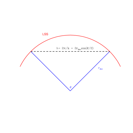
Figure 1: Angle-scale relation for CMB anisotropy.

On cosmological scales, the line element $ds^{2}=g_{\mu\nu}dx^{\mu}dx^{\nu}$ is described by a perturbed Friedmann Robertson Walker (FRW) metric tensor

$$g_{\mu\nu}(\vec{x},\eta)=a(\eta)^{2}[\gamma_{\mu\nu}+h_{\mu\nu}(\vec{x},\eta)]\ ,$$ (6)

where $a$ is the scale factor describing cosmic expansion and $\eta$ represents the conformal time, defined in terms of the usual time by $d\eta=dt/a$; $\gamma_{\mu\nu}$ represents he background Minkowski metric. The linear fluctuations $h_{\mu\nu}\ll 1$ are conveniently decomposed into the three different components

$$h_{\mu\nu}=h_{\mu\nu}^{S}+h_{\mu\nu}^{V}+h_{\mu\nu}^{T}\ ,$$ (7)

transforming as scalar, vector and tensor quantities under spatial rotations, respectively [8]. Scalar metric fluctuations represent, in a Newtonian fashion, scalar quantities like a gravitational potential; vectors modes represent vorticity while tensors represent cosmological gravitational waves. We restrict our analysis to scalar perturbations only. Linearity introduces a gauge freedom so that equations of motion and perturbed quantities can have different expressions in different frames separated by a linear coordinate transformation. In other words not all the elements of $h_{\mu\nu}$ are independent, but some of them can be set to zero via a proper gauge choice. Here we fix the conformal Newtonian gauge for which the metric fluctuations appear isotropic with respect to the cosmic expansion: the non-zero metric perturbations of scalar type are

$$\Psi={h_{00}\over 2}\ ,\ \Phi={h_{11}\over 2}={h_{22}\over 2}={h_{33}\over 2}\ .$$ (8)

On the other hand, linearity allows to analyze cosmological perturbation evolution in Fourier space, since Fourier modes do not mix at a linear level. Unless otherwise specified, we write equations in the Fourier space in the following.

Correspondingly to the metric fluctuations, the stress energy tensor $T_{\mu\nu}$ is perturbed: for what concerns scalar perturbations, any cosmological component $x$ admits energy density, velocity and pressure perturbations due to isotropic and anisotropic stress [8]:

$$\delta_{x}\equiv{\delta\rho_{x}\over\rho_{x}}\ ,\ v_{x}\ ,\ \pi_{L}\ ,\ \pi_{T}\ .$$ (9)

The above quantities fully describe scalar perturbations for non-relativistic species, for which velocity perturbations are enough to describe their peculiar motion with respect to the comoving expansion. Relativistic species move at the speed of light and are characterized by a propagation direction $\hat{n}$ which needs to be properly treated. The dependence on the propagation direction of the thermodynamical temperature of CMB photons is a key aspect of CMB perturbation phenomenology. Each Fourier component at wavevector $\vec{k}$, describing the spatial dependence, is expanded in the Fourier space, then the dependence on $\hat{n}$ is described through a spherical harmonic expansion taking the direction in the Fourier space, $\hat{k}$, as polar axis; for scalar perturbations, only Legendre polynomials are necessary [11]:

$${\delta T\over T}(\vec{k},\eta,\hat{n})=\sum_{l}\left({\delta T\over T}\right)_{l}(\eta)P_{l}(\hat{n}\cdot\hat{k})\ .$$ (10)

Monopole, dipole and quadrupole in the above expansion are related to density, velocity and stress perturbations of CMB radiation. In Newtonian gauge these relations, for density and velocity, take the form

$$\delta_{\gamma}=4\left({\delta T\over T}\right)_{0}\ ,\ v_{\gamma}=\left({\delta T\over T}\right)_{1}\ ,$$ (11)

where the first one recalls the Stephan-Boltzmann law $\rho\propto T^{4}$. As we expose in the next Section, most of the CMB phenomenology derives from the behavior of the monopole term.

Unperturbed Einstein equations link the Einstein gravitational tensor $G_{\mu\nu}$ to the stress energy tensor and describe the scale factor evolution. Conservation equations $T_{\mu;\nu}^{\nu}=0$ complete the evolution system. In the same way, perturbed Einstein and conservation equations describe perturbation evolution:

$$\delta G_{\mu\nu}=8\pi G\delta T_{\mu\nu}\ ,\ \delta T_{\mu\,;\nu}^{\nu}=0\ .$$ (12)

We do not write here the form of the above equations for all cosmological species. In the next Section we write only the ones which are relevant to give a simple understanding of the phenomenology of CMB anisotropies in terms of the initial conditions which are supposed to be fixed in the early Universe.

3 Sub-degree CMB acoustic oscillations

The dynamics of the CMB thermodynamical temperature fluctuations is dictated by the Thomson scattering cross section. For each Fourier mode, evolution equations for each multipole defined as in (10) can be expanded in power of the ratio between the wavevector amplitude $k$ and the differential optical depth for Thomson scattering $\dot{\tau}$, which corresponds to the inverse of the photon mean free path. Dynamics is frozen to the initial conditions for scales which are larger than cosmological horizon scale $\lambda_{H}$ and the photon mean free path, $k\lambda_{H}\ll 1$, $k/\dot{\tau}\ll 1$; generically, initial conditions are such that only the lowest multipoles are different from zero. After the horizon crossing these multipoles evolve giving rise to acoustic oscillations but do not transmit power to the higher multipoles until decoupling: at that time, the mean free path for photons increases rapidly up to the cosmological horizon and the oscillations are transmitted also to higher multipoles [10, 11]; therefore, the decoupled photons carry the snapshot of acoustic oscillations on sub-horizon scales at decoupling. Projected on the last scattering surface, the horizon corresponds to a degree in the sky, so that acoustic oscillations are mapped by sub-degree CMB anisotropies.

Figure 2: Schematical sketch of sub-horizon acoustic oscillations for Fourier modes having same wavenumber $k$ but different directions (top) and their mean quadratic power (middle); acoustic peaks in the sky signal in typical adiabatic cosmological models (bottom), see text.

For our purposes here, the study of the evolution of the zero-point fluctuation $(\delta T/T)_{0}$ is enough. At the lowest order in $k/\dot{\tau}$, after horizon crossing, neglecting the cosmological friction and the time derivatives of gravitational potentials, the zero-point temperature fluctuation obeys the simple equation

$$\ddot{\left({\delta T\over T}\right)}_{0}+{k^{2}\over 3}\left({\delta T\over T}\right)_{0}=-{k^{2}\over 3}\Psi\ ,$$ (13)

which merely represents an harmonic oscillator with radiation sound velocity $1/\sqrt{3}$, forced by the cosmological gravitational potential $\Psi$ [11]. In the limit in which the latter is constant, the solution, which is valid after the horizon crossing time $\eta_{HC}$, can be found analytically and describes most of the CMB acoustic oscillation phenomenology.

In the simplest inflationary scenario (see e.g. [1]) with adiabatic initial conditions, the curvature is perturbed with the same power on all cosmological scales at the horizon crossing. It can be seen [8] that curvature perturbation is closely related to the cosmological gravitational potential $\Psi$. Writing the generic Fourier mode as its module multiplied by its phase, $\Psi(\vec{k})=|\Psi(\vec{k})|e^{i\phi_{\vec{k}}}$, inflationary initial conditions generate an initial Gaussian spectrum where the first term has in mean the same amplitude for all modes at the horizon crossing, while the phase $\phi_{\vec{k}}$ is random.

At the horizon crossing the initial conditions for thermodynamical temperature fluctuations are simply related to the gravitational potential as

$$\left({\delta T\over T}\right)_{0}\propto\Psi\neq 0\ ,\ \dot{\left({\delta T\over T}\right)}_{0}=0\ ,$$ (14)

so that the solution to (13) takes the simple form

$$\left({\delta T\over T}\right)_{0}(\eta)=\left[\left({\delta T\over T}\right)_{0}(\eta_{HC})+\Psi\right] \times$$

$$\times\cos\left[{k(\eta-\eta_{HC})\over\sqrt{3}}\right]-\Psi\$$ , (15)

representing oscillation occurring for a given scale $k$; as it is schematically sketched in figure 2, $\delta T/T$ fluctuations for Fourier wavevectors with different direction but same amplitude $k$ have random phases so that their mean is zero but have the same zeros (top panel), and their root mean square power presents coherent acoustic peaks (middle panel) located at $k(\eta-\eta_{HC})=n\pi\sqrt{3}$, with $n$ integer. In the bottom panel, we show the sky signal of a typical cosmological model having adiabatic initial conditions. The highest peak corresponds to scales crossing the horizon just at decoupling, and occur at a multipole $l$ corresponding precisely to the angle subtended by the horizon at last scattering. The second peak at $l\simeq 500$ corresponds to scales that were in horizon crossing slightly before decoupling and that at the time of decoupling, when the CMB snapshot is taken, were in the maximum of their second oscillation. In the same way, the third peak corresponds to scales in horizon crossing even before, being in the maximum of their third oscillation at the moment of the snapshot. The series of peaks continues at higher multipoles, with decreasing amplitude because of diffusion damping.

As we mentioned in the Introduction, present data are strongly supporting this scenario, having revealed the first peak with very high confidence level and significant indications for a second and a third peak in the spectrum. Competing models for cosmological structure formation, see e.g. [1] and references therein, predict markedly different spectra. Isocurvature models are generally characterized by a non-zero entropy perturbation between different species, keeping the curvature unperturbed; consequently, at horizon crossing the zero-point temperature fluctuation is zero, but not its time derivative, resulting in a sine time dependence instead of a cosine like in adiabatic models (15), with a consequent shift of acoustic peaks by $\pi/2$ with respect to the adiabatic case. Coherent acoustic peaks are generally absent in non-Gaussian models like cosmological defects, because at horizon crossing both $(\delta T/T)_{0}$ and $(\delta T/T)_{1}$ can be different from zero, in a way which is different for each Fourier mode, thus destroying coherence.

In the next Section we conclude this paper, giving a worked example on how the evidence for acoustic peaks in the CMB spectrum and their sensitivity to the main cosmological parameters can be used to constrain cosmological models.

Figure 3: Likelihood peaks for Quintessence parameters $\Omega_{Q}$ (top) and $w_{Q}$ (bottom) showing preference for Quintessence models with $w_{Q}\simeq-0.8$.

4 Constraining dark energy with CMB data

As it is well known, CMB data are a powerful tool to constrain cosmological models, either because of the sensitivity on the most important cosmological parameters, either because they represent the Universe as it was before non-linear structure formation, thus being relatively simple to be read and understood. On the other hand, CMB alone cannot fix all cosmological parameters, either because of internal degeneracies [12], either because of the high number, about 10, of parameters to be investigated; independent datasets, mostly from Large Scale Structure (LSS) [13] and Type Ia supernovae [14] are needed in order to go deep in precision cosmology. However, under reasonable hypothesis, even the present CMB data, which of course do not reach the precision of the satellites MAP and Planck, can be used to derive interesting constraints on most important cosmological parameters.

Here we give an example of this, constraining a dynamical vacuum energy in flat cosmologies with the present CMB data. The dark energy, also known as Quintessence, occupies a central position in modern cosmology after that at least three independent evidences, LSS, Supernovae and CMB, gave indications that almost $70\%$ of the cosmological energy density today resides in a sort of vacuum energy which is responsible for the cosmic acceleration today [13, 14, 3, 4, 5]. To explain these observations a cosmological component with negative equation of state is necessary. Dark energy is described as a self-interacting scalar field rolling on its potential which admits dynamical trajectories, tracking solutions, in which its equation of state $w_{Q}$ can take values in the range [-0.5,-1], where the last value recovers the ordinary cosmological constant; these trajectories have been proved to exist both in ordinary and scalar-tensor cosmology (see e.g. [15] and references therein). The angle $\theta_{H}$ subtended by the horizon at decoupling is sensitive to the dark energy equation of state $w_{Q}$; indeed it is the ratio between the comoving value of Hubble horizon at decoupling, which is almost insensitive to values of $w_{Q}$ relevant for cosmic acceleration today, and the comoving distance of the last scattering surface from us, which is

$$\tau_{dec}\propto\int_{0}^{dec}dz[\Omega_{m}(1+z)^{3}+\Omega_{K}(1+z)^{2} +$$

$$+\Omega_{Q}(1+z)^{3(1+w_{Q})}]^{1/2}\$$ , (16)

where $\Omega_{m}$, $\Omega_{K}$ and $\Omega_{Q}$ represent matter, curvature and Quintessence present energy density, respectively. Therefore the angle subtended by the horizon at decoupling is essentially inversely proportional to $\tau_{dec}$. As it is evident, the expression above is degenerate in the sense that a given $\tau_{dec}$ can be made of different combinations of the parameters entering into the integral. However, one should remember that this is not the only effect of dark energy on CMB; the change in the equation of state at low redshift enhance the CMB power on low multipoles $l\leq 10$ and breaks the degeneracy between $\Omega_{Q}$ and $w_{Q}$ (see e.g. [15] and references therein). More serious is the degeneracy of dark energy with closed cosmological models with $\Omega_{K}>0$.

In our recent work [16] we fit CMB data [3, 4, 5] gridding several cosmological parameters as the baryon amount, cosmological gravitational waves and scalar spectral index, in addition to Quintessence parameters $\Omega_{Q}$ and $w_{Q}$, by assuming a number of priors including flatness $\Omega_{K}=0$. Interestingly, we find a preference of these data for dark energy models with respect to ordinary cosmological constant. This is shown in figure 3, representing the likelihood for $\Omega_{Q}$, peaking at $70\%$, and equation of state, peaking at $w_{Q}\simeq-0.8$. This effect can be understood as follows: best fits obtained in the original works on the CMB data [3, 4, 5] slightly prefer closed cosmological models, even if flatness is well within errors. As it is evident from the expression (16), dark energy models with $w_{Q}>-1$ induce a term which is similar to the one of closed models. Therefore, since we are assuming perfectly flat cosmologies, the best fit peak on dynamical vacuum energy models simply because they produce a similar geometrical effect on the angle subtended by the horizon at decoupling. Future data will help to test more deeply this interesting result.

References

- [1] A. Liddle and D.H. Lyth (eds.), Cosmological Inflation and Large Scale Structure, Cambridge University Press, 2000.
- [2] K.M. Gorski, Astrophys.J.S. 114 (1998) 1.
- [3] C. B. Netterfield et al., submitted to Astrophys.J (2001), preprint astro-ph/0104460.
- [4] A.T. Lee et al., submitted to Astrophys.J.Lett. (2001), preprint astro-ph/0104459.
- [5] N.W. Halverson et al., submitted to Astrophys.J. (2001), preprint astro-ph/0104489
- [6] P.J.E. Peebles and J.T. Yu, Astrophys.J. 162 (1970) 815.
- [7] J.M. Bardeen, Phys.Rev.D22 (1980) 1882.
- [8] I. Kodama and M. Sasaki, Progr. of Theor.Phys.Supp, 78 (1984), 1.
- [9] J.C. Hwang, Astrophys.J. 375 (1991) 443.
- [10] C.P. Ma and E. Bertschinger Astrophys.J. 455 (1995) 7.
- [11] W. Hu, U. Seljak, M. White, M. Zaldarriaga, Phys.Rev.D56 (1997) 596.
- [12] G. Efstathiou, submitted to MNRAS (2001), preprint astro-ph/0109151.
- [13] J.A. Peacock et at., Nature 410 (2001) 169
- [14] S. Perlmutter et at., Astrophys.J. 517 (1999) 565; A. Riess et al., Astron.J. 116 (1998) 1009.
- [15] C. Baccigalupi, S. Matarrese, F. Perrotta Phys.Rev.D62 (2000) 123510.
- [16] C. Baccigalupi, A. Balbi, S. Matarrese, F. Perrotta, N. Vittorio, submitted to Phys.Rev.D (2001), preprint astro-ph/0109097.