Cosmic String Signatures in the Cosmic Microwave Background Anisotropies

Abstract

We briefly review certain aspects of cosmic microwave background anisotropies as generated in passive and active models of structure formation. We then focus on cosmic strings based models and discuss their status in the light of current high-resolution observations from the BOOMERanG, MAXIMA and DASI collaborations. Upcoming megapixel experiments will have the potential to look for non-Gaussian features in the CMB temperature maps with unprecedented accuracy. We therefore devote the last part of this review to treat the non-Gaussianity of the microwave background and present a method for computation of the bispectrum from simulated string realizations.

1 Introduction

Anisotropies of the Cosmic Microwave Background radiation (CMB) are directly related to the origin of structure in the universe. Galaxies and clusters of galaxies eventually formed by gravitational instability from primordial density fluctuations, and these same fluctuations left their imprint on the CMB. Recent balloon boomerang ; maxima and ground-based interferometer dasi experiments have produced reliable estimates of the power spectrum of the CMB temperature anisotropies. While they helped eliminate certain candidate theories for the primary source of cosmic perturbations, the power spectrum data are still compatible with theoretical estimates of a relatively large variety of models, such as $\Lambda$CDM, quintessence models or some hybrid models including cosmic defects. These models, however, differ in their predictions for the statistical distribution of the anisotropies beyond the power spectrum. The MAP (currently in space) and Planck (scheduled for launch in 2007) satellite missions will provide high-precision data allowing definite estimates of non-Gaussian signals in the CMB. It is therefore important to know precisely what are the predictions of all candidate models for the statistical quantities that will be extracted from the new data, and to identify specific signatures of the various models.

There are two main classes of models of structure formation—passive and active models. In passive models, density inhomogeneities are set as initial conditions at some early time, and while they subsequently evolve as described by Einstein-Boltzmann equations, no additional perturbations are seeded. On the other hand, in active models a time-dependent source generates new density perturbations through all time.

Most realizations of passive models are based on the idea of inflation. In simplest inflationary models it is assumed that there exists a weakly coupled scalar field $\phi$, called the inflaton, which “drives” the (approximately) exponential expansion of the universe. Quantum fluctuations of $\phi$ are stretched by the expansion to scales beyond the horizon, thus “freezing” their amplitude. Inflation is followed by a period of thermalization, or reheating, during which energy is transferred to usual particles. Because of the spatial variations of $\phi$ introduced by quantum fluctuations, thermalization occurs at slightly different times in different parts of the universe. Such fluctuations in the thermalization time give rise to density fluctuations. Because of their quantum nature and because of the fact that initial perturbations are assumed to be in the vacuum state and hence well described by a Gaussian distribution, perturbations produced during inflation are expected to follow Gaussian statistics to a high degree, or either be products of Gaussian random variables. This is a fairly general prediction that will be tested shortly with MAP and more thoroughly in the future with Planck data.

Active models of structure formation are motivated by cosmic topological defects with the most promising candidates being cosmic strings. It is widely believed that the universe underwent a series of phase transitions as it cooled down due to the expansion. If our ideas about grand unification are correct, then some cosmic defects, such as domain walls, strings, monopoles or textures, should have formed during phase transitions in the early universe vilshel . Once formed, cosmic strings could survive long enough to seed density perturbations. Generically, perturbations produced by active models are not expected to be Gaussian.

Defect models possess the attractive feature that they have no parameter freedom, as all the necessary information is in principle contained in the underlying particle physics model. This is a feature that fascinated Dennis Sciama: during his days at Trieste, he would always be willing to discuss these “marvelous cosmic defects” with everyone. He even encouraged a few students sans liaisons contraignantes to pursue studies on this promising subject and facilitated all necessary means for it. The relevant, ubiquitous dimensionless quantity for every astrophysical and cosmological signature left by strings is $G\mu$, where $G$ is Newton’s constant and $\mu$ stands for the mass per unit length of the string, with a value of roughly $G\mu\sim 10^{-6}$ for GUT strings. This happens to be just the correct order of magnitude of the level of CMB anisotropies. Back in 1996, the power spectrum plot of $l(l+1)C_{l}$ vs. $l$ consisted of some scattered points and strings were considered a likely candidate for the origin of structure formation. Moreover, the error bars were so big that Dennis would never miss the opportunity to tease inflation fans who wanted to see a peak in that plot: “Come on”, he would say, “you do not claim you actually see a peak there, do you..!”.

To close this section, let us mention that, in addition to purely active or passive scenarios, perturbations could be seeded by some combination of the two mechanisms. For example, cosmic strings could have formed just before the end of inflation and partially contributed to seeding density fluctuations. It has been shown hybrid that such hybrid models are very successful in fitting the CMB power spectrum data. Cosmic strings are generally expected to produce distinguishing non-Gaussian features in the CMB and it will soon become possible to look for them in the data from MAP and Planck.

2 CMB power spectrum from strings

Calculating CMB anisotropies sourced by topological defects is a rather difficult task. In inflationary scenario the entire information about the seeds is contained in the initial conditions for the perturbations in the metric. In the case of cosmic defects, perturbations are continuously seeded over the period of time from the phase transition that had produced them until today. The exact determination of the resulting anisotropy requires, in principle, the knowledge of the energy-momentum tensor [or, if only two point functions are being calculated, the unequal time correlators uetc ] of the defect network and the products of its decay at all times. This information is simply not available! Instead, a number of clever simplifications, based on the expected properties of the defect networks (e.g. scaling), are used to calculate the source. The latest data from BOOMERanG boomerang , MAXIMA maxima and DASI dasi experiments clearly disagree with the predictions of these simple models of defects dgs96 .

The shape of the CMB angular power spectrum is determined by three main factors: the geometry of the universe, coherence and causality.

The curvature of the universe directly affects the paths of light rays coming to us from the surface of last scattering weinberg . In a closed universe, because of the lensing effect induced by the positive curvature, the same physical distances between points on the sky would correspond to larger angular scales. As a result, the peak structure in the CMB angular power spectrum would shift to the larger angular scales or the smaller values of $l$.

The prediction of the cosmic string model of PV99 for $\Omega_{\rm total}=1.3$ is shown in Fig. 1.

Figure 1: Data from BOOMERanG (solid error bars), MAXIMA (dotted error bars) and DASI (dashed error bars). The line shows the CMB power spectrum produced by the wiggly local string model of Ref. PV99 in a closed universe with $\Omega_{\rm total}=1.3$, $\Omega_{\rm baryon}=0.05$, $\Omega_{\rm CDM}=0.35$, $\Omega_{\Lambda}=0.9$, and $H_{0}=65{\rm~{}km~{}s}^{-1}{\rm Mpc}^{-1}$.

As can be seen, the main peak in the angular power spectrum can be matched by choosing a reasonable value for $\Omega_{\rm total}$. However, even with the main peak in the right place the agreement with the data is far from satisfactory. The peak is significantly wider than that in the data and there is no sign of a rise in power at $l\approx 600-800$ suggested by the data. The situation is even worse for global strings which fail to produce a distinct peak of any kind. For local strings, the sharpness and the height of the main peak in the angular spectrum can be enhanced by including the effects of the gravitational radiation hind98 and wiggles PV99 . More precise high-resolution numerical simulations of string networks in realistic cosmologies with a large contribution from $\Omega_{\Lambda}$ are needed to determine the exact amount of small-scale structure on the strings and the nature of the products of their decay. It is, however, unlikely that including these effects alone would result in a sufficiently narrow main peak or any presence of secondary peaks. It seems that now Dennis would not have had strong arguments to tease his friends.

Let us next consider issues of causality and coherence and how the random nature of the string networks comes into the calculation of the anisotropy spectrum.

Both experimental and theoretical results for the CMB power spectra involve calculations of averages. To estimate the correlations of the observed temperature anisotropies, experimentalists compute the average over all available patches on the sky. When calculating the predictions of their models, theorists find the average over the ensemble of possible outcomes provided by the model.

In inflationary models, as in all passive models, only the initial conditions for the perturbations are random. The subsequent evolution is the same for all members of the ensemble. For wavelengths higher than the Hubble radius, the linear evolution equations for the Fourier components of such perturbations have a growing and a decaying solution. The modes corresponding to smaller wavelengths have only oscillating solutions. As a consequence, prior to entering the horizon, each mode undergoes a period of phase “squeezing” which leaves it in a highly coherent state by the time it starts to oscillate. Coherence here means that all members of the ensemble, corresponding to the same Fourier mode, have the same temporal phase. So even though there is randomness involved, as one has to draw random amplitudes for the oscillations of a given mode, the time behavior of different members of the ensemble is highly correlated. The total power spectrum is an ensemble averaged superposition of all Fourier modes and the coherence results in an interference pattern seen as the acoustic peaks.

Figure 2: Predictions of the toy model of Magueijo et al. mag&alb for different values of parameters $x_{c}$, the coherence length, and $\tau_{c}$, the coherence time; $x_{c}\propto\eta/\lambda_{c}(\eta)$, where $\eta$ is the conformal time and $\lambda_{c}(\eta)$ is the correlation length of the network at time $\eta$. One can obtain oscillations in the CMB power spectrum by fixing either one of the parameters and varying the other.

In contrast, the evolution of the string network is highly non-linear. Cosmic strings are expected to move at relativistic speeds, self-intersect and reconnect in a chaotic fashion. A consequence of this behavior is that the unequal time correlators of the string energy-momentum vanish for time differences larger than a certain coherence time. Members of the ensemble corresponding to a given mode of perturbations will have random temporal phases with the “dice” thrown on average once in each coherence time. The coherence time of a realistic string network is rather short. As a result, the interference pattern in the angular power spectrum is completely washed out.

Causality manifests itself, first of all, through the initial conditions for the string sources, the perturbations in the metric and the densities of different particle species. If one assumes that defects are formed by a causal mechanism in an otherwise smooth universe, then the correct initial conditions are obtained by setting the components of the stress-energy pseudo-tensor $\tau_{\mu\nu}$ to zero veersteb ; PenSperTur . These are the same as the isocurvature initial conditions HuSperWhite . A generic prediction of isocurvature models (assuming perfect coherence) is that the first acoustic peak is almost completely hidden. The main peak is then the second acoustic peak and in flat geometries it appears at $l\approx 300-400$. This is due to the fact that after entering the horizon a given Fourier mode of the source perturbation requires time to induce perturbations in the photon density.

Causality also implies that no superhorizon correlations in the string energy density are allowed. The correlation length of a “realistic” string network is normally between 0.1 and 0.4 of the horizon size.

An interesting study was performed by Magueijo et al. mag&alb where they have constructed a toy model of defects with two parameters: the coherence length and the coherence time. The coherence length was taken to be the scale at which the energy density power spectrum of the strings turns from a power law decay for large values of $k$ into a white noise at low $k$. This is essentially the scale corresponding to the correlation length of the string network. The coherence time was defined in the sense described in the beginning of this section, in particular, as the time difference needed for the unequal time-correlators to vanish. Their study showed (see Fig. 2) that by accepting any value for one of the parameters and varying the other (within the constraints imposed by causality) one could reproduce the oscillations in the CMB power spectrum. Unfortunately for cosmic strings, at least as we know them today, they fall into the parameter range corresponding to the upper right corner in Fig. 2. In order to fit the observations, cosmic strings must either be more coherent or they have to be stretched over larger distances, which is another way of making them more coherent. To understand this, imagine that there were only one long straight string stretching across the universe and moving with some velocity. The evolution of this string would be linear and the induced perturbations in the photon density would be coherent. By increasing the correlation length of the string network we would move closer to this limiting case of just one long straight string and so the coherence would be enhanced.

Figure 3: $\ell(\ell+1)C_{\ell}$ versus $\ell$ for three different models [the figure is borrowed from Bouchet et al., Ref. hybrid ]. The upper (dot-dashed) line represents the prediction of a $\Lambda$CDM model, with $n_{\rm S}=1$, $\Omega_{\Lambda}=0.7$, $\Omega_{\rm m}=0.3$, $\Omega_{\rm b}=0.05$ and $h=0.6$. The lower dashed line is a typical spectrum produced by global strings. Both lines are normalized at the COBE scale (crosses). Combining both curves, with their relative contribution as a free parameter, produces the solid curve. The string contribution is about 18% of the total.

The question of whether or not defects can produce a pattern of the CMB power spectrum similar to, and including the peaks of, that produced by the adiabatic inflationary models was repeatedly addressed in the literature hybrid ; mag&alb ; liddle ; turok ; varyingc . In particular, it was shown mag&alb ; turok that one can construct a causal model of active seeds which for certain values of parameters can reproduce the oscillations in the CMB spectrum. The main problem today is that current realistic models of cosmic strings fall out of the parameter range that is needed to fit the observations.

In addition to purely active or passive models, perturbations could be seeded by some combination of the two mechanisms hybrid . Figure 3 (borrowed from Bouchet et al.) shows two uncorrelated spectra produced by an inflationary $\Lambda$CDM model (dot-dashed line) and a global string model (dashed line), both normalized on the COBE data, as well as a weighted sum of the two (solid line). The best fit to the latest BOOMERanG, MAXIMA and DASI data is obtained with a non-negligible string contribution of $18$%. At the moment, models combining strings with inflation hybrid or models of varying speed of light varyingc are the only ones involving topological defects that to some extent can match the observations. One possible way to distinguish their predictions from those of inflationary models would be to compute a non-Gaussian statistic, such as the CMB bispectrum.

3 CMB Bispectrum from strings

3.1 The string model

Let us now turn to a computation of the bispectrum of CMB temperature anisotropies as generated by simulated cosmic strings. To calculate the sources of perturbations we use an updated version of the wiggly string model of Ref.PV99 (see also ABR97 ).

The network is represented by a collection of uncorrelated, straight string segments moving with random, uncorrelated velocities, and are produced at some early epoch. At every subsequent epoch, a certain fraction of the number of segments decays in a way that maintains network scaling. The length of each segment at any time is taken to be equal to the correlation length of the network which, together with the root mean square velocity of segments, are computed from the velocity-dependent one-scale model of Martins and Shellard MS00 ; MS96 . The positions of segments are drawn from a uniform distribution in space and their orientations are chosen from a uniform distribution on a two-sphere.

According to the one-scale model Kib ; Ben ; MS96 ; MS00 , the string network at any time can be characterized by a single length scale, the correlation length $L$, defined by $\rho={\mu}/{L^{2}}$, where $\rho$ is the energy density in the string network. Expansion of space stretches the strings without altering their mass per unit length. If simply stretched in that manner, strings would soon come to dominate the energy density of the universe. However, at the same time with the expansion, long strings reconnect and chop off loops which later decay. These two competing effects result in an intermediate steady-state (the so-called “scaling solution”) in which the characteristic scale of the string network remains constant relative to the horizon size.

The total energy of the string network in a volume $V$ at any time $\tau$ is

$$N\mu L=V\rho=\frac{\mu V}{L^{2}}$$ (1)

where $N=N(\tau)$ is the total number of string segments at that time, $V=V_{0}a^{3}$, $a$ is the expansion factor and $V_{0}$ is a constant simulation volume. From Eq.(1) it follows that $N={V}/{L^{3}}={V_{0}}/{{\ell}^{3}}$, where we have defined ${\ell}\equiv L/a$. The comoving length ${\ell}$ is approximately proportional to the conformal time $\tau$ and implies that the number of strings $N(\tau)$ within the simulation volume $V_{0}$ falls as $\tau^{-3}$. To calculate the CMB anisotropy we need to evolve the string network over at least four orders of magnitude in cosmic expansion. Hence we would have to start with $N\geq 10^{12}$ string segments in order to have one segment left at the present time. Keeping track of such a large number of segments is numerically impossible. Fortunately, a way around this difficulty was suggested in Ref. ABR97 .

The suggestion is to consolidate all string segments that decay at the same epoch. The number of segments that decay at the (discretized) conformal time $\tau_{i}$ is

$$N_{d}(\tau_{i})=V[n(\tau_{i-1})-n(\tau_{i})]$$ (2)

where $n(\tau)=[\ell(\tau)]^{-3}$ is the number density of strings at time $\tau$. Then, with the formalism we employ, instead of summing over $\sum_{i=1}^{K}N_{d}(\tau_{i})\geq 10^{12}$ segments we now sum over only $K$ segments, making $K$ a parameter. Such a simplification only works for computation of two- and three-point correlation functions under the assumption that string segments are statistically independent. We refer the interested reader to our recent article usthree , where we explain the procedure in more detail.

As a final comment, let us note that the simulation model in this form does not allow computation of CMB sky maps. This is because the method of finding the two- and three-point functions we describe involves “consolidated” quantities which do not correspond to the energy-momentum tensor of a real string network. These quantities are auxiliary and specially prepared to give the correct two- or three-point functions after ensemble averaging. Having clarified this, the stress-energy from the simulated string model can be found and used to compute the appropriate density perturbations which lead to the expected CMB temperature anisotropies.

3.2 Computation of bispectrum from string realizations

It is conventional to expand CMB temperature fluctuations into spherical harmonics:

$${\Delta T/T}({\bf e})=\sum_{lm}a_{lm}Y_{lm}({\bf e}).$$ (3)

The coefficients $a_{lm}$ can be decomposed into Fourier modes,

$$a_{lm}=\frac{V_{0}}{(2\pi)^{3}}\left(-i\right)^{l}4\pi\int d^{3}{\mathbf{k}}\,\Delta_{l}\left({\mathbf{k}}\right)Y^{*}_{lm}(\hat{{\mathbf{k}}}).$$ (4)

Given the sources $\Theta_{\mu\nu}({\mathbf{k}},\tau)$ produced by the string model, $\Delta_{l}({\mathbf{k}})$ are found by solving linearized Einstein-Boltzmann equations and integrating along the line of sight cmbfast . This procedure can be written as the action of a linear operator ${\hat{B}}_{l}^{\mu\nu}(k)$ on the source energy-momentum tensor, $\Delta_{l}({\mathbf{k}})={\hat{B}}_{l}^{\mu\nu}(k)\Theta_{\mu\nu}({\mathbf{k}},\tau)$. The third moment of $a_{lm}$’s can be expressed as

$$\left\langle a_{l_{1}m_{1}}a_{l_{2}m_{2}}a_{l_{3}m_{3}}\right\rangle = \left(-i\right)^{l_{1}+l_{2}+l_{3}}\left(4\pi\right)^{3}\!\!\frac{V_{0}^{3}}{(2\pi)^{9}}\!\!\int\!\!d^{3}{\mathbf{k}}_{1}d^{3}{\mathbf{k}}_{2}d^{3}{\mathbf{k}}_{3}Y^{*}_{l_{1}m_{1}}\!(\hat{{\mathbf{k}}}_{1})$$ (5)

$$\times Y^{*}_{l_{2}m_{2}}\!(\hat{{\mathbf{k}}}_{2})Y^{*}_{l_{3}m_{3}}\!(\hat{{\mathbf{k}}}_{3})\left\langle\Delta_{l_{1}}\!\!\left({\mathbf{k}}_{1}\right)\Delta_{l_{2}}\!\!\left({\mathbf{k}}_{2}\right)\Delta_{l_{3}}\!\!\left({\mathbf{k}}_{3}\right)\right\rangle.$$

Because of homogeneity we have

$$\left\langle\Delta_{l_{1}}\left({\mathbf{k}}_{1}\right)\Delta_{l_{2}}\left({\mathbf{k}}_{2}\right)\Delta_{l_{3}}\left({\mathbf{k}}_{3}\right)\right\rangle=\delta^{(3)}\left({\mathbf{k}}_{1}+{\mathbf{k}}_{2}+{\mathbf{k}}_{3}\right)P_{l_{1}l_{2}l_{3}}\left({\mathbf{k}}_{1},{\mathbf{k}}_{2},{\mathbf{k}}_{3}\right).$$ (6)

Given scalar values $k_{1}$, $k_{2}$, $k_{3}$, there is a unique (up to an overall rotation) triplet of directions $\hat{{\mathbf{k}}}_{i}$ for which the RHS of Eq. (6) does not vanish. The quantity $P_{l_{1}l_{2}l_{3}}\left({\mathbf{k}}_{1},{\mathbf{k}}_{2},{\mathbf{k}}_{3}\right)$ is invariant under an overall rotation of all three vectors ${\mathbf{k}}_{i}$ and therefore may be equivalently represented by a function of scalar values $k_{1}$, $k_{2}$, $k_{3}$. Hence, we get

$$\left\langle\Delta_{l_{1}}\left({\mathbf{k}}_{1}\right)\Delta_{l_{2}}\left({\mathbf{k}}_{2}\right)\Delta_{l_{3}}\left({\mathbf{k}}_{3}\right)\right\rangle=\delta^{(3)}\left({\mathbf{k}}_{1}+{\mathbf{k}}_{2}+{\mathbf{k}}_{3}\right)P_{l_{1}l_{2}l_{3}}(k_{1},k_{2},k_{3}).$$ (7)

The triangle constraint ${\mathbf{k}}_{1}+{\mathbf{k}}_{2}+{\mathbf{k}}_{3}=0$ must be satisfied. Then, in terms of the simulation volume $V_{0}$, we have

$$P_{l_{1}l_{2}l_{3}}\!\left(k_{1},k_{2},k_{3}\right)\!=\!\frac{(2\pi)^{3}}{V_{0}}\left\langle\Delta_{l_{1}}\!\!\left({\mathbf{k}}_{1}\right)\Delta_{l_{2}}\!\!\left({\mathbf{k}}_{2}\right)\Delta_{l_{3}}\!\!\left({\mathbf{k}}_{3}\right)\right\rangle.$$ (8)

Given an arbitrary direction $\hat{\mathbf{k}}_{1}$ and the magnitudes $k_{1}$, $k_{2}$ and $k_{3}$, the directions $\hat{\mathbf{k}}_{2}$ and $\hat{\mathbf{k}}_{3}$ are specified up to rotations by the triangle constraint. Both sides of Eq. (8) are function of scalar $k_{i}$ only. The expression on the RHS will be computed numerically by averaging over different realizations of the string network and over all directions $\hat{\mathbf{k}}_{1}$. Because of isotropy and since the allowed sets of directions $\hat{\mathbf{k}}_{i}$ are planar, it is enough to restrict the numerical calculation to directions $\hat{\mathbf{k}}_{i}$ in a fixed plane. This significantly reduces the computational expense.

Substituting Eqs. (6) to (8) into (5), Fourier transforming the Dirac delta and using the Rayleigh identity, we can perform all angular integrations analytically and obtain a compact form for the third moment

$$\left\langle a_{l_{1}m_{1}}a_{l_{2}m_{2}}a_{l_{3}m_{3}}\right\rangle={\mathcal{H}}_{l_{1}l_{2}l_{3}}^{m_{1}m_{2}m_{3}}\int r^{2}dr\,b_{l_{1}l_{2}l_{3}}(r),$$ (9)

where, noting $\left({}^{\,\,l_{1}~{}\,\;l_{2}~{}\,\;l_{3}}_{m_{1}~{}m_{2}~{}m_{3}}\right)$ a Wigner 3$j$-symbol, we have

$${\mathcal{H}}_{l_{1}l_{2}l_{3}}^{m_{1}m_{2}m_{3}} \equiv \sqrt{\frac{\left(2l_{1}+1\right)\left(2l_{2}+1\right)\left(2l_{3}+1\right)}{4\pi}}\left(\begin{array}[]{ccc}l_{1}&l_{2}&l_{3}\\ 0&0&0\end{array}\right)\left(\begin{array}[]{ccc}l_{1}&l_{2}&l_{3}\\ m_{1}&m_{2}&m_{3}\end{array}\right)\,,$$ (14)

and where we have defined, in terms of spherical Bessel functions $j_{l}$,

$$b_{l_{1}l_{2}l_{3}}(r) \equiv \frac{8}{\pi^{3}}\frac{V_{0}^{3}}{(2\pi)^{3}}\int k_{1}^{2}dk_{1}\,k_{2}^{2}dk_{2}\,k_{3}^{2}dk_{3}\,$$ (15)

$$\times j_{l_{1}}(k_{1}r)j_{l_{2}}(k_{2}r)j_{l_{3}}(k_{3}r)P_{l_{1}l_{2}l_{3}}(k_{1},k_{2},k_{3}).$$

Our numerical procedure consists of computing the RHS of Eq. (9) by evaluating the necessary integrals and averaging over many realizations of the strings sources. Readers wishing more details can consult Ref. usthree .

From Eq. (9) we easily derive the CMB bispectrum ${\mathcal{C}}_{l_{1}l_{2}l_{3}}$, defined as GM00

$$\bigl{\langle}a_{l_{1}m_{1}}a_{l_{2}m_{2}}a_{l_{3}m_{3}}\bigr{\rangle}=\left(\begin{array}[]{ccc}l_{1}&l_{2}&l_{3}\\ m_{1}&m_{2}&m_{3}\end{array}\right){\mathcal{C}}_{l_{1}l_{2}l_{3}}\,.$$ (18)

We now restrict our calculations to the angular bispectrum $C_{l_{1}l_{2}l_{3}}$ in the ‘diagonal’ case, i.e. $l_{1}=l_{2}=l_{3}=l$. This is a representative case and, in fact, the one most frequently considered in the literature. The power spectrum is usually plotted in terms of $l(l+1)C_{l}$ which, apart from constant factors, is the contribution to the mean squared anisotropy of temperature fluctuations per unit logarithmic interval of $l$. In full analogy with this, the relevant quantity to work with in the case of the bispectrum is

$$G_{lll}=l(2l+1)^{3/2}\left(\begin{array}[]{ccc}l&l&l\\ 0&0&0\end{array}\right)C_{lll}\,.$$ (21)

For large values of the multipole index $l$, $G_{lll}\propto l^{3/2}C_{lll}$. Note also what happens with the 3$j$-symbols appearing in the definition of the coefficients ${\mathcal{H}}_{l_{1}l_{2}l_{3}}^{m_{1}m_{2}m_{3}}$: the symbol $\left({}^{\,\,l_{1}\,\;l_{2}\,\;l_{3}}_{m_{1}m_{2}m_{3}}\right)$ is absent from the definition of $C_{l_{1}l_{2}l_{3}}$, while in Eq. (21) the symbol $\left({}^{\,l\;l\;l}_{0\>0\>0}\right)$ is squared. Hence, there are no remnant oscillations due to the alternating sign of $\left({}^{\,l\;l\;l}_{0\>0\>0}\right)$.

However, even more important than the value of $C_{lll}$ itself is the relation between the bispectrum and the cosmic variance associated with it. In fact, it is their comparison that tells us about the observability ‘in principle’ of the non-Gaussian signal. The cosmic variance constitutes a theoretical uncertainty for all observable quantities and is due to having just one realization of the stochastic process, in our case, the CMB sky.

The way to proceed is to employ an estimator $\hat{C}_{l_{1}l_{2}l_{3}}$ for the bispectrum and compute the variance from it. By choosing an unbiased estimator we ensure it satisfies $C_{l_{1}l_{2}l_{3}}=\langle\hat{C}_{l_{1}l_{2}l_{3}}\rangle$. However, this condition does not isolate a unique estimator. The proper way to select the best unbiased estimator is to compute the variances of all candidates and choose the one with the smallest value. The estimator with this property was computed in Ref. GM00 and is

$$\hat{C}_{l_{1}l_{2}l_{3}}=\!\!\!\sum_{m_{1},m_{2},m_{3}}\!\!\left(\begin{array}[]{ccc}l_{1}&l_{2}&l_{3}\\ m_{1}&m_{2}&m_{3}\end{array}\right)a_{l_{1}m_{1}}a_{l_{2}m_{2}}a_{l_{3}m_{3}}.$$ (22)

The variance of this estimator, assuming a mildly non-Gaussian distribution, can be expressed in terms of the angular power spectrum $C_{l}$ as follows GM00

$$\sigma^{2}_{\hat{C}_{l_{1}l_{2}l_{3}}}\!\!\!\!=C_{l_{1}}C_{l_{2}}C_{l_{3}}\!\left(1\!+\!\delta_{l_{1}l_{2}}\!\!+\!\delta_{l_{2}l_{3}}\!\!+\!\delta_{l_{3}l_{1}}\!\!+\!2\delta_{l_{1}l_{2}}\delta_{l_{2}l_{3}}\right).$$ (23)

The theoretical signal-to-noise ratio for the bispectrum (in the diagonal case $l_{1}=l_{2}=l_{3}=l$) is then given by

$$(S/N)_{l_{1}l_{2}l_{3}}=|C_{l_{1}l_{2}l_{3}}/\sigma_{\hat{C}_{l_{1}l_{2}l_{3}}}|.$$ (24)

Incorporating all the specifics of the particular experiment, such as sky coverage, angular resolution, etc., will allow us to give an estimate of the particular non-Gaussian signature associated with a given active source and, if observable, indicate the appropriate range of multipole $l$’s where it is best to look for it.

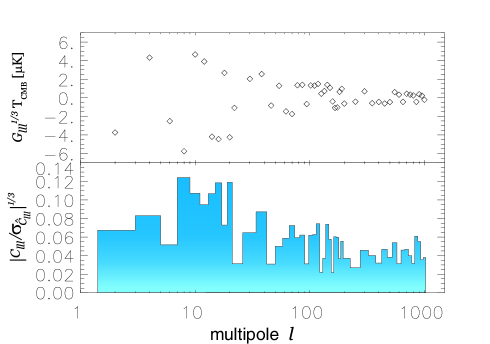
Figure 4: The CMB angular bispectrum in the ‘diagonal’ case ($G_{lll}^{1/3}$) from wiggly cosmic strings in a spatially flat model with cosmological parameters $\Omega_{\textrm{CDM}}=0.3$, $\Omega_{\textrm{baryon}}=0.05$, $\Omega_{\Lambda}=0.65$, and Hubble constant $H=0.65{\textrm{km}}{\textrm{s}}^{-1}{\textrm{Mpc}}^{-1}$ [upper panel]. In the lower panel we show the ratio of the signal to theoretical noise $|C_{lll}/\sigma_{\hat{C}_{lll}}|^{1/3}$ for different multipole indices. Normalization follows from fitting the power spectrum to the BOOMERanG and MAXIMA data.

In Fig. 4 we show the results for $G_{lll}^{1/3}$ [cf. Eq. (21)]. It was calculated using the string model with $800$ consolidated segments in a flat universe with cold dark matter and a cosmological constant. Only the scalar contribution to the anisotropy has been included. Vector and tensor contributions are known to be relatively insignificant for local cosmic strings and can safely be ignored in this model ABR97 ; PV99 . The plots are produced using a single realization of the string network by averaging over $720$ directions of ${\mathbf{k}}_{i}$. The comparison of $G_{lll}^{1/3}$ (or equivalently ${C}_{lll}^{1/3}$) with its cosmic variance [cf. Eq. (23)] clearly shows that the bispectrum (as computed from our cosmic string model) lies hidden in the theoretical noise and is therefore undetectable for any given value of $l$.

Let us note, however, that in its present stage our string code describes Brownian, wiggly long strings in spite of the fact that long strings are very likely not Brownian on the smallest scales. In addition, the presence of small string loops proty and gravitational radiation into which they decay were not yet included in our model. These are important effects that could, in principle, change our predictions for the string-generated CMB bispectrum on very small angular scales.

4 Outlook

The imprint of cosmic strings on the CMB is a combination of different effects. Prior to the time of recombination strings induce density and velocity fluctuations on the surrounding matter. During the period of last scattering these fluctuations are imprinted on the CMB through the Sachs-Wolfe effect: namely, temperature fluctuations arise because relic photons encounter a gravitational potential with spatially dependent depth. In addition to the Sachs-Wolfe effect, moving long strings drag the surrounding plasma and produce velocity fields that cause temperature anisotropies due to Doppler shifts. While a string segment by itself is a highly non-Gaussian object, fluctuations induced by string segments before recombination are a superposition of effects of many random strings stirring the primordial plasma. These fluctuations are thus expected to be Gaussian as a result of the central limit theorem.

As the universe becomes transparent, strings continue to leave their imprint on the CMB mainly due to the Kaiser-Stebbins effect. This effect creates line discontinuities in the temperature field of photons passing on opposite sides of a moving long string. However, this effect can produce non-Gaussian perturbations only on sufficiently small scales. This is because on scales larger than the characteristic inter-string separation at the time of the radiation-matter equality, the CMB temperature perturbations result from superposition of effects of many strings and are likely to be Gaussian.

Currently, strongest constraints on cosmic string models come from the CMB power spectrum data. Predictions of strings-only models are inconsistent with data from BOOMERanG, MAXIMA and DASI. However, the data can still be fitted reasonably well by “hybrid” models that combine strings and adiabatic inflationary perturbations as sources for primordial fluctuations. Presence of cosmic strings could, in principle, be distinguished by non-Gaussian statistics. The new high-resolution CMB measurements from MAP and PLANCK will allow a precise estimate of non-Gaussian signals in the CMB.

The most straightforward non-Gaussian discriminator is the three-point function of temperature, or equivalently (in Fourier space) the angular bispectrum. In Ref. usthree , we have developed a numerical method for computing the CMB angular bispectrum from first principles in any active model of structure formation, such as cosmic defects, where the energy-momentum tensor is known or can be simulated. The method does not use CMB sky maps and requires a moderate amount of computations. We applied this method to the computation of some relevant components of the bispectrum produced from a model of cosmic strings and did not find a non-Gaussian signal that would be observable in the forthcoming satellite-based CMB missions. This indicates that either the model we used to simulate cosmic strings is inadequate for extracting the non-Gaussian signature, or that the angular bispectrum is not an appropriate statistic for detecting cosmic strings.

Avelino et al. ASWA98 applied several non-Gaussian tests to the perturbations seeded by cosmic strings. They found the density field distribution to be close to Gaussian on scales larger than $1.5(\Omega_{M}h^{2})^{-1}$ Mpc, where $\Omega_{M}$ is the fraction of cosmological matter density in baryons and CDM combined. Scales this small correspond to the multipole index of order $l\sim 10^{4}$. We have not attempted a calculation the CMB bispectrum on these scales because the linear approximation is almost guaranteed to fail at such small scales, and because of increased computational cost for higher $l$ multipoles.

The interest in cosmic strings has considerably declined since they have been ruled out as the primary seed for structure formation in the universe. This, however, is not at all sufficient to rule out strings as an interesting topic of research. Studying formation, evolution, properties and cosmological implications of cosmics strings and other topological defects remains to be both exciting and important. Certain cosmological puzzles, such as baryogenesis and ultra-high energy cosmic rays, could be resolved with the help of topological defects vilshel . Recent experimental and theoretical progress in understanding properties of topological defects in low-temperature condensed matter systems, such as superfluid helium and superconductors, has led to an intriguing possibility of studying Cosmology in the Lab grisha . Any new experimental constraint on the population and properties of cosmic defects is potentially relevant to building viable cosmological and particle physics models. Since current and future CMB experiments will provide the most precise cosmological data, it is absolutely essential to use them maximally in learning as much as we can about cosmic defects.

 

me voy por un camino de labores fecundas,
a mi muerte yunques tañed, callad campanas

References

- (1) P. de Bernardis, et al., Nature 404, 995 (2000); preprint astro-ph/0004404; C. B. Netterfield, et al., preprint astro-ph/0104460.
-
(2)
S. Hanany, et al., Astrophys. J. 545 (2000) L5; preprint astro-ph/0005123;
A.H. Jaffe, et al., Phys. Rev. Lett. 86 (2001) 3475-3479; preprint astro-ph/0007333; A. T. Lee, et al., preprint astro-ph/0104459. - (3) N. W. Halverson, et al., preprint astro-ph/0104489.
-
(4)
A. Vilenkin, E.P.S. Shellard, “Cosmic Strings and Other
Topological Defects”, paperback (2nd) edition, Cambridge U. Press, 2000;
M.B. Hindmarsh and T.W.B. Kibble, “Cosmic Strings”, Rept. Prog. Phys. 58, 477-562 (1995); preprint hep-ph/9411342;
A. Gangui, “Topological Defects in Cosmology”, Lecture Notes for the First Bolivian School on Cosmology, to appear in the proceedings (2002); preprint astro-ph/0110285. - (5) C. Contaldi, M. Hindmarsh, J. Magueijo, Phys. Rev. Lett. 82 (1999) 2034; R. Battye and J. Weller, Phys. Rev. D61, 043501 (2000); F.R. Bouchet, P.P. Peter, A. Riazuelo, M. Sakellariadou, astro-ph/0005022; M. Sakellariadou, astro-ph/0111501.
- (6) U.-L. Pen, U. Seljak, N. Turok, Phys. Rev. Lett., 79 (1997) 1611-1614.
- (7) R. Durrer, A. Gangui, M. Sakellariadou, Phys. Rev. Lett. 76, 579 (1996).
-
(8)
P.H. Frampton, Y.J. Ng and R. Rohm,
Mod. Phys. Lett. A13 2541-2550 (1998), preprint astro-ph/9806118;
S. Weinberg, Phys. Rev. D62, 127302 (2000); preprint astro-ph/0006276. - (9) L. Pogosian and T. Vachaspati, Phys. Rev. D60 (1999) 083504; L. Pogosian, preprint astro-ph/0009307.
- (10) C. Contaldi, M. Hindmarsh, J. Magueijo, Phys. Rev. Lett. 82, 679 (1999).
- (11) M. Douspis and P. G. Ferreira, astro-ph/0111400.
- (12) S. Veeraraghavan, A. Stebbins, Astrophys. J. 365, 37, 1990.
- (13) U.-L. Pen, D. Spergel, N. Turok, Phys. Rev. D49, 692 (1994).
- (14) W. Hu, D.N. Spergel and M. White, Phys. Rev. D55 (1997) 3288-3302.
- (15) J. Magueijo, A. Albrecht, P. Ferreira, D. Coulson, Phys. Rev. D54 (1996) 3727-3744.
- (16) A. Liddle, Phys. Rev. D51 (1995) 5347-5351
- (17) N. Turok, Phys. Rev. Lett. 77, (1996) 4138-4141; Phys. Rev. D54, (1996) 3686-3689.
- (18) P. P. Avelino, C. J. A. P. Martins, G. Rocha, Phys. Lett. B483 (2000) 210; P.P. Avelino, C.J.A.P. Martins, astro-ph/0002413; C.J.A.P Martins, astro-ph/0008287.
- (19) A. Albrecht, R. Battye, J. Robinson, Phys. Rev. Lett. 79, 4736 (1997); Phys. Rev. D59, 023508 (1998).
- (20) T.W.B. Kibble, Nucl. Phys. B252, 227(1985); B261, 750 (1986).
- (21) D.P. Bennet, Phys. Rev. D24, 872 (1986); ibid D34, 3592 (1986).
- (22) C.J.A.P. Martins and E.P.S. Shellard, Phys. Rev. D54 2535 (1996).
- (23) C.J.A.P. Martins and E.P.S. Shellard, hep-ph/0003298.
- (24) A. Gangui, L. Pogosian and S. Winitzki, Phys. Rev. D64, 043001 (2001); preprint astro-ph/0101453
- (25) U. Seljak and M. Zaldarriaga, Astrophys. J. 469, 437 (1996).
- (26) A. Gangui and J. Martin, Phys. Rev. D62, 103004 (2000); preprint astro-ph/0001361 ; Mon. Not. R. Astron. Soc. 313, 323 (2000); preprint astro-ph/9908009.
- (27) J.-H.P. Wu et al., preprint astro-ph/9812156.
- (28) P.P. Avelino, E.P.S. Shellard, J.H.P. Wu, and B. Allen, Astrophys. J. 507, L101 (1998).
- (29) G.E. Volovik, Phys.Rept. 351, 195 (2001).