Pseudo Elliptical Lensing Mass Model: application to the NFW mass distribution

We introduce analytical expressions for a pseudo fully analytical elliptical projected Navarro, Frenk & White (NFW) mass profile to be used in lensing equations. We propose a formalism that incorporates the ellipticity into the expression for the lens potential, producing a pseudo-elliptical mass distribution. This approach can be implemented to any circular mass profile for which the projected mass profile $\Sigma(r)$ and the deflection angle profile $\alpha(r)$ both have analytical expressions; however the potential does not necessarily need to take an analytical form. We apply this new formalism to the NFW mass distribution and study how well this pseudo-elliptical NFW model describes an elliptical mass distribution. We conclude that the pseudo-elliptical NFW model is a good description of elliptical mass distributions provided that the ellipticity of the projected mass distribution is $\lesssim 0.4$, although with a slightly boxy distribution.

1 Introduction

Cosmological N-body simulations of cluster formation (Navarro et al., 1997) indicate the existence of a universal density profile for dark matter halos, independent of their mass, power spectrum of initial fluctuations or cosmological parameters. For this so-called NFW profile, the density increases near the centre with a shallower slope than an isothermal profile, while it steepens gradually outward and becomes steeper than isothermal far from the centre. Its analytic expression is given by

$$\rho(r)=\frac{\rho_{\mathrm{c}}}{(r/r_{s})(1+r/r_{s})^{2}}$$ (1)

where $\rho_{\mathrm{c}}$ is a characteristic density and $r_{s}$ a scale radius. Recent higher-resolution simulations (e.g. Moore et al., 1998; Ghigna et al., 2000) advocate a steeper central cusp of $\rho\propto r^{-1.4}$. Attempts to constrain the inner slope of the density profile with high resolution observations of luminosity profiles (Faber et al., 1997) seems to confirm a central cusp ($\rho\propto r^{-1}$), rather than a core radius for massive galaxies. On larger scales, Smith et al. (2001) used gravitational lensing to constrain the density profile of A 383, a massive galaxy cluster at $z=0.19$, finding a logarithmic slope of $\sim-1.3$. Robust interpretation of these observational results is complicated by several factors, including the absence of baryons from high resolution numerical simulations, systematic uncertainties in the lens models arising from parametrisation of the mass distribution, and the need to use elliptical mass distributions to fit observed multiple image systems.

Gravitational lensing is an ideal tool to constrain the radial structure of collapsed halos such as galaxies and clusters of galaxies (Smith et al., 2001). However, lensing is only sensitive to the projected mass distribution, and elliptical mass distributions are needed to match the multiple images observed in both galaxy and cluster lens systems (Kneib, 2001). In response to the debate regarding the inner slope of the density profile, Muñoz et al. (2001) introduced a general set of ellipsoidal lens models with $\rho\propto r^{-\gamma}$ as $r\rightarrow 0$ and $\rho\propto r^{-n}$ at large radius. However, as there are no general analytic expressions for cusped ellipsoidal mass models, the deflections and magnifications are calculated numerically. They applied their model to the gravitational lens APM 08279+5255 and found a very shallow cusp ($\gamma\lesssim 0.4$). In contrast, for B 1933+503, they found that a steep density cusp ($1.6\lesssim\gamma\lesssim 2.0$) is favoured. To avoid expensive numerical integration, Barkana (1998) suggested an alternative solution. For a softened power-law elliptical mass distribution, it is possible to approximate the integrand so that the integration can be done analytically. Therefore, for this flat core model, the deflection can be then calculated to high accuracy.

In this paper we propose a new way to introduce ellipticity in lensing model in a fully analytical way, and we discuss in detail the recipe and limit of the model for the NFW mass distribution. In Sect. 2, we briefly discuss spherical NFW lens models. Then we present, in Sect. 3, a general pseudo-elliptical formalism that incorporates the ellipticity in the expression of the lens potential if this is known, or anyway of the deflection angle. In Sect. 4, we apply this formalism to the NFW profile and study the departure of this model from an elliptical NFW mass model. Finally, in Sect. 5 we discuss prospects for the application of this new formalism.

2 Spherical NFW Lensing Model

We first recall the expressions for the spherical NFW density profile (e.g. Bartelmann, 1996; Wright & Brainerd, 2000), this will also allow us to define all the lensing quantities used hereafter.

In the thin lens approximation, we define $z$ as the optical axis and $\Phi(R,z)$ as the three-dimensional Newtonian gravitational potential – where $r=\sqrt{R^{2}+z^{2}}$. The reduced two-dimensional lens potential in the plane of the sky is given by (Schneider et al., 1992):

$$\varphi(\@vec{\theta})=\frac{2}{c^{2}}\frac{D_{\mathrm{LS}}}{D_{\mathrm{OL}}D_{\mathrm{OS}}}\int\limits_{-\infty}^{+\infty}\Phi(D_{\mathrm{OL}}\,\theta,z)\,dz$$ (2)

where $\@vec{\theta}=(\theta_{1},\theta_{2})$ is the angular position in the image plane.

The deflection angle $\@vec{\alpha}$ between the image and the source, the convergence $\kappa$ and the shear $\gamma$ are then simply:

$$\left\{\begin{array}[]{l}\@vec{\alpha}(\theta)=\@vec{\nabla}_{\@vec{\theta}}\varphi(\theta)\\ \kappa(\theta)=\displaystyle{\frac{1}{2}\left(\frac{\partial^{2}\varphi}{\partial\theta_{1}^{2}}+\frac{\partial^{2}\varphi}{\partial\theta_{2}^{2}}\right)}\\ \gamma^{2}(\theta)=\|\@vec{\gamma}(\theta)\|^{2}=\displaystyle{\frac{1}{4}\left(\frac{\partial^{2}\varphi}{\partial\theta_{1}^{2}}-\frac{\partial^{2}\varphi}{\partial\theta_{2}^{2}}\right)^{2}+\left(\frac{\partial^{2}\varphi}{\partial\theta_{1}\partial\theta_{2}}\right)^{2}}.\end{array}\right.$$ (3)

For convenience we introduce the dimensionless radial coordinates $\@vec{x}=(x_{1},x_{2})=\@vec{R}/r_{s}=\@vec{\theta}/\theta_{s}$ where $\theta_{s}=r_{s}/D_{\mathrm{OL}}$. In the case of an axially symmetric lens, the relations become simpler, as the position vector can be replaced by its norm. The surface mass density then becomes

$$\Sigma(x)=\int\limits_{-\infty}^{+\infty}\rho(r_{s}\,x,z)dz=2\rho_{c}r_{s}F(x)$$ (4)

with

$$F(x)=\begin{cases}\displaystyle{\frac{1}{x^{2}-1}\left(1-\frac{1}{\sqrt{1-x^{2}}}\mathrm{arcch}\frac{1}{x}\right)}&(x<1)\\ \displaystyle{\frac{1}{3}}&(x=1)\\ \displaystyle{\frac{1}{x^{2}-1}\left(1-\frac{1}{\sqrt{x^{2}-1}}\arccos{\frac{1}{x}}\right)}&(x>1)\end{cases}$$

and the mean surface density inside the dimensionless radius $x$ is

$$\overline{\Sigma}(x)=\displaystyle{\frac{1}{\pi x^{2}}\int\limits_{0}^{x}2\pi x\Sigma(x)dx=4\rho_{c}r_{s}\frac{g(x)}{x^{2}}}$$ (5)

with

$$g(x)=\begin{cases}\displaystyle{\ln{\frac{x}{2}}+\frac{1}{\sqrt{1-x^{2}}}\mathrm{arcch}\frac{1}{x}}&(x<1)\\ \displaystyle{1+\ln{\frac{1}{2}}}&(x=1)\\ \displaystyle{\ln{\frac{x}{2}}+\frac{1}{\sqrt{x^{2}-1}}\arccos{\frac{1}{x}}}&(x>1)\end{cases}$$

The lensing functions $\@vec{\alpha},\kappa$ and $\gamma$ also have simple expressions (Miralda-Escudé, 1991)

$$\left\{\begin{array}[]{llcl}\@vec{\alpha}(x)&=&\theta\,\displaystyle{\frac{\overline{\Sigma}(x)}{\Sigma_{\mathrm{crit}}}}&=4\kappa_{s}\,\displaystyle{\frac{\theta}{x^{2}}}g(x)\@vec{e}_{x}\\ \kappa(x)&=&\displaystyle{\frac{\Sigma(x)}{\Sigma_{\mathrm{crit}}}}&=2\kappa_{s}\,F(x)\\ \gamma(x)&=&\displaystyle{\frac{\overline{\Sigma}(x)-\Sigma(x)}{\Sigma_{\mathrm{crit}}}}&=2\kappa_{s}\left({\displaystyle{\frac{2g(x)}{x^{2}}-F(x)}}\right)\end{array}\right.$$ (6)

with $\kappa_{s}=\rho_{c}r_{s}\Sigma_{\mathrm{crit}}^{-1}$. Noting $\@vec{\nabla}_{\@vec{x}}\,\alpha(x)=(\partial_{x_{1}}\alpha,\partial_{x_{2}}\alpha)$ and $\phi=\arctan(x_{2}/x_{1})$, we obtain some useful relations for the following that hold for any circular mass distribution:

$$\left\{\begin{array}[]{lll}\kappa(x)&=&\displaystyle{\frac{1}{2\theta_{s}}\left(\frac{\alpha(x)}{x}+\frac{\partial_{x_{1}}\alpha(\@vec{x})}{\cos\phi}\right)}\\[2.84544pt] \gamma(x)&=&\displaystyle{\frac{1}{2\theta_{s}}\left(\frac{\alpha(x)}{x}-\frac{\partial_{x_{1}}\alpha(\@vec{x})}{\cos\phi}\right)}\\[2.84544pt] \displaystyle{\frac{\partial_{x_{1}}\alpha(\@vec{x})}{\cos\phi}}&=&\displaystyle{\frac{\partial_{x_{2}}\alpha(\@vec{x})}{\sin\phi}}\\[2.84544pt] \kappa(x)+\gamma(x)&=&\displaystyle{\frac{\alpha(x)}{\theta_{s}\,x}}\end{array}\right.$$ (7)

By integrating the deflection angle, we find the lens potential $\varphi(x)$ (Meneghetti et al., 2002):

$$\varphi(x)=2\kappa_{s}\theta_{s}^{2}\,h(x)$$ (8)

where

$$h(x)=\begin{cases}\displaystyle{\ln^{2}{\frac{x}{2}}-\mathrm{arcch}^{2}\frac{1}{x}}&(x<1)\\ \displaystyle{\ln^{2}{\frac{x}{2}}+\arccos^{2}{\frac{1}{x}}}&(x\geq 1)\end{cases}$$ (9)

The velocity dispersion $\sigma(r)$ of this potential, computed with the Jeans equation for an isotropic velocity distribution, gives an unrealistic central velocity dispersion $\sigma(0)=0$. In order to compare the pseudo-elliptical NFW potential with other potentials, we define a scaling parameter $v_{c}$ (characteristic velocity) in terms of the parameters of the NFW profile as follows:

$$v_{c}^{2}=\frac{8}{3}\mathrm{G}r_{s}^{2}\rho_{c}$$ (10)

Using the value of the critical density for closure of the Universe $\rho_{\mathrm{crit}}=3H_{0}^{2}/8\pi\mathrm{G}$, we find

$$\frac{\rho_{c}}{\rho_{\mathrm{crit}}}=\frac{v_{c}^{2}}{H_{0}^{2}r_{s}^{2}}=1.8\leavevmode\nobreak\ 10^{3}\,h^{-2}\times$$ (11)

$$\left(\frac{r_{s}}{150\leavevmode\nobreak\ \mathrm{kpc}}\right)^{-2}\left(\frac{v_{c}}{2000\leavevmode\nobreak\ \mathrm{km\leavevmode\nobreak\ s}^{-1}}\right)^{2}$$

We showed (Golse et al., 2002) that a value $v_{c}=2000$ km s^-1 corresponds to a velocity dispersion $\sigma_{0}\sim 1200$ km s^-1 for a Hjorth & Kneib (2002) model.

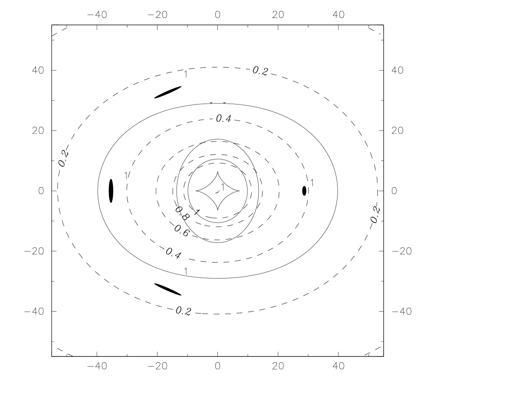
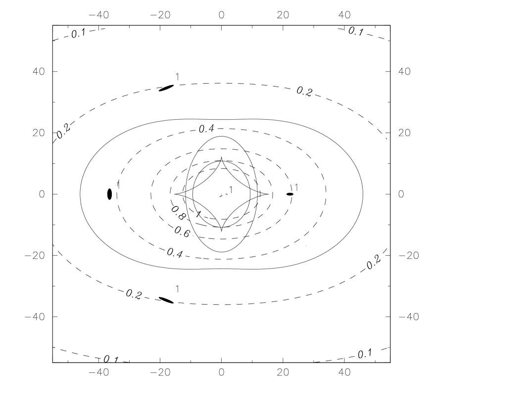
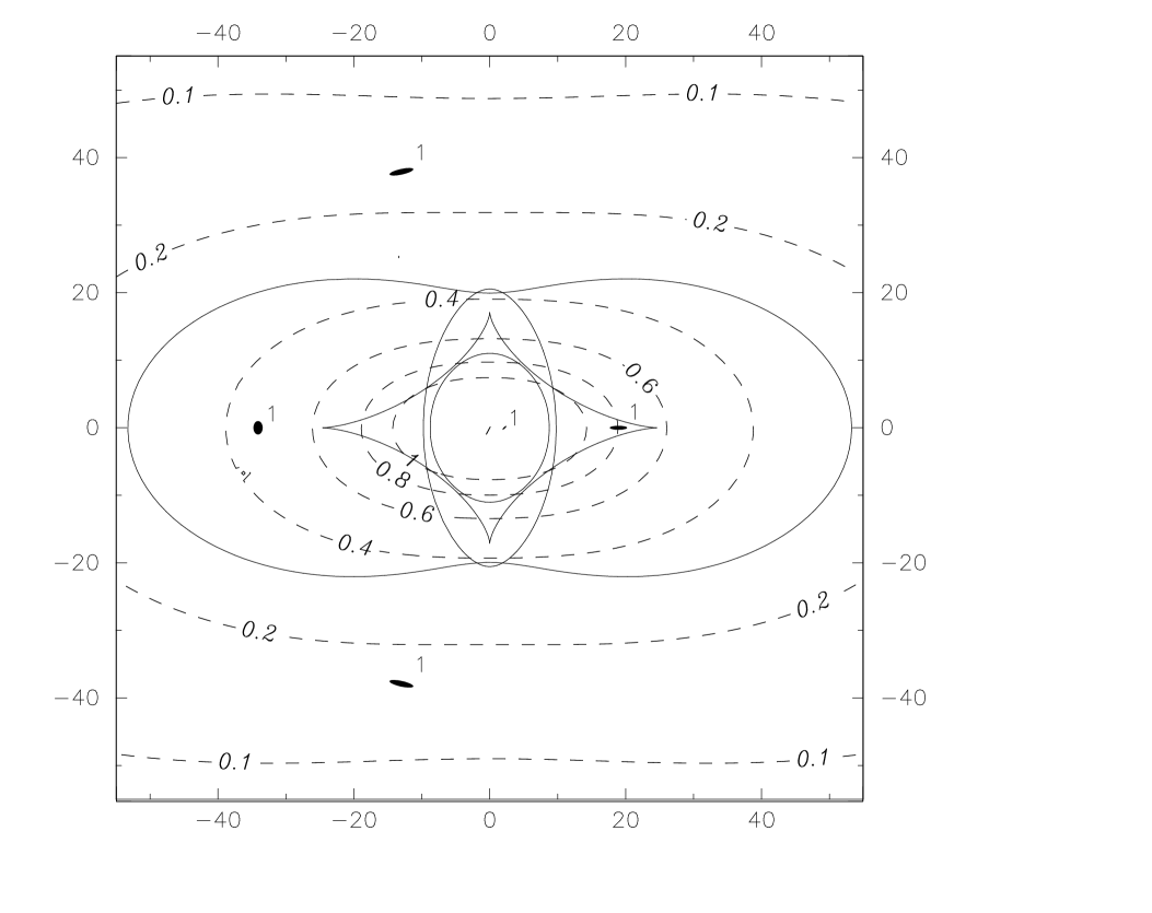
Figure 1: System of 5 multiple images generated by a pseudo-elliptical NFW cluster at $z_{L}=0.3$ with the following lens parameters: $v_{c}=2000$ km/s, $\theta_{s}=31.3$″($r_{s}=150$ kpc) and different values of $\epsilon$. From left to right : $\epsilon=0.1,\ 0.2,\ 0.3$. Solid lines are the critical and caustic lines for a source redshift $z_{S1}=1$. Dashed lines are the iso-contours of the dimensionless projected density $\displaystyle{\frac{\Sigma_{\epsilon}(x_{1}/r_{s},x_{2}/r_{s})}{2\rho_{c}r_{s}}}$. Units are given in arcseconds.

3 Elliptical Potential and Deflection-Angle Model

We will here introduce an ellipticity $\epsilon$ in the circular lens potential $\varphi(\theta)$. Moreover, we assume that the radial profile can be scaled by a scale radius $\theta_{s}$, thus making possible to define $x$ as $x=\theta/\theta_{s}$ (one can always set $\theta_{s}=1$ if the radial profile is scale free). We introduce the ellipticity in the expression of the lens potential by substituting $x$ by $x_{\varepsilon}$, using the following elliptical coordinate system:

$$\left\{\begin{array}[]{lcl}x_{1\epsilon}&=&\sqrt{a_{1\epsilon}}\,x_{1}\\ x_{2\epsilon}&=&\sqrt{a_{2\epsilon}}\,x_{2}\\ x_{\epsilon}&=&\sqrt{x_{1\epsilon}^{2}+x_{2\epsilon}^{2}}\ =\ \sqrt{a_{1\epsilon}x_{1}^{2}+a_{2\epsilon}x_{2}^{2}}\\ \phi_{\epsilon}&=&\arctan\left(x_{2\epsilon}/x_{1\epsilon}\right)\end{array}\right.$$ (12)

where $a_{1\epsilon}$ and $a_{2\epsilon}$ are two parameters defining the ellipticity.

Furthermore, from the elliptical lens potential $\varphi_{\epsilon}(x)\equiv\varphi(x_{\epsilon})$, we can then compute the elliptical deviation angle:

$$\@vec{\alpha}_{\epsilon}(\@vec{x})=\left(\begin{array}[]{l}\displaystyle{\frac{\partial\varphi_{\epsilon}}{\partial x_{1}}}=\alpha(x_{\epsilon})\sqrt{a_{1\epsilon}}\cos{\phi_{\epsilon}}\\ \displaystyle{\frac{\partial\varphi_{\epsilon}}{\partial x_{2}}}=\alpha(x_{\epsilon})\sqrt{a_{2\epsilon}}\sin{\phi_{\epsilon}}\\ \end{array}\right)$$ (13)

We note that these expressions holds for any definition of $a_{1\epsilon}$ and $a_{2\epsilon}$.

For instance, Meneghetti et al. (2002) use for their NFW elliptical model:

$$\begin{array}[]{ccl}a_{1\epsilon}&=&1-\epsilon\\ a_{2\epsilon}&=&1/(1-\epsilon)\end{array}$$ (14)

for an ellipticity along the $x_{1}$ axis. This choice has the advantage to stick to a ’standard’ definition: $\epsilon=1-b/a$ – where $a$ and $b$ are respectively the semi-major and semi-minor axis of the elliptical shape.

However this choice of $a_{1\epsilon}$ and $a_{2\epsilon}$ does not yield simple expressions for lensing quantities e.g. $\kappa$ and $\gamma$ (see Meneghetti et al., 2002)). Nevertheless, we will now show that it is possible to derive simple analytic expressions of $\kappa$ and $\gamma$ for a particular choice of $a_{1\epsilon}$ and $a_{2\epsilon}$.

At this point, our proposed method can be considered twofold. i) Either the circular lens potential $\varphi$ and the 2D surface mass density $\Sigma$ both have analytic expressions. We can then introduce the elliptical formalism (12) in the lensing potential $\varphi$ and derive the elliptical deflection angle $\@vec{\alpha}_{\epsilon}(\@vec{x})$ (Eq. (13)). ii) Or, there is no analytic expression for the circular lens potential (indeed, in many cases the circular lens potential has not a simple analytical expression). In this case, we need analytic expressions for both the circular deviation angle $\@vec{\alpha}$ and the 2D surface mass density $\Sigma$. The elliptical formalism (12) is then introduced in the expression of the deflection angle as in Eq. (13). The way the deviation angle is defined ensures that $\@vec{\alpha}(\@vec{x})$ derives from a lens potential $\varphi_{\epsilon}(x)\equiv\varphi(x_{\epsilon})$, even if there is no analytical expression for $\varphi(x)$.

Thus, in the following, we will refer to this method as the elliptical deflection angle model, whether the lens potential is analytically known or not. To be able to simply derive the convergence and the shear, we choose the following elliptical parameters:

$$\begin{array}[]{c}a_{1\epsilon}=1-\epsilon\\ a_{2\epsilon}=1+\epsilon\end{array}$$ (15)

For small $\epsilon$, it gives the same ellipticity along the $x_{1}$ axis as the one given by the parameters defined in Eqs (14). More generally, if we denote by $\epsilon_{\varphi}$ the ellipticity of the lens potential contours – taken as $1-b/a$ –, we have:

$$\epsilon_{\varphi}=1-\displaystyle{\sqrt{\frac{1-\epsilon}{1+\epsilon}}}$$ (16)

independently of the profile. This means there is a direct relation between the ’standard’ ellipticity and the deflection angle ellipticity.

However, for this particular choice of $\epsilon$ we can derive easily – using Eqs (7) – the corresponding convergence $\kappa_{\epsilon}(\@vec{x})$ induced by Eq. (13):

$$\kappa_{\epsilon}(\@vec{x}) = \displaystyle{\frac{1}{2\theta_{s}^{2}}\left(\frac{\partial^{2}\varphi_{\epsilon}}{\partial x_{1}^{2}}+\frac{\partial^{2}\varphi_{\epsilon}}{\partial x_{2}^{2}}\right)}$$ (17)

$$= \displaystyle{\kappa(\@vec{x}_{\epsilon})+\frac{\epsilon}{2\theta_{s}^{2}}\left(\frac{\partial^{2}\varphi(x_{\epsilon})}{\partial x_{2\epsilon}^{2}}-\frac{\partial^{2}\varphi(x_{\epsilon})}{\partial x_{1\epsilon}^{2}}\right)}$$

$$= \displaystyle{\kappa(\@vec{x}_{\epsilon})+\epsilon\cos{2\phi_{\epsilon}}\,\gamma(\@vec{x}_{\epsilon})}.$$

Similarly, the shear $\gamma_{\epsilon}(\@vec{x})$ can be written as:

$$\begin{array}[]{rl}\gamma_{\epsilon}^{2}(\@vec{x})&=\displaystyle{\frac{1}{4\theta_{s}^{4}}\left\{\left(\frac{\partial^{2}\varphi_{\epsilon}}{\partial x_{1}^{2}}-\frac{\partial^{2}\varphi_{\epsilon}}{\partial x_{2}^{2}}\right)^{2}+\left(2\frac{\partial^{2}\varphi_{\epsilon}}{\partial x_{1}\partial x_{2}}\right)^{2}\right\}}\\ &=\gamma^{2}(\@vec{x}_{\epsilon})\\ +\displaystyle{\frac{\epsilon}{2\theta_{s}^{4}}}&\displaystyle{\left(\frac{\partial^{2}\varphi(x_{\epsilon})}{\partial x_{2\epsilon}^{2}}-\frac{\partial^{2}\varphi(x_{\epsilon})}{\partial x_{1\epsilon}^{2}}\right)\left(\frac{\partial^{2}\varphi(x_{\epsilon})}{\partial x_{1\epsilon}^{2}}+\frac{\partial^{2}\varphi(x_{\epsilon})}{\partial x_{2\epsilon}^{2}}\right)}\\ +\displaystyle{\frac{\epsilon^{2}}{4\theta_{s}^{4}}}&\displaystyle{\left\{\left(\frac{\partial^{2}\varphi(x_{\epsilon})}{\partial x_{1\epsilon}^{2}}+\frac{\partial^{2}\varphi(x_{\epsilon})}{\partial x_{2\epsilon}^{2}}\right)^{2}-4\left(\frac{\partial^{2}\varphi(x_{\epsilon})}{\partial x_{1\epsilon}\partial x_{2\epsilon}}\right)^{2}\right\}}\end{array}$$ (18)

which, using Eqs (7), can be simplified as:

$$\gamma_{\epsilon}^{2}(\@vec{x})=\gamma^{2}(\@vec{x}_{\epsilon}) + 2\epsilon\cos{2\phi_{\epsilon}}\gamma(\@vec{x}_{\epsilon})\kappa(\@vec{x}_{\epsilon})$$ (19)

$$+ \epsilon^{2}(\kappa^{2}(\@vec{x}_{\epsilon})-\cos^{2}{2\phi_{\epsilon}}\gamma^{2}(\@vec{x}_{\epsilon})).$$

Finally, the projected mass density $\Sigma_{\epsilon}(\@vec{x})$ is simply determined from equations (17) and (6):

$$\Sigma_{\epsilon}(\@vec{x})=\Sigma(\@vec{x}_{\epsilon})+\epsilon\cos{2\phi_{\epsilon}}(\overline{\Sigma}(\@vec{x}_{\epsilon})-\Sigma(\@vec{x}_{\epsilon})).$$ (20)

4 Application of the Model to NFW Halos

Now, we apply the elliptical deflection angle model developed in Sect. 3 to the NFW profile (1). In that case, the lens potential (2) and the 2D projected mass profile (4) are known analytically.

An illustration of some lensed images using our new formalism applied to the NFW profile is shown in Fig. 1. The caustic associated with the tangential critical line has the usual diamond shape and is not reduced to a central point as in the spherical NFW case. This of course makes the formation of 5-image configurations with tangential images possible.

Figure 2: Ellipticity $\epsilon_{\Sigma}$ of the projected density $\Sigma_{\epsilon}$ as a function of the ellipticity $\epsilon$ defined in Eq.(12) with the choice (15) for the NFW profile. We show curves for different values of $r/r_{s}$ ($r$: ellipse semi diagonal, $r_{s}$: NFW scale radius).

Figure 3: Parameter $\epsilon_{\Sigma 2}$ from Eq. (24) used to fit the projected density $\Sigma_{\epsilon}$; it characterises the deviation from a purely elliptical curve. $\epsilon_{\Sigma 2}$ is a function of the ellipticity $\epsilon$ defined in Eq.(12) with the choice (15) for the NFW profile. Curves are shown for different values of $r/r_{s}$ ($r$: ellipse semi diagonal, $r_{s}$: NFW scale radius).

4.1 Expression of the 3D pseudo-elliptical mass distribution

This particular mass distribution has the advantage that the 3D pseudo-elliptical NFW mass profile $\rho_{\epsilon}(\@vec{x},x_{3})$ can also be derived. Indeed using the scaled variables $x_{3}=z/r_{s}$ and $u=r/r_{s}=\sqrt{x^{2}+x_{3}^{2}}$, we can compute from equations (4), (5) and (20):

$$\rho_{\epsilon}(\@vec{x},x_{3}) = \rho(\@vec{x}_{\epsilon},x_{3})$$ (21)

$$+ \epsilon\cos{2\phi_{\epsilon}}\left(\frac{2}{x_{\epsilon}^{2}}\int_{0}^{x_{\epsilon}}x\rho(\@vec{x},x_{3})dx-\rho(\@vec{x}_{\epsilon},x_{3})\right)$$

$$= \rho(\@vec{x}_{\epsilon},x_{3})$$

$$+ \epsilon\cos{2\phi_{\epsilon}}\left(\overline{\rho}(\@vec{x}_{\epsilon},x_{3})-\rho(\@vec{x}_{\epsilon},x_{3})\right)$$

with

$$\overline{\rho}\left(\sqrt{u^{2}-x_{3}^{2}},x_{3}\right)=\frac{2\rho_{c}}{(1+u)(1+x_{3})(u+x_{3})}$$ (22)

4.2 Physical limits of the NFW pseudo-elliptical mass model

We now investigate the range of $\epsilon$ for which this NFW mass model is an adequate description of an elliptical underlying mass distribution. We will use two methods to quantify the deviation of our model from a purely elliptical distribution.

Fig. 1 shows the contours (dashed lines) of the projected mass density $\Sigma_{\epsilon}$ (Eq. (20)) for $\epsilon=0.1,0.2,0.3$. In the more elliptical models, the contours become increasingly boxy/peanut shaped at larger “radius”. In order to investigate this boxy behaviour, we must first quantify the ellipticity $\epsilon_{\Sigma}$ of the projected mass distribution $\Sigma_{\epsilon}$, and then relate this to the ellipticity $\epsilon$ of the lens model. Purely elliptical projected mass density contours would have a polar equation of the type

$$r\propto\displaystyle{\frac{1}{\sqrt{(1-\epsilon_{\Sigma})\cos^{2}\phi+\displaystyle{\frac{\sin^{2}\phi}{1-\epsilon_{\Sigma}}}}}}.$$ (23)

We propose a fit of elliptical-like functions which is a deviation from an elliptical model. It is slightly different from the function presented by Jedrzejewski (1987) and already used by Shaw (1993) or Quillen et al. (1997). We write the polar equation

$$r\propto\displaystyle{\frac{1}{\sqrt{(1-\epsilon_{\Sigma})\cos^{2}\phi+\displaystyle{\frac{\sin^{2}\phi}{1-\epsilon_{\Sigma}}}+\epsilon_{\Sigma 2}\cos(4\phi_{\epsilon_{\Sigma}})}}}$$ (24)

with

$$\phi_{\epsilon_{\Sigma}}=\arctan\left(\displaystyle{\frac{\tan\phi}{1-\epsilon_{\Sigma}}}\right).$$ (25)

If we assume that the fitted contour is roughly an ellipse with an ellipticity $\epsilon_{\Sigma}$, the angular direction $\phi_{ab}$ of its diagonal is such that $\tan\phi_{ab}=b/a\simeq 1-\epsilon_{\Sigma}$. In this expression, $a$ and $b$ are defined by $\Sigma_{\epsilon}(a,0)=\Sigma_{\epsilon}(0,b)$, i.e. the “pseudo” semi major and minor axis. Taking a radial coordinate of the form (24) permits to quantify the degree of boxiness for a non elliptical model. Indeed, compared to an ellipse, $r$ is then smaller along the axis and larger along the diagonals for $\epsilon_{\Sigma 2}>0$, i.e. the distribution is boxier. This kind of fit can be generally applied to check quantitatively the deviation of a boxy/peanut function from an ellipse via the parameter $\epsilon_{\Sigma 2}$.

Figure 4: Solid lines: projected density $\Sigma_{\epsilon}(x_{1}/r_{s},x_{2}/r_{s})$ contour for a pseudo-elliptical NFW profile at $r/r_{s}=10$ ($r$: ellipse semi diagonal, $r_{s}$: NFW scale radius). Dotted lines: best fit ellipse. Dashed lines: fitting function (24) with computed parameters $\epsilon_{\Sigma}$ and $\epsilon_{\Sigma 2}$. From left to right: $\epsilon=0.1,0.2,0.3$.

Figure 5: Goodness of fit of the projected density $\Sigma_{\epsilon}$ contours by a function of the type (24). The ellipticity $\epsilon$ is defined for the NFW profile in Eq.(12) with the choice (15). Curves are shown for different values of $r/r_{s}$ ($r$: ellipse semi diagonal, $r_{s}$: NFW scale radius).The goodness of fit is computed as in Eq. (27) with $N=20$.

For a given ellipticity $\epsilon$, introduced in the deflection angle, and a given radius $r=\sqrt{a^{2}+b^{2}}$, we will fit the parameters $\epsilon_{\Sigma}$ and $\epsilon_{\Sigma 2}$ in the corresponding surface density profile. A goodness of fit indicator will allow us to check how effective the representation is. The ratio $b/a$ gives a first relation. The other one is given by $c/a$ where $c$ is such that $\Sigma_{\epsilon}(c,c\tan\phi_{ab})=\Sigma_{\epsilon}(a,0)=\Sigma_{\epsilon}(0,b)$. This means that we adjust the coefficients of the fitting function along the first order ellipse diagonal. Eq. (24) is indeed a deviation from an ellipse in this direction. Actually, getting two relations does not lead analytically to $\epsilon_{\Sigma}$ and $\epsilon_{\Sigma 2}$, mainly because of the angle $\phi_{\epsilon_{\Sigma}}$ which depends on $\epsilon_{\Sigma}$. So we assume in practice that $1-\epsilon_{\Sigma}\simeq b/a$. This approximation is correct since

$$\frac{b}{a}=\displaystyle{\frac{\sqrt{1-\epsilon_{\Sigma}+\epsilon_{\Sigma 2}}}{\sqrt{\displaystyle{\frac{1}{1-\epsilon_{\Sigma}}}+\epsilon_{\Sigma 2}}}}\simeq(1-\epsilon_{\Sigma})\left(1+\frac{\epsilon_{\Sigma}\epsilon_{\Sigma 2}}{2}\left(\frac{2-\epsilon_{\Sigma}}{1-\epsilon_{\Sigma}}\right)\right)$$ (26)

for $\epsilon_{\Sigma 2}\ll 1$ and $1-\epsilon_{\Sigma}=O(1)$. It is then possible to express $\epsilon_{\Sigma}$ and $\epsilon_{\Sigma 2}$ analytically for given $\epsilon$ and $r$, see Figs (2) and (3).

We note that a given value of $\epsilon$ corresponds to a higher value of $\epsilon_{\Sigma}$ (Fig. (2)). $\epsilon$ can be considered as the ellipticity of the potential $\epsilon_{\varphi}$ for a large range of values (see Eq. (16): there is less than 10% error for $\epsilon\leq 0.25$). It is also known that the ellipticity of the projected mass density is proportional to and larger than the ellipticity of the potential in the linear approximation and then flattens (Kneib, 1993). For instance, a singular isothermal ellipse satisfies $\epsilon_{\Sigma}=3\,\epsilon_{\varphi}$ for $\epsilon_{\varphi}\ll 1$.

To derive numerically such a relation for the NFW profile, we need to know the range of acceptable and physical values for $\epsilon$. For all ellipticities and up to $r/r_{s}=10$ (i.e. $r\sim 1.5$ Mpc for a galaxy cluster), $\epsilon_{\Sigma 2}<0.1$ (see Fig. (3)). So the deviation parameter is not too large and the elliptical approximation could be considered as acceptable if the goodness of fit for the function (24) is small. To check the relevance of this fit, we plot the $\Sigma_{\epsilon}$ contour, the first order ellipse and the fitting function found for $r/r_{s}=10$ and $\epsilon=0.1,0.2,0.3$ (Fig. (4)). The fit is correct for small ellipticities but is not suited for $\epsilon=0.3$. In particular it fails to reproduce the shape along the $x_{2}$ axis.

Quantitatively, we define a goodness of fit in the following way:

$$gof=\frac{1}{N}\sum_{i=1}^{N}\frac{|r_{\Sigma}(\phi_{i})-r(\phi_{i})|}{r(\phi_{i})}.$$ (27)

for $\phi_{i}=\displaystyle{\frac{\pi}{2}\frac{i}{N}}$ (for symmetry reasons). For given $a$ and $\epsilon$, $r_{\Sigma}(\phi_{i})$ and $r(\phi_{i})$ are respectively the distances of the projected density contour and of the corresponding fit function (24) from the centre in the direction $\phi_{i}$. Fig. (5) confirms that the goodness of fit becomes quite large from $\epsilon\sim 0.25$ (the deviation from the proposed function then reaches 10%).

We think that function (24) can be useful to test deviation from ellipticity of a given function in various sets of problems. In our case the deviation parameter $\epsilon_{\Sigma 2}$ is rather small but the goodness of fit is only acceptable for ellipticities (introduced in the deviation angle) of $\epsilon<0.25$.

Alternatively, to simply quantify the degree of boxiness for this pseudo-elliptical NFW model, we defined the characteristic deviation from ellipticity in the following way. On Fig. 6, $\delta r$ is the distance between a real ellipse and a $\Sigma_{\epsilon}$ contour along the ellipse diagonal. We plot $\delta r/r$ versus $\epsilon$ for different $r/r_{s}$ ratios in Fig. 7. At all radii, and for all $\epsilon$, the model has a positive $\delta r$, i.e. the model mass distribution is more boxy than an elliptical distribution. Assuming that the underlying mass distribution is elliptical, and aiming to incur an error in $r$ which is $\lesssim 10$%, we find that on scales of 1.5 Mpc (i.e. corresponding to $r/r_{s}\sim 10$ for a galaxy cluster), the pseudo-elliptical model provides an adequate description of the underlying mass distribution for $\epsilon\lesssim 0.25$, which translates to a limit of $\epsilon_{\Sigma}\lesssim 0.4$ on the projected density at $r/r_{s}=1$ (see Fig. 2).

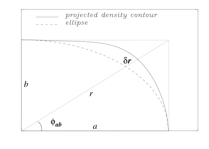
Figure 6: Method used to compare a projected density contour and a real ellipse with semi axes $a$ and $b$. $\delta r/r$ characterises this deviation.

Figure 7: $\delta r/r$ (as defined in Fig. 6) as a function of $\epsilon$. It characterises the deviation of the projected density from an ellipsoidal model for various $r/r_{s}$ ratios ($r_{s}$: NFW scale radius).

Figure 8: $b/r_{s}$ ($b$: distance from the centre along the $x_{2}$ axis at which $\Sigma_{\epsilon}$ becomes negative, $r_{s}$: NFW scale radius) as a function of $\epsilon$.

For models in which the potential – rather than the deflection angle – is chosen to have elliptical contours, the corresponding density contours acquire the artificial feature of a dumbbell shape, and the density can also become negative (Kassiola & Kovner, 1993). Similarly here, for large ellipticities or at large radii, we see from Eq.(20) that the projected density $\Sigma_{\epsilon}$ can also become negative. This occurs closer to the centre along the $x_{2}$ axis where $\cos{2\phi_{\epsilon}}=-1$. For each value of the ellipticity $\epsilon$, we plot in Fig. 8 the scaled distance $b/r_{s}$ at which $\Sigma_{\epsilon}(0,b)$ becomes negative. If we decide to have physical (i.e. positive) mass density up a scale of 1.5 Mpc (typically $b/r_{s}=10$ for a cluster), we have to restrict ourselves to ellipticities smaller than $\epsilon\sim 0.3$ (i.e. $\epsilon_{\Sigma}\sim 0.6$ at $r/r_{s}=1$ from Fig. 2). So a relatively broad range of systems can be modelled in a physically consistent way.

We want to obtain an explicit, if approximate, relationship between the ellipticity $\epsilon$ introduced in the deviation angle and the ellipticity of the projected mass density $\epsilon_{\Sigma}$ it induces. In the acceptable and physical range $[0,0.25]$ for $\epsilon$, we fit a polynomial of the form:

$$\epsilon_{\Sigma}=a_{1}\,\epsilon+a_{2}\,\epsilon^{2}.$$ (28)

A fit for $r=r_{s}$ leads to $\epsilon_{\Sigma}=2.27\,\epsilon-2.03\,\epsilon^{2}$ with a $\chi^{2}=3.9\,10^{-7}$. More generally, the coefficients $a_{i}$ depend on $x=r/r_{s}$. A fit between $x=0$ and $x=10$ gives

$$\left\{\begin{array}[]{ccrcc}a_{1}&=&2.12&+&0.179\,x\\ a_{2}&=&-1.70&-&0.328\,x\end{array}\right.$$ (29)

with a $\chi^{2}=2.9\,10^{-3}$.

In summary, we can say that the deviation angle elliptical model can be applied to NFW mass profile up to $\epsilon\sim 0.25$. For this range of values, $\epsilon$ can be identified with the ellipticity of the potential $\epsilon_{\varphi}$, and the ellipticity of the projected mass density $\epsilon_{\Sigma}$ is about twice larger than $\epsilon$.

5 Conclusion

We propose a simple new formalism that introduces the ellipticity into the lens potential/deflection-angle of a circular mass model. The method can be applied when the lens potential or/and the deviation angle takes an analytical form. Then for radial mass profiles for which the 2D surface density $\Sigma$ also has an analytical expression, this formalism gives analytical expressions of a pseudo-elliptical mass distribution for the deviation angle, the projected mass density, the convergence and shear.

Whatever the form of the mass distribution, the elliptical parameter $\epsilon$ is simply expressed as a function of the ellipticity of the potential. This is particularly helpful in getting some insight on the physical meaning of this parameter.

We have applied this formalism to the NFW profile and estimated the range of ellipticity ($\epsilon\lesssim 0.25$, or $\epsilon_{\Sigma}\lesssim 0.4$) for which this model is a good description of elliptical mass distributions and thus can be reliably applied to observational data. To derive these limits, we introduced a particular fit for elliptical-like profiles, that can be useful in similar cases.

Our proposed method is particularly useful when it is essential to quickly calculate the potential, the deflection angle and magnification of many images and/or many mass clumps. This is particularly important when using inverse methods (such as maximum likelihood) to investigate galaxy-galaxy lensing in the field or in clusters of galaxies, or to compute time delays.

References

• Barkana (1998) Barkana, R. 1998, ApJ, 502, 531
• Bartelmann (1996) Bartelmann, M. 1996, A&A, 313, 697
• Faber et al. (1997) Faber, S. M., Tremaine, S., Ajhar, E. A., et al. 1997, AJ, 114, 1771
• Ghigna et al. (2000) Ghigna, S., Moore, B., Governato, F., et al. 2000, ApJ, 544, 616
• Golse et al. (2002) Golse, G., Kneib, J.-P., & Soucail, G. 2002, A&A, 387, 788
• Hjorth & Kneib (2002) Hjorth, J. & Kneib, J.-P. 2002, ApJ, submitted
• Jedrzejewski (1987) Jedrzejewski, R. I. 1987, MNRAS, 226, 747
• Kassiola & Kovner (1993) Kassiola, A. & Kovner, I. 1993, ApJ, 417, 450
• Kneib (1993) Kneib, J.-P. 1993, PhD thesis, Université Paul-Sabatier, Toulouse
• Kneib (2001) Kneib, J.-P. 2001, in Yale 2001 Cosmology Workshop on the Shapes of Galaxies and Their Halos, astro-ph/0112123
• Meneghetti et al. (2002) Meneghetti, M., Bartelmann, M., & Moscardini, L. 2002, MNRAS, submitted, astro-ph/0201501
• Miralda-Escudé (1991) Miralda-Escudé, J. 1991, ApJ, 370, 1
• Moore et al. (1998) Moore, B., Governato, F., Quinn, T., et al. 1998, ApJ, 499, L5
• Muñoz et al. (2001) Muñoz, J. A., Kochanek, C. S., & Keeton, C. R. 2001, ApJ, 558, 657
• Navarro et al. (1997) Navarro, J. F., Frenk, C. S., & White, S. D. M. 1997, ApJ, 490, 493
• Quillen et al. (1997) Quillen, A., Kuchinski, L., Frogel, J., & DePoy, D. 1997, ApJ, 481, 179
• Schneider et al. (1992) Schneider, P., Ehlers, J., & Falco, E. E. 1992, Gravitational Lensing (Springer-Verlag)
• Shaw (1993) Shaw, M. 1993, MNRAS, 261, 718
• Smith et al. (2001) Smith, G. P., Kneib, J.-P., Ebeling, H., et al. 2001, ApJ, 552, 493
• Wright & Brainerd (2000) Wright, C. O. & Brainerd, T. G. 2000, ApJ, 534, 34