Strong Gravitational Lensing Time Delay Statistics
and the Density Profile of Dark Halos

Abstract

The distribution of differential time delays $\Delta t$ between images produced by strong gravitational lensing contains information on the mass distributions in the lensing objects as well as on cosmological parameters such as $H_{0}$. We derive an explicit expression for the conditional probability distribution function of time delays $P(\Delta t\,|\,\theta)$, given an image separation between multiple images $\theta$, and related statistics. We consider lensing halos described by the singular isothermal sphere (SIS) approximation and by its generalization as proposed by Navarro, Frenk, & White (NFW) which has a density profile $\rho\propto r^{-\alpha}$ in the innermost region. The time delay distribution is very sensitive to these profiles; steeper inner slopes tend to produce larger time delays. For example, if $H_{0}=70\,{\rm km\,s^{-1}Mpc^{-1}}$, a $\Lambda$-dominated cosmology and a source redshift $z_{\rm S}=1.27$ are assumed, lenses with $\theta=5^{{}^{\prime\prime}}$ produce a time delay of $\Delta t[{\rm yr}]=1.5^{+1.7}_{-0.9}$, $0.39^{+0.37}_{-0.22}$, $0.15^{+0.11}_{-0.09}$, and $0.071^{+0.054}_{-0.038}$ (50% confidence interval), for SIS, generalized NFW with $\alpha=1.5$, $\alpha=1.0$, and $\alpha=0.5$, respectively. At a fixed image separation, the time delay is determined by the difference in the lensing potential between the position of the two images, which typically occur at different impact parameters. Although the values of $\Delta t$ are proportional to the inverse of $H_{0}$, $P(\Delta t\,|\,\theta)$ is rather insensitive to all other cosmological model parameters, source redshifts, magnification biases and so on. A knowledge of $P(\Delta t\,|\,\theta)$ will also be useful in designing the observing program of future large scale synoptic variability surveys and for evaluating possible selection biases operating against large splitting lens systems.

1 Introduction

The cold dark matter (CDM) scenario predicts relatively cuspy dark matter halos. On the basis of systematic N-body simulations, Navarro, Frenk, & White (1996, 1997, hereafter NFW) found that the density profile obeys the “universal” form $\rho(r)\propto r^{-1}(r+r_{\rm s})^{-2}$ irrespective of the underlying cosmological parameters, the shape of the primordial fluctuation spectrum and the formation histories. Recent high resolution simulations suggest even steeper cusps $\rho\propto r^{-1.5}$ in the innermost region (Moore et al., 1999; Fukushige & Makino, 2001a, b), and a weak dependence of the inner slope on the halo mass is also reported (Jing & Suto, 2000).

The statistics of strong gravitational lensing have been used to probe the density profiles of dark halos, e.g., multiple QSO images (Fox & Pen, 2001; Keeton & Madau, 2001; Wyithe, Turner, & Spergel, 2001; Li & Ostriker, 2001; Takahashi & Chiba, 2001) and the long thin arcs (Williams, Navarro, & Bartelmann, 1999; Meneghetti et al., 2001; Molikawa & Hattori, 2001; Oguri, Taruya, & Suto, 2001). These theoretical studies concluded that gravitational lensing rates are extremely sensitive to the inner slope of dark halos. The lensing statistics of small separations, however, will also be affected by gas cooling and clumpiness in the host halo (Keeton, 1998; Porciani & Madau, 2000; Kochanek & White, 2001; Li & Ostriker, 2001). Thus multiple QSO images with intermediate or large separations, $\theta\gtrsim 5^{{}^{\prime\prime}}$, are more relevant in constraining the density profile of “pure” dark halos.

At present, several lensing surveys at large separations have been carried out; e.g., the Jodrell-Bank VLA Astrometric Survey and the Cosmic Lens All Sky Survey (JVAS/CLASS; e.g., Browne & Myers, 2001) and Arcminute Radio Cluster-lens Search (ARCS; e.g., Phillips, Browne, & Wilkinson, 2001). The JVAS/CLASS sample comprises 10,499 radio sources. An explicit search for lenses has detected no lenses with image separations $6^{{}^{\prime\prime}}<\theta<15^{{}^{\prime\prime}}$ (Phillips et al., 2000), while 18 gravitational lenses with $0.3^{{}^{\prime\prime}}<\theta<3^{{}^{\prime\prime}}$ were found (Helbig, 2000). ARCS also produced a null result for lensing events with $15^{{}^{\prime\prime}}<\theta<60^{{}^{\prime\prime}}$ from 1,023 extended radio sources. The lack of large separation images is only marginally consistent if the usual NFW profile and $\Lambda$-dominated CDM model are assumed (Li & Ostriker, 2001; Keeton & Madau, 2001), but it also may be ascribed in part to an effect of the longer time delays between more widely separated images. Any intrinsic variability of the QSO will result in images which less resemble each other for longer delays (Phillips et al., 2001).

So far, time delays between two images have been used primarily to estimate the Hubble constant $H_{0}$ using a detailed lens model of each system (e.g., Grogin & Narayan, 1996; Barkana et al., 1999). But the importance of mass distribution in estimating Hubble constant has been recognized (Impey et al., 1998; Keeton et al., 2000; Witt, Mao, & Keeton, 2000) and this led to an attempt to constrain the galaxy mass profile from time delays using Monte Carlo simulations (Rusin, 2000). Instead, in this paper, we consider the statistics of the time delay effect analytically. We derive an expression for the cumulative joint probability, i.e., the probability that the time delay is larger than $\Delta t$ and the image separation is $\theta$, $P(>\!\Delta t,\theta)$, and also various related statistics. They allow us to estimate the range of probable time delays for a given image separation and the extent to which the intrinsic time variability of quasars affects observed strong gravitational lensing rates. Our most important result is that the distribution of delays is quite sensitive to the density profiles of the lensing objects. For example, an NFW density profile predicts median time delays a factor of three or so smaller than the density profile proposed by Moore et al. (1999) and Fukushige & Makino (2001a, b) for the same $H_{0}$ value. While the lenses for which time delays are currently observed are dominated by barionic component, we can constrain the density profile of dark halos if a sample of time delays with large separations becomes available. It turns out that the time delay statistics are fairly insensitive to other uncertainties, such as the magnification bias and various cosmological parameters and therefore become a relatively reliable estimator for the density profile of dark halos.

Of course, all delay values are linearly proportional to the inverse Hubble constant, and we here assume its value to be $H_{0}=70\,{\rm km\,s^{-1}Mpc^{-1}}$, which is consistent with the final result of Hubble Space Telescope Key Project (Freedman et al., 2001), throughout the remainder of our discussion.

The outline of this paper is as follows. In §2, we briefly describe the usual formulation of gravitational lensing statistics. Section 3 presents the analytic formulation of time delay statistics. Our main results are shown in §4. Finally we summarize the main results and discuss their application in §5.

2 Description of Gravitational Lensing Statistics

2.1 Basic Equations

We denote the image position in the lens plane by $\vec{\xi}$ and the source position in the source plane by $\vec{\eta}$. We assume spherically symmetric lens objects throughout the paper. In this case, the lens equation (e.g., Schneider, Ehlers, & Falco, 1992) reduces to

$$y=x-\beta(x),$$ (1)

where $x=|\vec{\xi}|/\xi_{0}$, $y=|\vec{\eta}|D_{\rm OL}/\xi_{0}D_{\rm OS}$, $\xi_{0}$ is the characteristic length in the lens plane (see §2.3.), and $D_{\rm OL}$ and $D_{\rm OS}$ denote the angular diameter distances from the observer to the lens and the source planes, respectively. The explicit expressions of the scaled deflection angles $\beta(x)$ for the specific lens models are presented in §2.3.

We consider a halo of mass $M$ in the lens plane at a redshift $z_{\rm L}$ and a source located at $z_{\rm S}$. Then the gravitational lensing cross section $\sigma(>\!\theta,>\!\mu)$, defined in the lens plane, for multiple images with image separation larger than $\theta$ and magnification larger than $\mu$ is given by

$$\sigma(>\!\theta,>\!\mu)=\pi\,y_{\rm r}^{2}\,\xi_{0}^{2}\,\Theta(\theta(M,z_{\rm S},z_{\rm L})-\theta)\,p(>\!\mu),$$ (2)

where $y_{\rm r}$ is the critical source position to form multiple images (usually given by the position of the radial caustic), $\Theta(x)$ is the Heaviside step function, and $p(>\!\mu)$ denotes the fraction of area satisfying $>\!\mu$:

$$p(>\!\mu)=\frac{2}{y_{\rm r}^{2}}\int_{0}^{y_{\rm r}}dy\,y\,\Theta(\mu(y)-\mu).$$ (3)

From this cross section, the probability that a source at $z_{\rm S}$ is multiply lensed with image separation larger than $\theta$ and magnification larger than $\mu$ is

$$P(>\!\theta,>\!\mu;z_{\rm S})=\int_{0}^{z_{\rm S}}dz_{\rm L}\int_{M_{\rm min}}^{\infty}dM\,\pi\,y_{\rm r}^{2}\,\xi_{0}^{2}\,p(>\!\mu)\frac{c\,dt}{dz_{\rm L}}(1+z_{\rm L})^{3}n(M,z_{\rm L}),$$ (4)

where $M_{\rm min}$ is determined by solving the equation; $\theta=\theta(M_{\rm min},z_{\rm S},z_{\rm L})$.

To calculate the lens mass distribution, we employ the Press-Schechter function (Press & Schechter, 1974):

$$n_{\rm PS}(M,z)=\sqrt{\frac{2}{\pi}}\frac{\rho_{0}}{M}\frac{\delta_{0}(z)}{\sigma_{M}^{2}}\left|\frac{d\sigma_{M}}{dM}\right|\exp\left[-\frac{\delta_{0}^{2}(z)}{2\sigma_{M}^{2}}\right],$$ (5)

where $\sigma_{M}$ is the rms of linear density fluctuation on mass scale $M$ at $z=0$ and $\delta_{0}(z)$ is the critical linear density contrast, $\delta_{0}(z)\sim 1.69/D(z)$, with $D(z)$ being the linear growth rate normalized to unity at $z=0$.

The corresponding differential probability with respect to the image separation is

$$P(\theta,>\!\mu;z_{\rm S}) \equiv -\frac{d}{d\theta}P(>\!\theta,>\!\mu;z_{\rm S})$$ (6)

$$= \int_{0}^{z_{\rm S}}dz_{\rm L}\,\frac{c\,dt}{dz_{\rm L}}(1+z_{\rm L})^{3}\left[\frac{dM}{d\theta}\pi\,y_{\rm r}^{2}\,\xi_{0}^{2}\,p(>\!\mu)n(M,z_{\rm L})\right]_{M=M_{\rm min}}.$$

2.2 Magnification Bias

So far, we have not considered magnification bias (Turner, 1980; Turner, Ostriker, & Gott, 1984). For a source of luminosity $L$, the effect of the magnification bias may be included as follows:

$$P^{\rm B}(\theta;z_{\rm S},L) = \frac{1}{\Phi(z_{\rm S},L)}\int_{1}^{\infty}d\mu\left|\frac{d}{d\mu}P(\theta,>\!\mu;z_{\rm S})\right|\Phi(z_{\rm S},L/\mu)\frac{1}{\mu}$$ (7)

$$= \int_{0}^{z_{\rm S}}dz_{\rm L}\,\frac{c\,dt}{dz_{\rm L}}(1+z_{\rm L})^{3}\left[\frac{dM}{d\theta}\pi\,y_{\rm r}^{2}\,\xi_{0}^{2}\,B(z_{\rm S},L)n(M,z_{\rm L})\right]_{M=M_{\rm min}},$$

where $\Phi(z_{\rm S},L)$ is the luminosity function of sources and $B(z_{\rm S},L)$ is

$$B(z_{\rm S},L)=\frac{2}{y_{\rm r}^{2}\Phi(z_{\rm S},L)}\int_{0}^{y_{\rm r}}dy\,y\,\Phi(z_{\rm S},L/\mu(y))\frac{1}{\mu(y)}.$$ (8)

Thus the probability distribution taking account of the magnification bias is simply expressed as equation (6) with $p(>\!\mu)$ replaced by $B(z_{\rm S},L)$. By neglecting magnification bias for simplicity, we may simply set $B(z_{\rm S},L)=1$.

It should be noted that $\mu(y)$ may be interpreted as the magnification of the total images, of the brighter, or of the fainter image among the outer two images, depending on the observational selection procedure for finding gravitational lens systems (Sasaki & Takahara, 1993; Cen et al., 1994). As indicated in §2.3.2, however, such a different choice of magnification does not affect the conditional time delay probability very much, especially for small inner slope values, while it changes the lensing rate by a factor of two. Thus we choose to designate the magnification $\mu(y)$ in the bias factor (eq. [8]) as the total magnification of all images throughout this paper.

2.3 Specific Density Profiles

2.3.1 Singular Isothermal Sphere

The SIS (Singular Isothermal Sphere) density profile is usually characterized by a one-dimensional velocity dispersion $v$:

$$\rho(r)=\frac{v^{2}}{2\pi Gr^{2}}.$$ (9)

In this case, we choose the characteristic length $\xi_{0}$ as

$$\xi_{0}=4\pi\left(\frac{v}{c}\right)^{2}\frac{D_{\rm OL}D_{\rm LS}}{D_{\rm OS}}.$$ (10)

Then the lens equation has two solutions $x_{\pm}=y\pm 1$ if $|y|\leq y_{\rm r}=1$. The separation between two image may be written as

$$\theta=\frac{\xi_{0}(x_{+}-x_{-})}{D_{\rm OL}}=8\pi\left(\frac{v}{c}\right)^{2}\frac{D_{\rm LS}}{D_{\rm OS}}.$$ (11)

The magnification of each image is

$$\mu_{\pm}(y)=\left|\frac{y}{x_{\pm}}\frac{dy}{dx_{\pm}}\right|^{-1}=\pm\frac{x_{\pm}}{y}=\frac{1}{y}\pm 1,$$ (12)

and their total magnification is given by

$$\mu(y)=\frac{2}{y}.$$ (13)

To compute the probability distribution functions (6) and (7), we also convert the mass function (eq. [5]) to a velocity function by using the spherical collapse model (e.g., Nakamura & Suto, 1997).

2.3.2 Generalized NFW Profile

The halo density profiles predicted by recent N-body simulations may be parameterized as a one-parameter family, the generalized NFW profile (Jing & Suto, 2000):

$$\rho(r)=\frac{\rho_{\rm crit}\delta_{\rm c}}{\left(r/r_{\rm s}\right)^{\alpha}\left(1+r/r_{\rm s}\right)^{3-\alpha}},$$ (14)

where $r_{\rm s}$ is a scale radius and $\delta_{\rm c}$ is a characteristic density. The profile with $\alpha=1$ corresponds that NFW originally proposed, while the profile with $\alpha=1.5$ resembles the one claimed by Moore et al. (1999) and Fukushige & Makino (2001a, b). The scale radius generally depends on the mass and the redshift, and is related to the concentration parameter:

$$c_{\rm vir}(M,z)\equiv\frac{r_{\rm vir}(M,z)}{r_{\rm s}(M,z)}.$$ (15)

The characteristic density is given by

$$\delta_{\rm c}=\frac{\Delta_{\rm vir}\Omega_{\rm vir}}{3}\frac{(3-\alpha)c_{\rm vir}^{\alpha}}{{}_{2}F_{1}\left(3-\alpha,3-\alpha;4-\alpha;-c_{\rm vir}\right)},$$ (16)

with ${}_{2}F_{1}\left(a,b;c;x\right)$ being the hypergeometric function (e.g., Keeton & Madau, 2001). Following Oguri et al. (2001), we adopt the mass and redshift dependence reported by Bullock et al. (2001) and consider the median amplitude of the concentration parameter $c_{\rm norm}$:

$$c_{\rm vir}(M,z)=c_{\rm norm}\frac{2-\alpha}{1+z}\left(\frac{M}{10^{14}h^{-1}M_{\odot}}\right)^{-0.13},$$ (17)

where $h$ denotes the Hubble constant in units of $100\,{\rm km\,s^{-1}Mpc^{-1}}$. Scatter of the concentration parameter is modeled by a log-normal function with the dispersion of $\sigma_{c}=0.18$ (Jing, 2000; Bullock et al., 2001). We fix $c_{\rm norm}$ to the value estimated in the simulations (Bullock et al., 2001), $c_{\rm norm}=8$, throughout this paper.

In these profiles, we choose $\xi_{0}=r_{\rm s}$ and denote the scaled deflection angle $\beta(x)$ as $\beta(x)=b\,f(x)$. The dimensionless factor $b$ (of order unity) and the function $f(x)$ are related to the dark halo profile as follows:

$$b=\frac{16\pi G\rho_{\rm crit}\delta_{\rm c}r_{\rm s}}{c^{2}}\frac{D_{\rm OL}D_{\rm LS}}{D_{\rm OS}},\\$$ (18)

$$f(x)=\frac{1}{x}\int_{0}^{\infty}dz\int_{0}^{x}dx^{\prime}\frac{x^{\prime}}{\left(\sqrt{x^{{}^{\prime}2}+z^{2}}\right)^{\alpha}\left(1+\sqrt{x^{{}^{\prime}2}+z^{2}}\right)^{3-\alpha}}.$$ (19)

The lens equation has three solutions $x_{1},x_{2},x_{3}\;(x_{1}>x_{2}>x_{3})$ if $|y|<y_{\rm r}$, where $y_{\rm r}$ is the position of the radial caustic. The image separation is defined between the outer two solution and is approximated as (Hinshaw & Krauss, 1987):

$$\theta\equiv\frac{\xi_{0}(x_{1}-x_{3})}{D_{\rm OL}}\simeq\frac{2r_{\rm s}x_{\rm t}}{D_{\rm OL}},$$ (20)

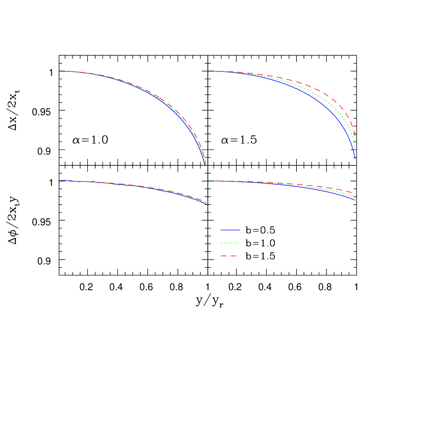
Figure 1: Accuracy of approximations for generalized NFW profiles with various parameters $b$ (eq. [18]) and the inner slope $\alpha$; $\alpha=1.0$ (left panels) and $\alpha=1.5$ (right panels). Upper panels display the ratio of the image separation and its approximation (eq. [20]). Lower panels give the ratio of the difference of the Fermat potential and its approximation (eq. [50]).

where $x_{\rm t}$ is the position of the tangential critical curve (the Einstein radius). The approximation (eq. [20]) is sufficiently accurate for the range of interest here (Upper panels of Figure 1), and is useful in computing the lensing probability.

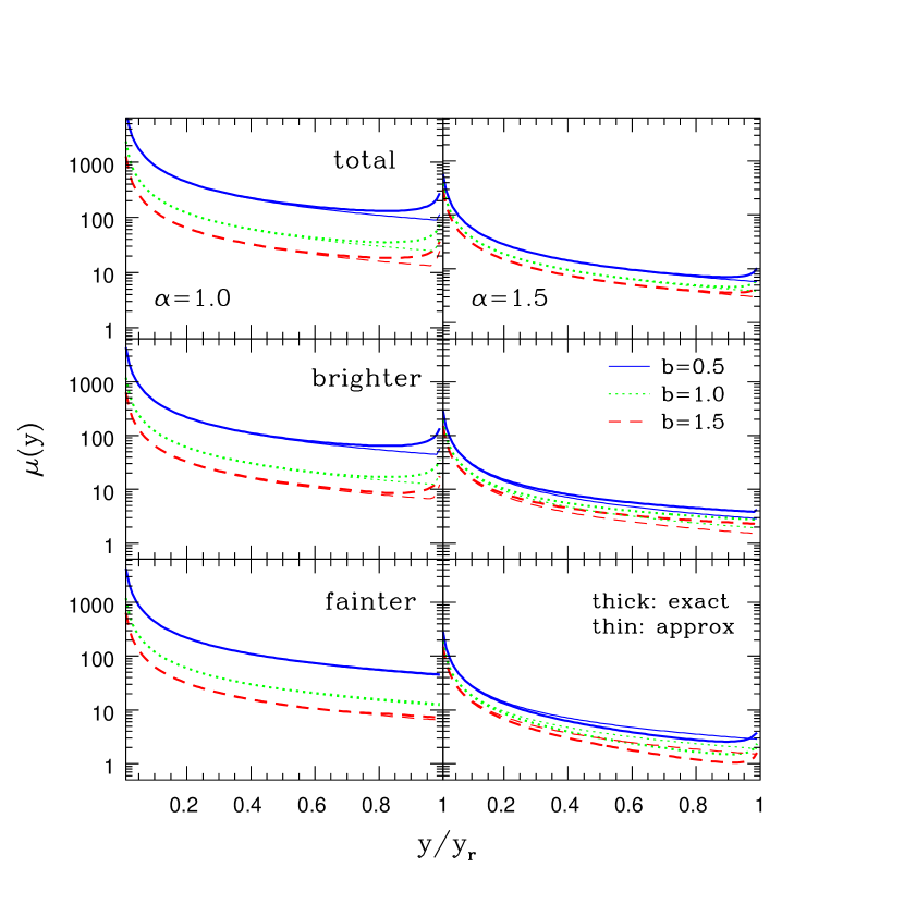
Figure 2: The magnification and its approximation defined in §2.3.2 for generalized NFW profiles with various parameters $b$ and the inner slope $\alpha$. From top to bottom, the magnification is defined by that of the total images, of the brighter and of the fainter image among the outer two images, respectively.

The top panels of Figure 2 shows that the total magnification for the generalized NFW profile is well approximated as (Blandford & Narayan, 1986; Kovner, 1987; Nakamura, 1996)

$$\mu(y) \simeq \left\{\begin{array}[]{@{\hspace{0.6mm}}ll}\hskip 1.70717pt\lx@intercol\displaystyle{\mu_{{\rm t}0}\frac{y_{\rm r}}{y}}&\mbox{$(y<y_{\rm crit})$},\\ \hskip 1.70717pt\lx@intercol\displaystyle{\mu_{{\rm r}0}\frac{1}{(1-y/y_{\rm r})^{1/2}}}&\mbox{$(y>y_{\rm crit})$},\end{array}\right.$$ (23)

where $\mu_{{\rm t}0}$ and $\mu_{{\rm r}0}$ are

$$\mu_{{\rm t}0} = \frac{2x_{\rm t}}{y_{\rm r}(1-bf^{\prime}(x_{\rm t}))},$$ (24)

$$\mu_{{\rm r}0} = \frac{x_{\rm r}}{y_{\rm r}}\sqrt{\frac{2}{y_{\rm r}bf^{\prime\prime}(x_{\rm r})}},$$ (25)

with $x_{\rm r}$ being the position of the radial critical curve. Finally $y_{\rm crit}$ is given by

$$\frac{y_{\rm crit}}{y_{\rm r}}=\frac{-\mu_{{\rm t}0}^{2}+\sqrt{\mu_{{\rm t}0}^{4}+4\mu_{{\rm t}0}^{2}\mu_{{\rm r}0}^{2}}}{2\mu_{{\rm r}0}^{2}}.$$ (26)

The magnification of the brighter or fainter image can be approximated as follows:

$$\mu_{\rm bright}(y) \simeq \left\{\begin{array}[]{@{\hspace{0.6mm}}ll}\hskip 1.70717pt\lx@intercol\displaystyle{\frac{\mu_{{\rm t}0}}{2}\frac{y_{\rm r}}{y}}&\mbox{$(y<y_{\rm crit})$},\\ \hskip 1.70717pt\lx@intercol\displaystyle{\frac{\mu_{{\rm r}0}}{2}\frac{1}{(1-y/y_{\rm r})^{1/2}}}&\mbox{$(y>y_{\rm crit})$},\end{array}\right.$$ (29)

$$\mu_{\rm faint}(y)\simeq\frac{\mu_{{\rm t}0}}{2}\frac{y_{\rm r}}{y}.$$ (30)

Figure 2 shows the comparison between the magnifications of the three cases and their approximation described above (eqs. [23], [29], and [30]). Figure 2 indicates that the above approximation breaks down around its minimum value. In practice, however, this level of discrepancy does not affect the result of the magnification bias (Nakamura, 1996). More importantly, the difference in magnification using total, brighter, or fainter images is only about a factor of two, as easily seen from the above approximations. That is, the different choices of the magnification only increase (or decrease) the probability by a factor of two for all separations. This numerical factor is canceled out in calculating the conditional probability of time delays because it is defined by the ratio of these probabilities (see §3.1). In the SIS case, however, the difference between the magnification of brighter and fainter image is not negligible (see eq. [12]) and as a result the effect of different choice of magnification on time delay probability distributions becomes larger. Therefore, we conclude that the effect of different definitions of the magnification is small in time delay statistics, especially for a small inner slope ($\alpha\lesssim 1.5$).

3 Analytic Formulation of the Time Delay Probability Distribution

3.1 General Formulation

The lens alters the time taken for light to reach the observers and inevitably produces a differential time delay between multiple images (Refsdal, 1964, 1966). The value of the time delay is calculated as (e.g., Schneider et al., 1992)

$$c\Delta t(y)=\frac{\xi_{0}^{2}D_{\rm OS}}{D_{\rm OL}D_{\rm LS}}(1+z_{\rm L})\left[\phi(x^{(1)},y)-\phi(x^{(2)},y)\right],$$ (31)

where $x^{(i)}$ ($i=1,2$) are two image positions. The Fermat potential is written as

$$\phi(x,y)=\frac{(x-y)^{2}}{2}-\psi(x),$$ (32)

in terms of the lensing potential $\psi(x)$. The explicit expressions for the time delays in the SIS and the generalized NFW profiles are given in §3.2.

The cumulative probability of time delays is calculated from equations (7), (8), and (31):

$$P^{\rm B}(>\!\Delta t,\theta;z_{\rm S},L)=\int_{0}^{z_{\rm S}}dz_{\rm L}\,\frac{c\,dt}{dz_{\rm L}}(1+z_{\rm L})^{3}\left[\frac{dM}{d\theta}\pi\,y_{\rm r}^{2}\,\xi_{0}^{2}\,B^{\rm T}(>\!\Delta t;z_{\rm S},L)n(M,z_{\rm L})\right]_{M=M_{\rm min}},$$ (33)

$$B^{\rm T}(>\!\Delta t;z_{\rm S},L)=\left\{\begin{array}[]{@{\hspace{0.6mm}}ll}\hskip 1.70717pt\lx@intercol\displaystyle{\frac{2}{y_{\rm r}^{2}\Phi(z_{\rm S},L)}\int_{y_{\rm min}}^{y_{\rm r}}dy\,y\,\Phi(z_{\rm S},L/\mu(y))\frac{1}{\mu(y)}}&\mbox{($y_{\rm min}<y_{\rm r}$)},\\ \hskip 1.70717pt\lx@intercol\displaystyle{0}&\mbox{($y_{\rm min}>y_{\rm r}$)},\end{array}\right.$$ (36)

where the superscript $T$ on the magnification factor means that the time delay threshold is taken into account. The lower limit of integral $y_{\rm min}$ is determined by solving the equation; $\Delta t=\Delta t(y_{\rm min})$. This expression is valid when the time delay is a monotonic function of the source position $y$ as in all our examples below.

When the magnification bias is neglected, we can replace $B^{\rm T}(>\!\Delta t;z_{\rm S},L)$ by

$$N^{\rm T}(>\!\Delta t)=\left\{\begin{array}[]{@{\hspace{0.6mm}}ll}\hskip 1.70717pt\lx@intercol\displaystyle{\frac{2}{y_{\rm r}^{2}}\int_{y_{\rm min}}^{y_{\rm r}}dy\,y=1-\left(\frac{y_{\rm min}}{y_{\rm r}}\right)^{2}}&\mbox{($y_{\rm min}<y_{\rm r}$)},\\ \hskip 1.70717pt\lx@intercol\displaystyle{0}&\mbox{($y_{\rm min}>y_{\rm r}$)}.\end{array}\right.$$ (39)

The cumulative conditional probability can be calculated from equations (6) and (33):

$$P^{\rm B}(>\!\Delta t\,|\,\theta;z_{\rm S},L)=\frac{P^{\rm B}(>\!\Delta t,\theta;z_{\rm S},L)}{P^{\rm B}(\theta;z_{\rm S},L)}.$$ (40)

We define the joint probability distribution of time delays as:

$$P^{\rm B}(\Delta t,\theta;z_{\rm S},L) \equiv -\frac{d}{d(\Delta t)}P^{\rm B}(>\!\Delta t,\theta;z_{\rm S},L)$$ (41)

$$= \int_{0}^{z_{\rm S}}dz_{\rm L}\,\frac{c\,dt}{dz_{\rm L}}(1+z_{\rm L})^{3}\left[\frac{dM}{d\theta}\pi\,y_{\rm r}^{2}\,\xi_{0}^{2}\,B^{\rm T}(\Delta t;z_{\rm S},L)n(M,z_{\rm L})\right]_{M=M_{\rm min}},$$

$$B^{\rm T}(\Delta t;z_{\rm S},L) = \left\{\begin{array}[]{@{\hspace{0.6mm}}ll}\hskip 1.70717pt\lx@intercol\displaystyle{\frac{2}{y_{\rm r}^{2}\Phi(z_{\rm S},L)}\left[\frac{dy}{d(\Delta t)}y\,\Phi(z_{\rm S},L/\mu(y))\frac{1}{\mu(y)}\right]_{y=y_{\rm min}}}&\mbox{($y_{\rm min}<y_{\rm r}$)},\\ \hskip 1.70717pt\lx@intercol\displaystyle{0}&\mbox{($y_{\rm min}>y_{\rm r}$)}.\end{array}\right.$$ (44)

Similarly, when the magnification bias is not taken into account, we replace $B^{\rm T}(\Delta t;z_{\rm S},L)$ by

$$N^{\rm T}(\Delta t)=\left\{\begin{array}[]{@{\hspace{0.6mm}}ll}\hskip 1.70717pt\lx@intercol\displaystyle{\frac{2}{y_{\rm r}^{2}}\left[\frac{dy}{d(\Delta t)}y\right]_{y=y_{\rm min}}}&\mbox{($y_{\rm min}<y_{\rm r}$)},\\ \hskip 1.70717pt\lx@intercol\displaystyle{0}&\mbox{($y_{\rm min}>y_{\rm r}$)}.\end{array}\right.$$ (47)

Finally the conditional probability distribution of time delays is calculated as in equation (40):

$$P^{\rm B}(\Delta t\,|\,\theta;z_{\rm S},L)=\frac{P^{\rm B}(\Delta t,\theta;z_{\rm S},L)}{P^{\rm B}(\theta;z_{\rm S},L)}.$$ (48)

3.2 SIS and Generalized NFW Profiles

The time delay in the SIS case is calculated from the lensing potential, $\psi(x)=|x|$, and equation (31):

$$c\Delta t(y)=32\pi^{2}\left(\frac{v}{c}\right)^{4}\frac{D_{\rm OL}D_{\rm LS}}{D_{\rm OS}}(1+z_{\rm L})y,$$ (49)

In the generalized NFW case, it is useful to adopt the following approximation in calculating the time delay:

$$\phi(x_{3},y)-\phi(x_{1},y)\simeq 2x_{\rm t}y.$$ (50)

The accuracy of this approximation is shown in Figure 1 (Lower panels). In the analysis below, we employ the approximations shown in Figures 1 and 2. From equations (31) and (50), the time delay for the generalized NFW case is given by

$$c\Delta t(y)=\frac{2r_{\rm s}^{2}x_{\rm t}D_{\rm OS}}{D_{\rm OL}D_{\rm LS}}(1+z_{\rm L})y.$$ (51)

4 Results

4.1 Setting the Conditions

In what follows, we consider three representative cosmological models dominated by CDM; Lambda CDM (LCDM) with $(\Omega_{0},\lambda_{0},h,\sigma_{8})=(0.3,0.7,0.7,1.04)$, Standard CDM (SCDM) with $(1.0,0.0,0.7,0.54)$, and Open CDM (OCDM) with $(0.45,0.0,0.7,0.83)$. The amplitude of the mass fluctuation, $\sigma_{8}$, is normalized so as to reproduce the X-ray luminosity and temperature functions of clusters (Kitayama & Suto, 1997).

We calculate the probability distribution of image separations and time delays adopting the detection condition in the JVAS/CLASS survey. The sample of radio sources have a flux distribution with $\Phi(S)\propto S^{-2.1}$ (Rusin & Tegmark, 2001). In this case, magnification bias factors (8) and (36) are simplified and can be written as

$$B(z_{\rm S},L)=\frac{2}{y_{\rm r}^{2}}\int_{0}^{y_{\rm r}}dy\,y\,\left\{\mu(y)\right\}^{\gamma-1},$$ (52)

and

$$B^{\rm T}(>\!\Delta t;z_{\rm S},L)=\left\{\begin{array}[]{@{\hspace{0.6mm}}ll}\hskip 1.70717pt\lx@intercol\displaystyle{\frac{2}{y_{\rm r}^{2}}\int_{y_{\rm min}}^{y_{\rm r}}dy\,y\,\left\{\mu(y)\right\}^{\gamma-1}}&\mbox{($y_{\rm min}<y_{\rm r}$)},\\ \hskip 1.70717pt\lx@intercol\displaystyle{0}&\mbox{($y_{\rm min}>y_{\rm r}$)}.\end{array}\right.$$ (55)

with $\gamma$ being the slope of the radio luminosity function, $\gamma=2.1$. Using the fact that the luminosity function is described by a power-law and the time delay is proportional to the source position (i.e., $\Delta t\propto y$), equations (44) and (47) are also simplified as

$$B^{\rm T}(\Delta t;z_{\rm S},L)=\left\{\begin{array}[]{@{\hspace{0.6mm}}ll}\hskip 1.70717pt\lx@intercol\displaystyle{\frac{2y_{\rm min}^{2}}{\Delta t\,y_{\rm r}^{2}}\left\{\mu(y_{\rm min})\right\}^{\gamma-1}}&\mbox{($y_{\rm min}<y_{\rm r}$)},\\ \hskip 1.70717pt\lx@intercol\displaystyle{0}&\mbox{($y_{\rm min}>y_{\rm r}$)},\end{array}\right.$$ (58)

and

$$N^{\rm T}(\Delta t)=\left\{\begin{array}[]{@{\hspace{0.6mm}}ll}\hskip 1.70717pt\lx@intercol\displaystyle{\frac{2y_{\rm min}^{2}}{\Delta t\,y_{\rm r}^{2}}}&\mbox{($y_{\rm min}<y_{\rm r}$)},\\ \hskip 1.70717pt\lx@intercol\displaystyle{0}&\mbox{($y_{\rm min}>y_{\rm r}$)}.\end{array}\right.$$ (61)

The redshift distribution of the parent population of radio sources is not known in the JVAS/CLASS survey. Thus we fix the source redshift to the mean redshift of a 27 object subsample, $\langle z_{\rm S}\rangle=1.27$ (Marlow et al., 2000). The results are not substantially different if one takes into account the observed redshift distribution of the subsample (Keeton & Madau, 2001).

4.2 Time Delay Probability Distribution

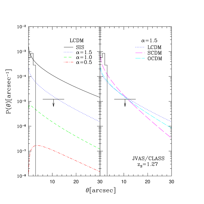
Figure 3: Differential Probability of lensing in the JVAS/CLASS survey. The magnification bias is included. Left panel shows the probability for various density profiles; SIS (solid), generalized NFW with $\alpha=1.5$ (dotted), $\alpha=1.0$ (short dashed), and $\alpha=0.5$ (short dash-dotted). Right panel is the plot for various cosmological models; LCDM (dotted), SCDM (long dashed), and OCDM (long dash-dotted). The observational value is shown by the histogram. The $1\sigma$ constraint from the JVAS/CLASS null result is also shown by a horizontal line with a downward arrow.

Figure 3 plots the predicted probability distribution of image separations for various density profiles (Left panel); SIS, generalized NFW with $\alpha=1.5$, $\alpha=1.0$, and $\alpha=0.5$, and also for various cosmological models (Right panel) fixing $\alpha=1.5$, for reference. As shown in these plots, the probability strongly depends on the inner profile of dark halos. The steeper inner profile produces multiple lenses much more efficiently. The JVAS/CLASS data are also shown in Figure 3. This plot indicates that small separation lensing is consistent with the SIS model, while the SIS model predicts too much large separation lensing, as previously shown by Li & Ostriker (2001).

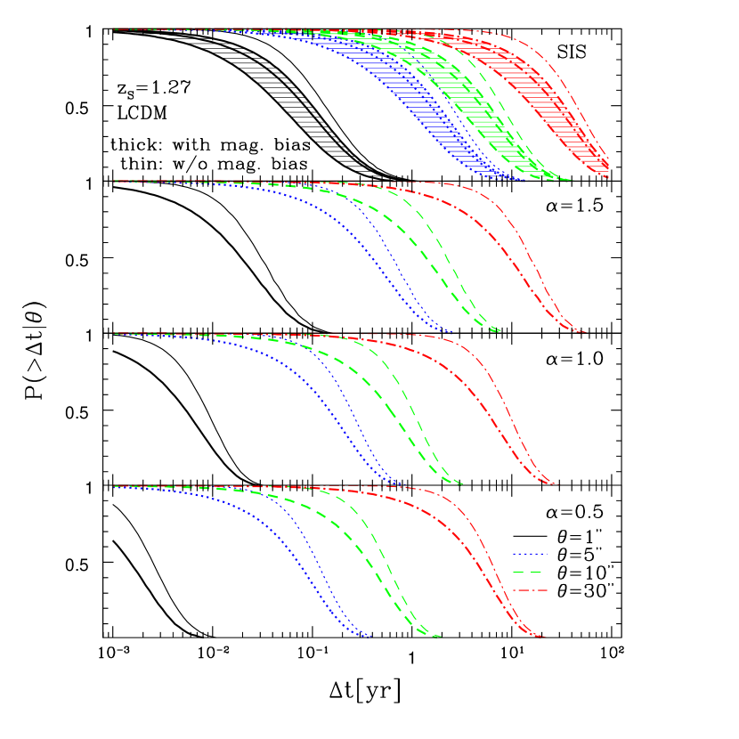
Figure 4: The cumulative conditional probability of time delays (eq. [40]) for various density profiles with image separations $\theta=1^{{}^{\prime\prime}}$ (solid), $5^{{}^{\prime\prime}}$ (dotted), $10^{{}^{\prime\prime}}$ (dashed), and $30^{{}^{\prime\prime}}$ (dash-dotted). The cosmological model is LCDM in each case. Results, with (thick) and without (thin) the magnification bias, are presented. At the top panel, the effect of different choice of magnification is shown by the same three lines and shadings; magnification is defined by that of total images (center lines), of the brighter (right lines) and of the fainter image among the outer two images (left lines).

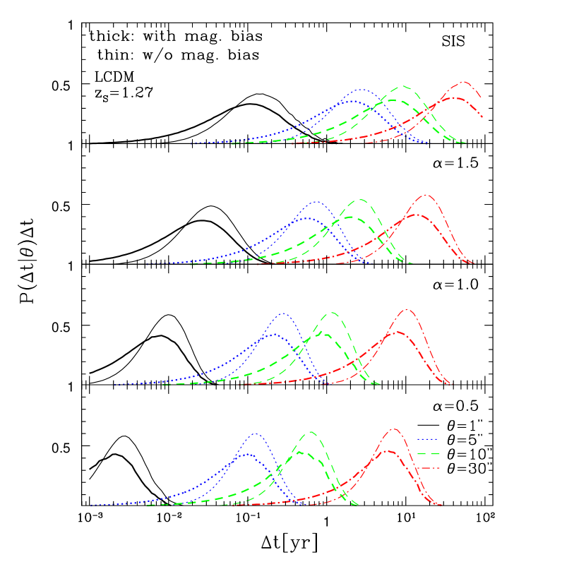
Figure 5: Same as Figure 4, but the differential conditional probability distribution of time delays times $\Delta t$ (eq. [62]) is plotted.

Consider next the time delay probability distributions. Figure 4 plots the cumulative conditional probability (eq. [40]) for different density profiles, and Figure 5 plots its logarithmic time derivative:

$$\frac{d}{d(\ln\Delta t)}P(>\!\Delta t\,|\,\theta;z_{\rm S},L)=P(\Delta t\,|\,\theta;z_{\rm S},L)\Delta t.$$ (62)

The cosmological model is LCDM in each case. We present results both with and without the magnification bias effects. In the Top panel of Figure 4, we plot the three cases of magnification bias defined by that of the total, brighter, and fainter images. The effect of different choice of magnification in the generalized NFW case is smaller than in the SIS case, as discussed in §2.3.2. These plots indicate that time delay statistics depend strongly on the inner slope of the density profile, $\alpha$. Steeper inner profiles tend to produce longer time delays. This is probably because of the deeper gravitational potential for steeper inner profiles. The non-geometric part of the time delay is simply proportional to the difference in the potential value at the image positions. Therefore, we can constrain the density profile of dark halos from this statistics if a reliable and unbiased sample of time delays becomes available.

We note the difference in the asymptotic behavior in the limit of small $\Delta t$ for different magnification biases. For the SIS profile, we obtain the asymptotic behavior of the conditional probability distribution in the limit of the small $\Delta t$ from equations (13), (49) and (58):

$$P(\Delta t\,|\,\theta;z_{\rm S},L)\propto(\Delta t)^{2-\gamma}.$$ (63)

For the generalized NFW profile, we also obtain the same relation from equations (23), (51) and (58). The asymptotic behavior (63) indicates that the uncertainty in the slope of the QSO luminosity function severely affects the probability of shorter time delays. We are not concerned with details of $P(\Delta t\,|\,\theta)$ at small $\Delta t$, where various uncertainties such as the finite size of the sources may affect the shape of $P(\Delta t\,|\,\theta)$ anyway. Except for the small $\Delta t$ regime, however, the uncertainty of the magnification bias is negligible and the time delay probability distribution depends primarily on the inner slope of lens density profile. In fact, the cumulative conditional probability $P(>\!\Delta t\,|\,\theta)$ with or without magnification bias is quite similar and probably observationally indistinguishable for the foreseeable future. In particular, the insensitivity of magnification bias shown in Figures 4 and 5 is in marked contrast with the usual lensing probability as a function of image separation which is affected by more than one order of magnitude (Wyithe et al., 2001; Li & Ostriker, 2001; Takahashi & Chiba, 2001).

To see the dependence of separations and density profiles on the conditional probability distributions more clearly, we calculate the median time delays $\Delta t_{\rm med}$ as follows:

$$P(>\!\Delta t_{\rm med}\,|\,\theta;z_{\rm S},L)=\frac{1}{2}.$$ (64)

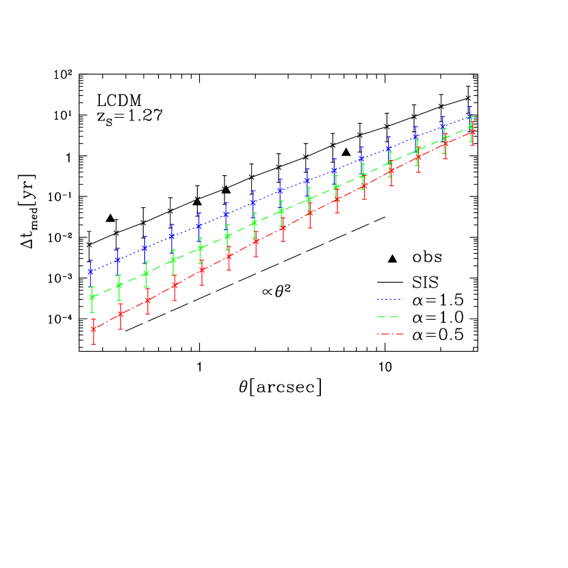
Figure 6: Median time delays, $\Delta t_{\rm med}$, as a function of separations $\theta$, for various density profiles. The median is calculated by equation (64). The error-bars in this plot are defined by the $\pm 25\%$ level. A line with $\Delta t\propto\theta^{2}$ is also shown for reference. Some observational data (see Table 2) are indicated by triangles.

We plot the $\Delta t_{\rm med}$ as a function of separations $\theta$ in Figure 6. The comparison with the observation in this figure will be discussed in §4.3. The error-bars in this plot are defined by the $\pm 25\%$ level. This figure shows that the median time delays are well fitted by the power-law:

$$\Delta t_{\rm med}=A(\theta/1^{{}^{\prime\prime}})^{B}.$$ (65)

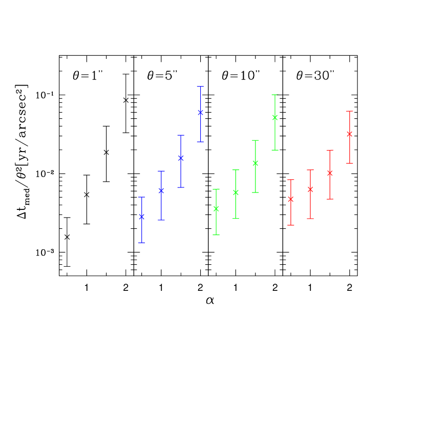
Figure 7: Dependence of time delays on inner slope $\alpha$. Median time delays divided by the square of the separations, $\Delta t_{\rm med}/\theta^{2}$, are plotted. In this plot, the SIS is regarded as $\alpha=2.0$. The error-bars are the same as in Figure 6.

The best-fit values for $A$ and $B$ are summarized in Table 1. Since $B\sim 2$ for all density profiles, Figure 7 plots $\Delta t_{\rm med}/\theta^{2}$ to illustrate their strong dependence on $\alpha$. It is clear in this figure that the difference of $\Delta t_{\rm med}$ between profiles with various $\alpha$ values is larger for smaller separations. To probe the density profile of dark halos, however, small separation lenses may suffer from the complex physics on baryonic components. Therefore lenses with $5^{{}^{\prime\prime}}\lesssim\theta\lesssim 10^{{}^{\prime\prime}}$, which are typically associated with galaxy groups or clusters, may be more useful in constraining the density profile of dark halos. Figure 7 also indicates that it is difficult to determine the inner slope from a single observed lensing system, and several lensing systems are required to reduce the statistical uncertainty.

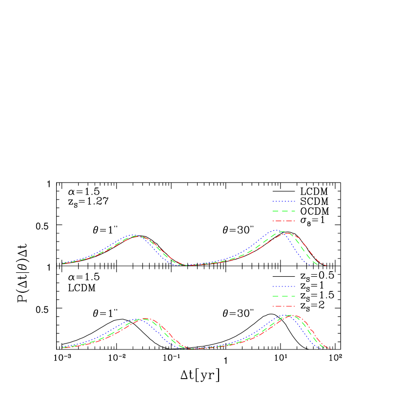
Figure 8: Dependence of the conditional probability distribution of time delays on cosmological model and source redshift. A generalized NFW density profile with $\alpha=1.5$ is adopted. In the upper panel, the cosmological models are LCDM (solid) , SCDM (dotted), and OCDM (dashed). Dash-dotted lines are also for SCDM case, but in this case $\sigma_{8}=1$ instead of $\sigma_{8}=0.54$. In the lower panel, source redshifts $z_{\rm S}=0.5$ (solid), $z_{\rm S}=1.0$ (dotted), $z_{\rm S}=1.5$ (dashed), and $z_{\rm S}=2.0$ (dash-dotted) are plotted.

Next consider the dependence of the statistics on cosmological models or source redshift. Figure 8 displays the predictions for different models and source redshifts, indicating that their effects are rather small. In particular, we emphasize that the time delay probability distribution is insensitive to $\sigma_{8}$, while the SCDM model with $\sigma_{8}=1$ yields nearly two orders more multiple lenses compared with $\sigma_{8}=0.54$. The time delay probability distribution is also insensitive to the redshift uncertainty, especially at high redshift $z_{\rm S}\gtrsim 1$. Therefore, uncertainties of both cosmological models and redshift are not a significant source of uncertainty in time delay statistics. This robustness is also an advantage of time delay statistics compared with the usual overall lensing rate statistic.

4.3 Comparison with Existing Observational Data

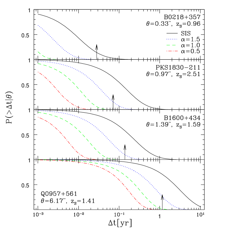
Figure 9: Comparison of predictions with existing time delay data using a cumulative conditional probability. The sample of the lens systems used here is summarized in Table Strong Gravitational Lensing Time Delay Statistics and the Density Profile of Dark Halos. Arrows show the observed values of the time delay in each system. Theoretical predictions with various density profiles are displayed by lines; SIS (solid), generalized NFW with $\alpha=1.5$ (dotted), $\alpha=1.0$ (dashed), and $\alpha=0.5$ (dash-dotted). In calculating the theoretical distributions, the LCDM model was assumed.

Here we tentatively compare our theoretical results with the existing observational data, although the detailed modeling is already available for each system in our small sample. The adopted data are summarized in Table Strong Gravitational Lensing Time Delay Statistics and the Density Profile of Dark Halos. We use time delay data for two images systems and exclude the four image lens systems for simplicity. The data points in Figure 6 and Figure 9 show the comparison with observations for four lens systems. Although Figure 9 displays a more direct comparison, Figure 6 may be useful also in examining whether there is any dependence of the inner slope $\alpha$ on the mass of the lensing objects. For Figure 6, we fix the source redshift at $z_{\rm S}=1.27$, although the source redshift for each system is already known. This does not make any substantial differences as indicated in Figure 8. We plot the theoretical predictions of SIS and generalized NFW density profiles. Observational time delays are indicated by triangles (in Fig. 6) and arrows (in Fig. 9). From these plots, we find that the existing data prefer the steeper inner profiles, SIS profile or generalized NFW profile with $\alpha=1.5$. Although a different choice of magnification affects the median time delays by at most a factor of two (see Fig. 4) in the SIS case and less in the generalized NFW case, this is smaller than the error-bars of median time delays and does not change our basic conclusion. The steep density profiles we infer are also consistent with the detailed models (e.g., Keeton et al., 2000) of these particular lens systems. Of course, the image separations in the lens sample considered here correspond to the inner regions of the lensing galaxies where a plethora of evidence (especially rotation curves) already lead us to expect a roughly isothermal distribution of the total mass, luminous and dark combined, so the results are hardly surprising.

5 Summary and Discussions

In this paper, we formulated the differential time delay probability distribution and examined its dependence on lens density profiles as well as on magnification bias, cosmological model, and source redshift. We found that the probability distribution of time delays depends most sensitively on the inner slope of the lens density profiles. The difference between the various density profiles we examined is very large, more than one order. For example, if $H_{0}=70\,{\rm km/s/Mpc}$, $\Lambda$-dominated cosmology and a source redshift $z_{\rm S}=1.27$ are assumed, lenses with $\theta=5^{{}^{\prime\prime}}$ induce the time delay; $\Delta t[{\rm yr}]=1.5^{+1.7}_{-0.9}$, $0.39^{+0.37}_{-0.22}$, $0.15^{+0.11}_{-0.09}$, and $0.071^{+0.054}_{-0.038}$ (50% level), for SIS, generalized NFW with $\alpha=1.5$, $\alpha=1.0$, and $\alpha=0.5$, respectively.

On the other hand, the effects of cosmological models, source redshifts or magnification bias are rather small, aside from the well known and important linear dependence on the inverse Hubble constant. Moreover, the delay distributions are quite insensitive to the normalization of the overall lensing rate, because the conditional probability is defined by the joint probability divided by the usual lensing probability and the differing of normalizations are almost canceled out. Therefore, one could strongly constrain the core structure of dark halos if a large sample of time delays becomes available in future systematic survey.

Although existing lens systems are individually modeled in detail including the central density profiles, such careful treatment of each lens system in upcoming very large samples may not always be practical. Thus a statistical treatment of time delays is informative. For example, we can predict the range of probable time delays of large separation lenses from this formulation if the density profile of dark halos is fully settled. This would allow estimation of a plausible range of time delays for future lens systems even when the lensing object has not been identified.

Comparison with the meager existing observational data suggests that the density profile has a rather steep cusp, $\alpha\sim 2$, although it is already known that the current observed systems are dominated by baryonic component. Moreover, it seems that the smaller separation lenses prefer steeper inner profiles. This result may support a two-population model, i.e., galactic mass halos with a steep inner slope ($\alpha\sim 2$) and cluster mass halos with a shallower inner slope ($\alpha\lesssim 1.5$), as proposed by Keeton (1998) (see also Porciani & Madau, 2000; Li & Ostriker, 2001). To see whether there are two (or more) populations of halos, time delay data for various separations, especially separations with $5^{{}^{\prime\prime}}\lesssim\theta\lesssim 10^{{}^{\prime\prime}}$, will be essential.

Another application of time delay statistics is that future large samples of lenses will probably be systematically monitored by one or more of the ambitious synoptic surveys now being planned. Designing an efficient sampling rate and observing strategy requires an idea of the range of time delays that might reasonably be expected.

Table 1: Fitting Parameters of Median Time Delays

Model	$A$[yr]	$B$
SIS	$8.05\times 10^{-2}$	1.77
$\alpha$=1.5	$1.91\times 10^{-2}$	1.86
$\alpha$=1.0	$5.37\times 10^{-3}$	2.05
$\alpha$=0.5	$1.48\times 10^{-3}$	2.38

Note. — Fitting Parameters $A$ and $B$ are defined in equation (65)

Table 2: Observed Time Delays for Lenses with Two Images

Lens	$z_{\rm S}$	$\Delta t$ [yr]	$\theta$	Ref.
B0218$+$357	0.96	0.028 $\pm$ 0.004	$0.33^{{}^{\prime\prime}}$	1, 2
PKS1830$-$211	2.51	0.071 $\pm$ 0.014	$0.97^{{}^{\prime\prime}}$	3, 4
B1600$+$434	1.59	0.139 $\pm$ 0.011	$1.39^{{}^{\prime\prime}}$	5, 6
Q0957$+$561	1.41	1.157 $\pm$ 0.002	$6.17^{{}^{\prime\prime}}$	7, 8

References. — (1) Cohen et al. 2000; (2) Biggs et al. 1999; (3) Lovell et al. 1998; (4) Lehár et al. 2000; (5) Burud et al. 2000; (6) Koopmans et al. 2000; (7) Oscoz et al. 2001; (8) Kundić et al. 1997

References

- Barkana et al. (1999) Barkana, R., Lehár, J., Falco, E. E., Grogin, N. A., Keeton, C. R., & Shapiro, I. I. 1999, ApJ, 520, 479
- Biggs et al. (1999) Biggs, A. D., Browne, I. W. A., Helbig, P., Koopmans, L. V. E., Wilkinson, P. N., & Perley, R. A. 1999, MNRAS, 304, 349
- Blandford & Narayan (1986) Blandford, R. D., & Narayan, R. 1986, ApJ, 310, 568
- Browne & Myers (2001) Browne, I. W. A., & Myers, S. T. 2001, in IAU Symp. 201, New Cosmological Data and the Values of the Fundamental Parameters, ed. A. Lasenby, A. Wilkinson, & A. W. Jones, (San Francisco: ASP), 47
- Bullock et al. (2001) Bullock, J. S., Kolatt, T. S., Sigad, Y., Somerville, R. S., Kravtsov, A. V., Klypin, A. A., Primack, J. R., & Dekel, A. 2001, MNRAS, 321, 559
- Burud et al. (2000) Burud, I., et al. 2000, ApJ, 544, 117
- Cen et al. (1994) Cen, R., Gott, J. R., Ostriker, J. P., & Turner, E. L. 1994, ApJ, 423, 1
- Cohen et al. (2000) Cohen, A. S., Hewitt, J. N., Moore, C. B., & Haarsma, D. B. 2000, ApJ, 545, 578
- Fox & Pen (2001) Fox, D. C., & Pen U. L. 2001, ApJ, 546, 35
- Freedman et al. (2001) Freedman, W. L., et al. 2001, ApJ, 553, 47
- Fukushige & Makino (2001a) Fukushige, T., & Makino, J. 2001a, ApJ, 557, 533
- Fukushige & Makino (2001b) Fukushige, T., & Makino, J. 2001b, ApJ, submitted (astro-ph/0108014)
- Grogin & Narayan (1996) Grogin, N. A., & Narayan, R. 1996, ApJ, 464, 92
- Helbig (2000) Helbig, P. 2000, preprint (astro-ph/0008197)
- Hinshaw & Krauss (1987) Hinshaw, G., & Krauss, L. M. 1987, ApJ, 320, 468
- Impey et al. (1998) Impey, C. D., Falco, E. E., Kochanek, C. S., Lehár, J., McLeod, B. A., Rix, H.-W., Peng, C. Y., & Keeton, C. R. 1998, ApJ, 509, 551
- Jing (2000) Jing, Y. P. 2000, ApJ, 535, 30
- Jing & Suto (2000) Jing, Y. P., & Suto, Y. 2000, ApJ, 529, L69
- Keeton (1998) Keeton, C. R. 1998, Ph. D. thesis, Harvard Univ.
- Keeton et al. (2000) Keeton, C. R., et al. 2000, ApJ, 542, 74
- Keeton & Madau (2001) Keeton, C. R., & Madau, P. 2001, ApJ, 549, L25
- Kitayama & Suto (1996) Kitayama, T., & Suto, Y. 1996, ApJ, 469, 480
- Kitayama & Suto (1997) Kitayama, T., & Suto, Y. 1997, ApJ, 490, 557
- Kochanek & White (2001) Kochanek, C. S., & White, M. 2001, ApJ, 559, 531
- Koopmans et al. (2000) Koopmans, L. V. E., de Bruyn, A. G., Xanthopoulos, E., & Fassnacht, C. D. 2000, A&A, 356, 391
- Kovner (1987) Kovner, I. 1987, ApJ, 321, 686
- Kundić et al. (1997) Kundić, T., et al. 1997, ApJ, 482, 75
- Lehár et al. (2000) Lehár, J., et al. 2000, ApJ, 536, 584
- Li & Ostriker (2001) Li, L. X., & Ostriker, J. P. 2001, ApJ, in press (astro-ph/0010432)
- Lovell et al. (1998) Lovell, J. E. J., Jauncey, D. L., Reynolds, J. E., Wieringa, M. H., King, E. A., Tzioumis, A. K., McCulloch, P. M., & Edwards, P. G. 1998, ApJ, 508, L51
- Marlow et al. (2000) Marlow, D. R., Rusin, D., Jackson, N., Wilkinson, P. N., Browne, I. W. A., & Koopmans, L. 2000, AJ, 119, 2629
- Meneghetti et al. (2001) Meneghetti, M., Yoshida, N., Bartelmann, M., Moscardini, L., Springel, V., Tormen, G., & White S. D. M. 2001, MNRAS, 325, 435
- Molikawa & Hattori (2001) Molikawa, K., & Hattori, M. 2001, ApJ, 559, 544
- Moore et al. (1999) Moore, B., Quinn, T., Governato, F., Stadel, J., & Lake, G. 1999, MNRAS, 310, 1147
- Nakamura (1996) Nakamura, T. T. 1996, Master’s thesis, Univ. of Tokyo
- Nakamura & Suto (1997) Nakamura, T. T., & Suto, Y. 1997, Prog. Theor. Phys., 97, 49
- Navarro, Frenk, & White (1996) Navarro, J. F., Frenk, C. S., & White, S. D. M. 1996, ApJ, 462, 563
- Navarro, Frenk, & White (1997) Navarro, J. F., Frenk, C. S., & White, S. D. M. 1997, ApJ, 490, 493
- Oguri et al. (2001) Oguri, M., Taruya, A., & Suto, Y. 2001, ApJ, 559, 572
- Oscoz et al. (2001) Oscoz, A., et al. 2001, ApJ, 552, 81
- Phillips et al. (2001) Phillips, P. M., Browne, I. W. A., & Wilkinson, P. N. 2001, MNRAS, 321, 187
- Phillips et al. (2000) Phillips, P. M., Browne, I. W. A., Wilkinson, P. N., & Jackson, N. J. 2000, preprint (astro-ph/0011032)
- Porciani & Madau (2000) Porciani, C., & Madau, P. 2000, ApJ, 532, 679
- Press & Schechter (1974) Press, W. H., & Schechter, P. 1974, ApJ, 187, 425
- Refsdal (1964) Refsdal, S. 1964, MNRAS, 128, 307
- Refsdal (1966) Refsdal, S. 1966, MNRAS, 132, 101
- Rusin (2000) Rusin, D. 2000, preprint (astro-ph/0004241)
- Rusin & Tegmark (2001) Rusin, D., & Tegmark, M. 2001, ApJ, 553, 709
- Sasaki & Takahara (1993) Sasaki, S., & Takahara, F. 1993, MNRAS, 262, 681
- Schneider et al. (1992) Schneider, P., Ehlers, J., & Falco, E. E. 1992, Gravitational Lenses (New York: Springer)
- Takahashi & Chiba (2001) Takahashi, R., & Chiba, T. 2001, ApJ, in press (astro-ph/0106176)
- Turner (1980) Turner, E. L. 1980, ApJ, 242, L135
- Turner, Ostriker, & Gott (1984) Turner, E. L., Ostriker, J. P., & Gott, J. R. 1984, ApJ, 284, 1
- Williams, Navarro, & Bartelmann (1999) Williams, L. L. R., Navarro, J. F., & Bartelmann, M. 1999, ApJ, 527, 535
- Witt, Mao, & Keeton (2000) Witt, H. J., Mao, S., & Keeton, C. R. 2000, ApJ, 544, 98
- Wyithe et al. (2001) Wyithe, J. S. B., Turner, E. L., & Spergel, D. N. 2001, ApJ, 555, 504