A Non-parametric Analysis of the CMB Power Spectrum

Abstract

We examine Cosmic Microwave Background (CMB) temperature power spectra from the BOOMERANG, MAXIMA, and DASI experiments. We non-parametrically estimate the true power spectrum with no model assumptions. This is a significant departure from previous research which used either cosmological models or some other parameterized form (e.g. parabolic fits). Our non-parametric estimate is practically indistinguishable from the best fit cosmological model, thus lending independent support to the underlying physics that governs these models. We also generate a confidence set for the non-parametric fit and extract confidence intervals for the numbers, locations, and heights of peaks and the successive peak-to-peak height ratios. At the 95%, 68%, and 40% confidence levels, we find functions that fit the data with one, two, and three peaks respectively ($0\leq\ell\leq 1100$). Therefore, the current data prefer two peaks at the $1\sigma$ level. However, we also rule out a constant temperature function at the $>8\sigma$ level. If we assume that there are three peaks in the data, we find their locations to be within $\ell_{1}$ = (118,300), $\ell_{2}$ = (377,650), and $\ell_{3}$ = (597,900). We find the ratio of the first peak-height to the second $(\frac{\Delta T_{1}}{\Delta T_{2}})^{2}=(1.06,4.27)$ and the second to the third $(\frac{\Delta T_{2}}{\Delta T_{3}})^{2}=(0.41,2.5)$. All measurements are for 95% confidence. If the standard errors on the temperature measurements were reduced to a third of what they are currently, as we expect to be achieved by the MAP and Planck CMB experiments, we could eliminate two-peak models at the 95% confidence limit. The non-parametric methodology discussed in this paper has many astrophysical applications.

1. Introduction

There has been growing evidence for the existence of peaks and valleys in the temperature power spectrum of the CMB. From a theoretical standpoint, such features are a direct result of the physics in the primordial photon-electron plasma, predicted by gravitational instability models of structure formation (Peebles & Yu 1970; Hu and Sugiyama 1995). These features are important for constraining the cosmology of our Universe. For instance, in many models, the ratio of the height of the first peak to the second peak is dependent on the spectral tilt, $n_{s}$ and the baryon fraction, $\Omega_{baryons}/\Omega_{matter}$. The ratio of the third peak to the second peak is dependent on $\Omega_{matter}h^{2}$ and $n_{s}$ (see Hu et al. 2001 for further discussion).

Most often in the literature, the CMB power spectra are fit to a suite of cosmological models (Tegmark et al., 1999,2000; Jaffe et al. 2001). These physical models are well-motivated and sophisticated, but they contain many free parameters (e.g., eleven in the work of Wang, Tegmark, and Zaldarriaga 2001– WTZ), some of which are unknown (ionization depth, contribution from gravity waves) or degenerate (e.g. see Efstathiou 2001). Typically, some sort of likelihood analysis is performed to determine which cosmological model best fits the data.

There is however, another approach: place constraints on the features of the power spectrum and use these features to determine the cosmological parameters. The assumptions here are that the peaks and valleys are best described by the broad range of cosmological models (as in Hu et al.) or by parabolas or some other chosen function (as in Knox & Page 2000 and de Bernardis et al. 2001). A potential problem in all of these approaches is that it is difficult to get valid statistical confidence intervals (see Section 2). There is also the concern that the fitted features may be artifacts from the multitude of assumptions.

In this paper, we take what may be considered a more conservative approach: we make no assumptions whatsoever about the true underlying function. Our new statistical technique is non-parametric and allows for valid confidence intervals to be measured for peak characteristics. One theme of our work is that confidence intervals for any quantity of interest can be extracted from a confidence set for the unknown spectrum. These techniques for fitting and inference are applicable to a wide variety of astrophysical data-analysis problems.

2. Overview of Nonparametric Analysis

In general, non-parametric statistical methods estimate functions without imposing a finite-dimensional parametric form. The resulting estimates are obtained by carefully smoothing the data to balance bias and variance. See Hastie and Tibshirani (1990) for details and examples.

The CMB data, after suitable preprocessing, take the form $(X_{1},Y_{1}),\ldots,(X_{n},Y_{n})$ where $X_{i}$ is the multipole moment (usually denoted $\ell$) ordered according to increasing $X$, and $Y_{i}$ is the estimated power spectrum at $X_{i}$ (usually denoted $C_{\ell}$ with some constants). Let $f(X_{i})$ be the true power spectrum at $X_{i}$. Then,

$$Y_{i}=f(X_{i})+\epsilon_{i}$$ (1)

where $\epsilon_{i}$ is the error in estimating $f(X_{i})$. We require that the $\epsilon_{i}$ are uncorrelated, zero-mean Gaussians. Therefore, we take the uncorrelated statistical errors as given by the experiments. There are additional, correlated noise terms in all of the experiments due to calibration, beam width and pointing uncertainties, which were not used in our analysis. The magnitude of these correlated errors is typically 5% - 20%, although the Boomerang effective beam uncertainties can be higher for $\ell>600$. The method we use in this work can be generalized to include correlated errors (Genovese et al., in preparation). We assume that $f^{2}$ is integrable; otherwise, we make no further assumptions. Our non-parametric technique yields a vector $\widehat{\bf f}$ that estimates the vector ${\bf f}=(f(X_{1}),\ldots,f(X_{n}))$ of the true spectrum’s values at the $X_{i}$s (see Figure 1 top).

After we perform the fit, we need to quantify the uncertainty to make any inferences. We begin by constructing a set of vectors $C_{n}$ from the data that traps the true power spectrum, $\bf f$, with probability $1-\alpha$, where $1-\alpha$ is a pre-specified confidence level. With $C_{n}$ we can derive a confidence interval for any quantity of interest. Consider, for example, the number of peaks. For any vector ${\bf f}\in C_{n}$, define $P({\bf f})$ to be the number of peaks in ${\bf f}$. Then, because $C_{n}$ contains the true spectrum with confidence $1-\alpha$, the range on the measured peaks is $\left(\min_{{\bf f}\in C_{n}}P({\bf f}),\max_{{\bf f}\in C_{n}}P({\bf f})\right)$. We can find confidence intervals for the locations and heights of peaks in a similar way. There are important advantages for these confidence measurements over “standard” $\chi^{2}$ or even Bayesian techniques, which we discuss further in the next section.

3. Methodology

Refer to the model in equation (1). Let the functions $\phi_{1},\phi_{2},\ldots$ be an orthonormal basis over the range of the observed $X_{i}$s. The choice of basis is somewhat important. For instance, if we were fitting to a galaxy spectrum, with highly peaked emission lines on top of a smooth, broad continuum, a wavelet basis would allow for the simultaneous fitting of broad and narrow features. On the other hand, a cosine basis would require large amplitude high frequency terms to match the emission lines. This might cause the continuum fit to be wiggly. In our work, we use a discrete cosine basis, $\phi_{1}(x)\equiv 1$, $\phi_{2}(x)=\sqrt{2}cos(\pi x)$, $\phi_{3}(x)=\sqrt{2}cos(2\pi x),\ldots$, since it has well determined properties for confidence limits. For simplicity in the derivation, we assume that the variance (second moment about the mean) of each $\epsilon_{i}$ is the same value $\sigma^{2}$. This is not necessary in practice, nor was it assumed in the full analysis.

Any square integrable function $f$ can be expanded as $f(x)=\sum_{j=1}^{\infty}\beta_{j}\phi_{j}(x)$. Estimating $f$ amounts to estimating the $\beta_{j}$’s. If we have chosen a good basis for representing $f$, the higher-order terms in this series will tend to decay rapidly. Hence, we can approximate the infinite sum with finite sum $f(x)\approx\sum_{j=1}^{N}\beta_{j}\phi_{j}(x)$. So, to estimate the underlying function, we need to find the $\beta$s.

Let $Z_{j}=N^{-1/2}\sum_{i=1}^{N}Y_{i}\phi_{j}(X_{i})$, for $j=1,\ldots,N$. Based on the theory in Beran (2000), we take $N=n$. This choice ensures that the estimate of $f$ is optimal and that the resulting confidence intervals remain valid. It can be shown that each statistic $Z_{j}$ has approximately a Gaussian distribution with mean $\theta_{j}=\sqrt{n}\beta_{j}$ and variance $\sigma^{2}$. This re-parameterization means that we need to estimate $\theta=(\theta_{1},\ldots,\theta_{n})$. Given an estimate $\widehat{\theta}$ of $\theta$, we can estimate $f(X_{i})$ via $\widehat{f}(X_{i})=(1/\sqrt{n})\sum_{j=1}^{n}\widehat{\theta}_{j}\phi_{j}(X_{i})$.

We could use $Z_{j}$ as an estimate of $\theta_{j}$, but this yields a poor estimate of $f$ because it is too variable. A smoother estimate can be obtained by damping the higher frequency terms in the expansion. In statistics, this is called a “shrinkage estimator”. We consider shrinkage estimators of the form $\widehat{\theta}=(\gamma_{1}\,Z_{1},\gamma_{2}\,Z_{2},\cdots,\gamma_{n}\,Z_{n})$, where $1\geq\gamma_{1}\geq\gamma_{2}\geq\cdots\geq\gamma_{n}\geq 0$ are called the shrinkage coefficients. The smaller $\gamma_{j}$, the smaller the contribution of $\phi_{j}$ in the estimating expansion for $f$. With the cosine basis, for example, such shrinkage estimators damp down the contribution from high-frequency terms.

Every choice of $\gamma=(\gamma_{1},\ldots,\gamma_{n})$ gives an estimate $\widehat{\theta}^{\gamma}$ which then yields an estimate $\widehat{f}^{\gamma}$ of the function $f$. We would like to choose $\gamma$ to minimize the mean squared error, ${\rm MSE}(\gamma)=\langle\int(f(x)-\widehat{f}^{\gamma}(x))^{2}dx\rangle$. Unfortunately ${\rm MSE}(\gamma)$ is unknown, because it depends on the true $f$, but it can be estimated by Stein’s Unbiased Risk Estimator (Stein 1981):

$$\widehat{{\rm MSE}}(\gamma)=\sum_{j}\left[\sigma^{2}\gamma^{2}_{j}+\left(Z_{j}^{2}-\sigma^{2}\right)(1-\gamma_{j})^{2}\right].$$ (2)

We use the Pooled Adjacent Values (PAV) algorithm (Robertson, Wright, and Dykstra, 1988) to minimize $\widehat{{\rm MSE}}(\gamma)$ as a function of $\gamma$ while maintaining the ordering constraint on $\gamma$. The minimizer is denoted $\widehat{\gamma}$ and the final estimate is therefore $\widehat{\theta}=(\widehat{\gamma}_{1}\,Z_{1},\widehat{\gamma}_{2}\,Z_{2},\cdots,\widehat{\gamma}_{n}\,Z_{n})$.

Next we construct a confidence set, $C_{n}$ for the vector of function values at the observed data, ${\bf f}_{n}=(f(X_{1}),f(X_{2}),\cdots,f(X_{n}))$. Throughout the paper we have said that the confidence sets are “valid.” Formally, what this means is that for any $c>0$,

$$\lim_{n\rightarrow\infty}~{}\sup_{||{\bf f}_{n}||\leq c}\left|{\rm Pr}({\bf f}_{n}\in C_{n})-(1-\alpha)\right|\rightarrow 0$$ (3)

as $n\rightarrow\infty$, where the operation $||a||$ denotes $\sqrt{n^{-1}\sum_{i}a_{i}^{2}}$. This means that for large $n$, the confidence set traps the values of the true function with probability very close to $1-\alpha$. The confidence set is an ellipse of the form

$$C_{n}=\left\{\theta:\ n^{-1}\sum_{j}(\theta_{j}-\widehat{\theta}_{j})^{2}\leq\widehat{MSE}(\widehat{\gamma})+n^{-1/2}\tau z_{\alpha}\right\}$$ (4)

where $z_{\alpha}$ is the number that has probability $\alpha$ to the right under a standard Gaussian. For instance, if we choose 95% confidence ($\alpha=0.05$), then $z_{\alpha}=1.645$, while for 67% confidence ($\alpha=0.33$), the confidence “radius” is smaller with $z_{\alpha}=0.44$. Here, $\tau$ is defined similar to Beran (2000):

$$\tau^{2}=4\,\sigma^{2}\,\sum_{j}(Z^{2}_{j}-\sigma^{2})(1-\widehat{\gamma}_{j})^{2}+2\,\sigma^{4}\,\sum_{j}(2\widehat{\gamma}_{j}-1)^{2}.$$ (5)

We can in turn write the confidence set for ${\bf f}$ as

$${\cal D}_{n}=\left\{{\bf f}:\ {\bf f}=n^{-1/2}\,\sum_{j=1}^{n}\theta_{j}\phi_{j}\mbox{ and }\theta\in{\cal C}_{n}\right\}.$$ (6)

Here, the true power spectrum ${\bf f}=(f(X_{1}),...,f(X_{n}))$ is estimated at each of the original data points. Prior information about $\bf f$ of the form ${\bf f}\in{\cal P}_{n}$ allows us to replace ${\cal D}_{n}$ with ${\cal D}_{n}\cap{\cal P}_{n}$ while maintaining a $1-\alpha$ confidence level. In particular, we take ${\cal P}_{n}$ to be the set of vectors ${\bf f}$ corresponding to spectra with zero to three peaks for $\ell\leq 1100$. From the confidence set ${\cal D}_{n}\cap{\cal P}_{n}$, we can derive confidence sets for any interesting feature of ${\bf f}$.

A key point is that the resulting intervals on any measured quantity are simultaneously valid, meaning that all of the intervals contain the corresponding true quantity with probability $1-\alpha$. In contrast, deriving $1-\alpha$ confidence intervals from a collection of individual chi-squares does not obtain $1-\alpha$ simultaneous coverage, but often substantially lower coverage. For example, a common technique to determine the 95% confidence range for a specific parameter is to “marginalize” over the other parameters (see Tegmark et al. 1999,2000). Such a technique will provide full coverage for that one parameter. However, when parameter ranges are combined, the confidence is lower than 95%. Bayesian intervals derived from a posterior distribution suffer from a similar problem in that the long-run frequency that the interval contains the true quantity may be much less than $1-\alpha$.

4. Results

Figure 1 shows the combined data from BOOMERANG, MAXIMA, and DASI (Halverson et al. 2001; Lee et al. 2001; and Netterfield et al. 2001). The bottom panel compares our non-parametric fit to the the fit of WTZ who use more experiments than the three examined here. Recall, our fit requires no assumptions about the data or the underlying cosmology. The WTZ fit, on the other hand, requires an 11 dimensional parameter space, with numerous prior assumptions placed on those parameters (for example, the Hubble constant is constrained to $72\pm{8}$ km s^-1Mpc^-1). The agreement between the two fits is very good, considering the difference in methodology.

The power of this technique lies in the ability to make quantitative statements about the true function with some specified confidence. First, we checked the 95% confidence set and find that every function within this set has at least one peak. Specifically, we set $\alpha=0.05$ and determined the “radius” of this confidence ellipse (ie. the right side of the inequality in Eq 4). We then searched all possible functions with zero to three peaks over the specified range in $\ell$ to see if the condition in Eq 4 was met. Our definition of one peak requires the sorted data (according to increasing $\ell$) to have a section with increasing temperature followed by a section with decreasing temperature. For $\alpha=0.05$, no zero-peaked functions met this condition. Our set of zero-peaked functions includes those with constant temperature as well as those with either increasing temperature or decreasing temperature, but not both. We rule out functional forms with zero peaks at the level 95% confidence level. We also compared specifically against the best fit constant function for the power spectrum. We rule out a flat temperature spectrum (based on the weighted average of the data) at $>8\sigma$ confidence. We perform the same analysis at the 68% confidence level (e.g. $\alpha=0.32$ in Eq 4). The 68% confidence set rules out all single-peak functions. So at the one sigma level, we have found at least two peaks in the data. Only in the 40% ($\alpha=0.6$) confidence set can we rule out two-peak functions. From our confidence sets, the data supports two peaks out of three peaks in the CMB power spectrum (for $0\leq\ell\leq 1100$).

We calculate ranges for the peak heights and locations in Table 1. Figure 2 shows the non-parametric fit with confidence intervals for peak heights and locations at 95% confidence. Finally, we computed confidence intervals for the ratios of successive peaks under a three-peak model. The 95% confidence interval for the ratio of the height of the first peak to the height of the second peak is $(1.06,4.27)$. The 95% confidence interval for the ratio of the height of the second peak to the height of the third peak is $(0.41,2.5)$. This rules out equal heights for the first two peaks at the 95% level. These results are consistent with Hu et al. (2001) who find much stronger constraints on the height-height ratios by fitting to cosmological models.

5. Discussion and Conclusions

We present an application of a new and powerful non-parametric technique to CMB temperature data. Past approaches were based on complicated cosmological models or parameterized forms. There is superb visual agreement between the non-parametric fit and the best fitting cosmological model. Quantitatively, we provide constraints on the peak locations, heights, and height ratios of the power spectrum. These constraints can be used to place corresponding limits on the cosmological parameters that they describe. For instance, Hu et al. (2001) derive relationships which could in principle, be used for this purpose.

At the $2\sigma$ confidence level, we find at least one peak in the current CMB power spectra data, while at the $1\sigma$ level, we find two or more peaks. Only for a very low confidence, 40%, can we rule out two peak functions. Therefore, the data do not yet show the three expected peaks for $\ell\leq 1100$ (in the three CMB datasets examined here). There are two explanations for this: the model is right, but there is insufficient precision in the current data, or the model is wrong. If in fact the errors on the current measurements are simply too large, then these standard errors would have to be reduced to one-third of their current values to rule out a two-peak spectrum at the 95% confidence level. This suggests a range for the maximum required errors for future CMB experiments (via MAP and Planck) to “discover” three peaks in the CMB spectrum.

We point out that the lack of assumptions used to arrive at our best fit is conservative. On the other hand, results from fitting assumed cosmological models are optimistic, since those models all have a multi-peaked spectra (e.g. Hu et al. 2001). While the physical underpinnings for cosmological models are well founded, the last 50 years (or even five) have seen radical changes in those models which best fit the data. Therefore, a method to describe the CMB that is “cosmology free” has scientific value. Finally, we note that the methods described here can be applied to the many astrophysical problems that are not well suited for standard parametric techniques.

This work was done in collaboration with the Pittsburgh Computational Astrostatistics Group (www.picagroup.org). The authors would like to thank the referee for suggestions which improved the readability and usefulness of this work. RCN, LW, and CG were partially supported by NSF KDI grant DMS-9873442.

During the refereeing process of our paper, two related papers came to our attention (Durrer, Novosyadlyj & Apunevych 2001; Douspis & Ferreira 2001). These papers perform a model–independent measurement of the CMB power spectrum but they are not non-parametric estimates of the CMB acoustic peaks, as discussed herein, since they use phenomenological models to describe the underlying power spectrum. It is interesting to note however, that all three analyses find low statistical significances for the detection of the second and third peaks. We await higher precision measurements of the CMB power spectrum to secure the detection, location, shape and amplitude of these peaks.

Table 1Three Peak Confidence Intervals

Peak	Location	Height
1	(118,300)	(4361,8055)
2	(377,650)	(1829,4798)
3	(597,900)	(1829,4688)

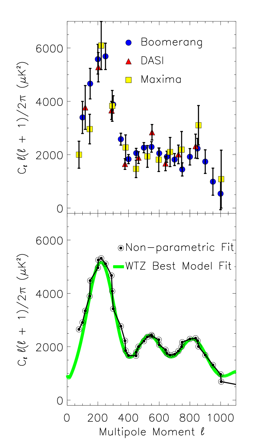
Figure 1.— The top panel shows the raw CMB data from the Boomerang, MAXIMA, and DASI experiments. The middle panel is the raw CMB data over–plotted with the best fit using the non-parametric technique. The bottom panel shows the non-parametric fit against the best cosmological model fit from Wang, Tegmark, and Zaldarriaga (2001).

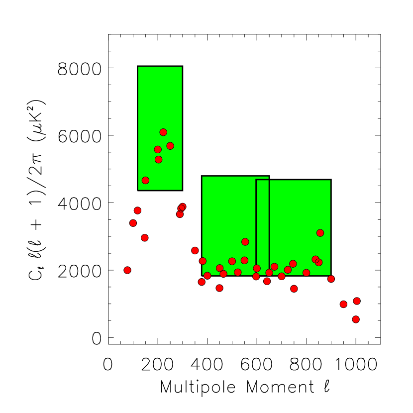
Figure 2.— The ranges on the locations and peak heights of the non-parametric three peak (and two dip) fit function (95% confidence).

References

- de Bernardis (2001) de Bernardis, P., et al. 2001, ApJsubmitted, astro-ph/0105296
- Beran (2000) Beran, R. 2000, J. Amer. Stat. Assoc. 95, 155
- Douspis and Ferreira (2001) Douspis, M. and Ferreira, P. G., 2001, see astro–ph/0111400
- Durrer et al. (2001) Durrer, R., Novosyadlyj, B., Apunevych, S., 2001, ApJ, submitted, see astro-ph/0111594
- Efstathiou (2001) Efstathiou, G. 2001, submitted to MNRAS, astro-ph/0109151
- Halverson et al. (2001) Halverson, N.W., et al. 2001, ApJsubmitted, astro-ph/0104489
- (7) Hastie, T. J. and Tibshirani, R. J. 1990,Generalized Additive Models, Chapman and Hall, London
- Hu & Sugiyama (1996) Hu, W. & Sugiyama, N. 1996, ApJ, 471, 542
- Hu, Fukugita, Zaldarriaga, & Tegmark (2001) Hu, W., Fukugita, M., Zaldarriaga, M., & Tegmark, M. 2001, ApJ, 549, 669
- Jaffe et al. (2001) Jaffe. A., et al. 2001, astro-ph/0007333
- Knox & Page (2001) Knox, L. and Page, L. 2000, Phys. Rev. L., 85, 1366
- Lee et al. (2001) Lee et al. 2001, astro-ph/0104459
- Netterfield et al. (2001) Netterfield et al. 2001, ApJsubmitted, astro-ph/0104460
- Peebles & Yu (1970) Peebles, P. J. E. & Yu, J. T. 1970, ApJ, 162, 815
- Robertson, Wright, & Dykstra (1988) Robertson, T., Wright, F.T., and Dykstra, R.L. 1988, Order Restricted Statistical Inference, Wiley, New York
- Stein (1981) Stein, C. 1981, Ann. of Statist., 9, 1135
- Tegmark (1999) Tegmark, M. 1999, ApJ, 514, L69
- Tegmark & Zaldarriaga (2000) Tegmark, M. & Zaldarriaga, M. 2000, ApJ, 544, 30
- Wang et al. (2001) Wang, X., Tegmark, M. and Zaldarriaga, M. 2001, Phys. Rev. D. submitted, astro-ph/0105091 – WTZ