B1422+231:The influence of mass substructure on strong lensing

In this work we investigate the gravitationally lensed system B1422+231. High-quality VLBI image positions, fluxes and shapes as well as an optical HST lens galaxy position are used. First, two simple and smooth models for the lens galaxy are applied to fit observed image positions and fluxes; no even remotely acceptable model was found. Such models also do not accurately reproduce the image shapes. In order to fit the data successfully, mass substructure has to be added to the lens, and its level is estimated. To explore expectations about the level of substructure in galaxies and its influence on strong lensing, N-body simulation results of a model galaxy are employed. By using the mass distribution of this model galaxy as a lens, synthetic data sets of different four image system configurations are generated and simple lens models are again applied to fit them. The difficulties in fitting these lens systems turn out to be similar to the case of some real gravitationally lensed systems, thus possibly providing evidence for the presence and strong influence of substructure in the primary lens galaxy.

1 Introduction

Gravitational lens systems with multiply imaged quasars are an excellent tool for studying the properties of distant galaxies. In particular, they provide the most accurate mass measures for the lensing galaxy. Besides the mass profiles, one can also gain information about evolution (Kochanek et al. 2000) and extinction laws (Fassnacht et al. 1999). Strong lensing is also a very promising and robust tool to measure the Hubble constant (Refsdal 1964). The success of this method, however, depends strongly on how well the mass model is constrained.

It turns out that image positions can be fit quite accurately with simple, smooth elliptical models (Keeton et al. 1997). Since the number of observational constraints from image positions is small, one wants to include the flux information. The optical fluxes, however, should not be used, as they might be affected by microlensing and/or dust obscuration (Chang & Refsdal 1979). Radio fluxes, on the other hand, can provide further constraints in lens modelling.

Fitting the fluxes very accurately turns out to be difficult in many lens systems. Models for MG0414+0534 (Falco et al. 1997; Keeton et al. 1997), PG1115+080 (Keeton & Kochanek 1997) and B1422+231 (e.g. Kormann et al. 1994) all show the same failure, namely the observed flux ratios are very different from what one would expect for the image configurations from a smooth model. In particular, the gravitational lens system B1422+231 was explored in detail, and as was first mentioned by Mao & Schneider (1998), mass substructure in the lens galaxy might provide an explanation for the failures in flux modelling.

A question arises as to whether there is something special about these quadruple systems, or does the discrepancy simply arise due to the fact that our smooth models are oversimplified? In other words, we are asking how “well” (for the purpose of strong lensing) can the smooth models used to fit the data represent a real galaxy? N-body simulation data can provide a realistic description of a galaxy mass distribution, thus giving a possibility to probe its effect on strong lensing.

In this paper, we will study the influence of the substructure on the lens system B1422+231, using VLBI radio measurements of the system by Patnaik et al. (1999). In Sec. 2 we give a description of the lens system and data used. The method is outlined in Sect. 3 and the results on fitting the system with smooth mass model are presented. In Sect. 5 the model accounting for the substructure is presented and in Sect. 5.2 the deconvolved image shape information is added to the fit. Sect. 6 gives the description of the method used to investigate lensing by an N-body simulated galaxy. We describe how we obtained synthetic data of four image systems, and the results of fitting such systems with lens models are presented. Finally we draw some conclusions in Sect. 7.

This work is an abbreviated version of Bradač (2001). In the course of writing this paper, several related papers on substructure of lens galaxies have been submitted (Metcalf & Madau 2001; Chiba 2001; Dalal & Kochanek 2001; Metcalf & Zhao 2001; Keeton 2001). In Metcalf & Madau (2001) and Chiba (2001), the authors use semi-analytical descriptions to account for mass clumps typical for N-body simulations in a statistical fashion. In addition, Chiba (2001) tests his prediction on two known systems with four images. Dalal & Kochanek (2001), Metcalf & Zhao (2001), and Keeton (2001) predict the properties of substructure needed to constrain lens systems and compare their results with the CDM predictions. In addition, Keeton (2001) accounts for the difference between radio and optical fluxes by investigating radio and optical sources of different sizes. The present work is differs from the afore mentioned in that slightly different models for the lens in B1422+231 system are used and that we also include image shape constraints in the fit. Further, we investigate four image systems generated by using a CDM N-body simulated galaxy, rather than an analytic approximation for the statistics of mass-substructure.

2 The mystery of B1422+231

The gravitational lens system B1422+231 was discovered in the course of the JVAS survey (Jordell Bank – VLA Astrometic Survey) by Patnaik et al. (1992). It consists of four image components. The three brightest images A, B, and C (as designated by Patnaik et al. 1992) are fairly collinear. The radio flux ratio between images A and B is approximately 0.9, while image C is fainter (flux ratio C to B is approximately 0.5). Image D is further away and is much fainter than the other images (with flux ratio D:B of 0.03). The most recent available radio data for the image positions and fluxes were obtained from the polarisation observations made at $8.4\;{\rm GHz}$ using the VLBA and the 100m telescope at Effelsberg from Patnaik et al. (1999) and are listed in Table 1. For each of the components, the authors measured positions (relative to the image B) and fluxes as well as the deconvolved image shapes. Here and through the paper we are using a notation where $(\theta_{1},\theta_{2})$ are the angular coordinates in the lens plane and $(\beta_{1},\beta_{2})$ in the source plane. $\theta_{1}$ and $\beta_{1}$ increase in the negative RA direction.

The radio source of this lens system is associated with a $15.5\;{\rm mag}$ quasar at a redshift of $3.62$ (Patnaik et al. 1992). The lensing galaxy has been observed in the optical; its redshift has been determined to be $0.338$ and its position relative to image B has been measured (Impey et al. 1996). The main lens galaxy is a member of a compact group with a median projected radius of $35\;h^{-1}\;{\rm kpc}$ and velocity dispersion of $\sim 550\;{\rm km\>s^{-1}}$ (Kundic et al. 1997).

Several groups have tried to model B1422+231 (Hogg & Blandford 1994; Kormann et al. 1994; Keeton et al. 1997; Mao & Schneider 1998) and all of them have experienced difficulties in fitting it. As we used data with even more precise image positions one might expect that it would become even harder to model the system. However, as already pointed out by some authors, the difficulties do not lie in fitting the image positions but rather in the flux ratios.

It turns out that simple, smooth models fail to reproduce the radio as well as the optical flux ratios of the system. While the mismatch in optical data might still be due to the microlensing and/or dust obscurations, this can probably not explain why such models are not successful when fitting radio flux ratios. Mao & Schneider (1998) have proposed a lens model that accounts for the substructure in the lensing galaxy. They concluded that one needs a surface mass density perturbation of the order of 1 % of the critical surface mass density in order to change the flux ratios to the observed values.

In order to succeed in fitting the image flux ratios, one needs to consider more sophisticated models. However, such models also require the use of additional parameters. Therefore it is very difficult to ensure a constrained model that accounts for the substructure using as constraints only image positions, flux ratios, and the galaxy position. For this reason we also included the axis ratios and the orientation angles of the deconvolved images as additional constraints. They were obtained from Patnaik et al. (1999) and are given in Table 2. Listed are the absolute values of ellipticities and the orientation angles of the fitted elliptical Gaussians together with uncertainties.

Table 1: Image positions with respect to image B and radio fluxes taken from Patnaik et al. (1999),where the uncertainties of the image positions were estimated to be $1/20$th of the image size in the corresponding direction (note that these directions do not coincide with $\theta_{1}$ and $\theta_{2}$ directions). For simplicity we set the errors to be the same in both directions and assign the value of $0.05\;{\rm mas}$ for all images. $F^{i,\rm obs}$ is the total radio flux density. The position of the galaxy (designated by G, measured in the optical) was taken from Impey et al. (1996). The uncertainty in measuring the galaxy position is much larger than any potential misalignment between the optical and radio reference frames.

Image	$\Delta\theta_{1}$	$\Delta\theta_{2}$	$\sigma_{\rm RA,Dec}$	$F^{i,\rm obs}$	$\sigma_{i,\rm flux}$
	in mas	in mas	in mas	mJy	mJy
A	$-389.25$	$319.98$	$0.05$	$152$	$2$
B	$0.0$	$0.0$		$164$	$2$
C	$333.88$	$-747.71$	$0.05$	$81$	$1$
D	$-950.65$	$-802.15$	$0.05$	$5$	$0.5$
G	$-717$	$-640$	$8$

Table 2: The absolute ellipticity $\left|\epsilon_{\rm i}\right|$ – defined in Eq. (4) – and the position angle $\varphi_{i}$ (measured w.r.t. the $\theta_{1}$-axis) of the deconvolved image $i$ of the fitted elliptical Gaussians calculated from Patnaik et al. (1999) data. The uncertainty of the absolute ellipticity $\sigma_{\left|\epsilon\right|,{i}}$ is determined by taking the uncertainty on the major and minor axis to be a tenth of the beam size, which corresponds to $0.1\;{\rm mas}$ and we considered them to be uncorrelated

Image	$\left|\epsilon_{i}\right|$	$\varphi_{i}$	$\sigma_{\left|\epsilon\right|,{i}}$	$\sigma_{\varphi,i}$
A	0.70	$143^{\circ}$	0.07	$5^{\circ}$
B	0.80	$133^{\circ}$	0.07	$5^{\circ}$
C	0.55	$106^{\circ}$	0.09	$5^{\circ}$
D	0.20	$33^{\circ}$	0.10	$20^{\circ}$

From the configuration and fluxes of the four images we can gain some qualitative constraints on the lens model. Image D is much fainter than the rest which can mean that it is either highly demagnified or that the other three images are highly magnified. Because the position of the primary lens galaxy is known, the possibility of image D being highly demagnified is ruled out. Namely, image D does not lie at a position of high surface mass density and thus high demagnification. Images A, B, and C are therefore highly magnified. In order to get three highly magnified images with a fairly collinear configuration, the source has to lie close to (and inside) a cusp (e.g. Schneider et al. 1992 and references therein).

For a source position sufficiently close to and inside a cusp there exists a relation which states that the sum of the fluxes of the outer two magnified images (in our case images A and C) is the same as the flux of the middle image – B (e.g. Mao 1992; Schneider & Weiss 1992). This rule is strongly violated in the lens system B1422+231. Actually, one can get a deviation from this relation if the source is away from the cusp or if there is substructure in the system (i.e. fluctuations on a scale smaller than the separations between A, B, and C). Also the directions of elongation of the images indicate that the source is indeed close to a cusp and thus argue in favour of substructure in the system (Mao & Schneider 1998).

3 Lens modelling

First we considered two standard gravitational lens models since their application to the Patnaik et al. (1999) data has not yet been discussed in the literature.

Table 3: The summary of parameters used for the lens galaxy mass models.

Model	Par.	Description
SIE+SH	$\mathchoice{\mbox{\boldmath$\displaystyle\theta$}}{\mbox{\boldmath$\textstyle\theta$}}{\mbox{\boldmath$\scriptstyle\theta$}}{\mbox{\boldmath$\scriptscriptstyle\theta$}}_{\rm lens}$	lens position
	$\sigma_{\rm v}$	Line-of-sight velocity dispersion
	$\epsilon$	Absolute ellipticity
	$\phi$	Position angle of ellipticity
	$\gamma_{1}^{\rm ext},\gamma_{2}^{\rm ext}$	External shear components
NIE+SH	$\theta_{\rm c}$	Add. to SIE+SH, core radius

The standard approach to model a strong lens system is to define the goodness-of-fit function $\chi^{2}$, a measure of the deviation of the predicted and observed image properties. We perform the minimisation in the image plane. The $\chi^{2}$ for the positions of the images reads

$$\chi^{2}_{\rm pos}=\sum_{i=1,3,4}\frac{\left|\Delta{\mathchoice{\mbox{\boldmath$\displaystyle\theta$}}{\mbox{\boldmath$\textstyle\theta$}}{\mbox{\boldmath$\scriptstyle\theta$}}{\mbox{\boldmath$\scriptscriptstyle\theta$}}}^{i,\rm\>obs}-\Delta\mathchoice{\mbox{\boldmath$\displaystyle\theta$}}{\mbox{\boldmath$\textstyle\theta$}}{\mbox{\boldmath$\scriptstyle\theta$}}{\mbox{\boldmath$\scriptscriptstyle\theta$}}^{i,\rm\>mod}\right|^{2}}{\sigma_{i,\rm\>pos}^{2}}\;,$$ (1)

where $\Delta\mathchoice{\mbox{\boldmath$\displaystyle\theta$}}{\mbox{\boldmath$\textstyle\theta$}}{\mbox{\boldmath$\scriptstyle\theta$}}{\mbox{\boldmath$\scriptscriptstyle\theta$}}^{i,{\rm\>obs}}$ and $\Delta\mathchoice{\mbox{\boldmath$\displaystyle\theta$}}{\mbox{\boldmath$\textstyle\theta$}}{\mbox{\boldmath$\scriptstyle\theta$}}{\mbox{\boldmath$\scriptscriptstyle\theta$}}^{i,\>{\rm mod}}$ are the observed and the modelled position of the $i$-th image relative to a chosen origin (in our case image B, denoted by $i=2$), respectively. Note that the sum extends only over the images A, C, and D.

To be more precise, $\Delta\mathchoice{\mbox{\boldmath$\displaystyle\theta$}}{\mbox{\boldmath$\textstyle\theta$}}{\mbox{\boldmath$\scriptstyle\theta$}}{\mbox{\boldmath$\scriptscriptstyle\theta$}}^{i,{\rm\>mod}}$ is obtained as

$$\Delta\mathchoice{\mbox{\boldmath$\displaystyle\theta$}}{\mbox{\boldmath$\textstyle\theta$}}{\mbox{\boldmath$\scriptstyle\theta$}}{\mbox{\boldmath$\scriptscriptstyle\theta$}}^{i,{\rm\>mod}}=\mathchoice{\mbox{\boldmath$\displaystyle\theta$}}{\mbox{\boldmath$\textstyle\theta$}}{\mbox{\boldmath$\scriptstyle\theta$}}{\mbox{\boldmath$\scriptscriptstyle\theta$}}^{i,{\rm\>mod}}-\mathchoice{\mbox{\boldmath$\displaystyle\theta$}}{\mbox{\boldmath$\textstyle\theta$}}{\mbox{\boldmath$\scriptstyle\theta$}}{\mbox{\boldmath$\scriptscriptstyle\theta$}}^{2,{\rm\>mod}}\;,$$

where the vectors $\mathchoice{\mbox{\boldmath$\displaystyle\theta$}}{\mbox{\boldmath$\textstyle\theta$}}{\mbox{\boldmath$\scriptstyle\theta$}}{\mbox{\boldmath$\scriptscriptstyle\theta$}}^{i,{\rm\>mod}}$ and $\mathchoice{\mbox{\boldmath$\displaystyle\theta$}}{\mbox{\boldmath$\textstyle\theta$}}{\mbox{\boldmath$\scriptstyle\theta$}}{\mbox{\boldmath$\scriptscriptstyle\theta$}}^{2,{\rm\>mod}}$ are measured with respect to an independent reference point. The same is true for $\Delta\mathchoice{\mbox{\boldmath$\displaystyle\theta$}}{\mbox{\boldmath$\textstyle\theta$}}{\mbox{\boldmath$\scriptstyle\theta$}}{\mbox{\boldmath$\scriptscriptstyle\theta$}}^{i,{\rm\>obs}}$,

$$\Delta\mathchoice{\mbox{\boldmath$\displaystyle\theta$}}{\mbox{\boldmath$\textstyle\theta$}}{\mbox{\boldmath$\scriptstyle\theta$}}{\mbox{\boldmath$\scriptscriptstyle\theta$}}^{i,{\rm\>obs}}=\mathchoice{\mbox{\boldmath$\displaystyle\theta$}}{\mbox{\boldmath$\textstyle\theta$}}{\mbox{\boldmath$\scriptstyle\theta$}}{\mbox{\boldmath$\scriptscriptstyle\theta$}}^{i,{\rm\>obs}}-\mathchoice{\mbox{\boldmath$\displaystyle\theta$}}{\mbox{\boldmath$\textstyle\theta$}}{\mbox{\boldmath$\scriptstyle\theta$}}{\mbox{\boldmath$\scriptscriptstyle\theta$}}^{2,{\rm\>obs}}\;,$$

which is the observed image position as listed in Table 2. Therefore when the image positions of A, C, and D w.r.t. the image B are measured, they all contain the uncertainty of the origin (image B). Thus, the uncertainties of the measurements of each of the image positions are correlated and we are forced to calculate the $\chi^{2}_{\rm pos}$ as in (1). We therefore denote $\sigma_{i,\rm\>pos}$ to be the uncertainty of the measured relative image position.

Similarly, we define for the galaxy position

$$\chi^{2}_{\rm galaxy}=\frac{\left|\Delta\mathchoice{\mbox{\boldmath$\displaystyle\theta$}}{\mbox{\boldmath$\textstyle\theta$}}{\mbox{\boldmath$\scriptstyle\theta$}}{\mbox{\boldmath$\scriptscriptstyle\theta$}}_{\rm lens}^{\rm obs}-\Delta\mathchoice{\mbox{\boldmath$\displaystyle\theta$}}{\mbox{\boldmath$\textstyle\theta$}}{\mbox{\boldmath$\scriptstyle\theta$}}{\mbox{\boldmath$\scriptscriptstyle\theta$}}_{\rm lens}^{\rm mod}\right|^{2}}{\sigma_{\rm gal,\>pos}^{2}}\;,$$ (2)

with $\sigma_{\rm gal,\>pos}$ being the uncertainty of the relative lens position. The contribution to the $\chi^{2}$-function from the fluxes is given by

$$\chi^{2}_{\rm flux}=\sum_{i=1}^{4}\frac{\left(F^{i,\rm\>obs}-F^{i,\rm\>mod}\right)^{2}}{\sigma_{i,\rm flux}^{2}}\;,$$ (3)

where $F^{i,\>\rm mod}$ denotes the flux of the $i$-th image obtained from the model and $F^{i,\>\rm obs}$ is the observed flux.

Further we can use deconvolved image shapes as constraints of the model. We work in terms of the complex ellipticity,

$$\epsilon_{i}:=\left|\epsilon_{i}\right|{\rm e}^{2{\rm i}\varphi_{i}}\;.$$

Each image is thus described by the absolute value of ellipticity $\left|\epsilon_{i}\right|$ and the corresponding position angle $\varphi_{i}$ (measured w.r.t. $\theta_{1}$-axis). From the given data the absolute value of ellipticity is calculated as

$$\left|\epsilon_{i}\right|=\frac{a_{i}-b_{i}}{a_{i}+b_{i}}\;,$$ (4)

where $a_{i}$ and $b_{i}$ are major and minor semi axes of the fitted elliptical Gaussian. Two additional terms,

$$\chi^{2}_{\epsilon}=\sum_{i=1}^{4}\frac{\left(\left|\epsilon_{i}^{\rm obs}\right|-\left|\epsilon_{i}^{\rm mod}\right|\right)^{2}}{\sigma_{\left|\epsilon\right|,i}^{2}}\;,$$ (5)

and

$$\chi^{2}_{\varphi}=\sum_{i=1}^{4}\frac{\left(\varphi_{i}^{\rm obs}-\varphi_{i}^{\rm mod}\right)^{2}}{\sigma_{\varphi,i}^{2}}\;.$$ (6)

have to be added to the $\chi^{2}$-function. For simplicity we assumed the errors on ellipticity and position angle to be uncorrelated. The $\chi^{2}$ function we want to minimise is simply given by the sum

$$\chi^{2}_{\rm tot}=\chi^{2}_{\rm pos}+\chi^{2}_{\rm galaxy}+\chi^{2}_{\rm flux}+\chi^{2}_{\epsilon}+\chi^{2}_{\varphi}\;.$$ (7)

In order to obtain the values of $\Delta\mathchoice{\mbox{\boldmath$\displaystyle\theta$}}{\mbox{\boldmath$\textstyle\theta$}}{\mbox{\boldmath$\scriptstyle\theta$}}{\mbox{\boldmath$\scriptscriptstyle\theta$}}^{i,\rm\>mod}$ from the lens equation (see e.g. Schneider et al. 1992), we used the Numerical Recipes MNEWT routine from Press et al. (1992) for solving a set of two non-linear equations. The $\chi^{2}$-function was then minimised with respect to the model parameters using POWELL, a multi-dimensional minimisation routine, also from Press et al. (1992).

One of the consideration one faces when doing lens modelling is the uniqueness of the solution. Minimisation methods such as POWELL do not give an answer as to whether a minimum found is a local or global one. One can partly solve this by using simulated annealing routines, such as AMOEBSA from Press et al. (1992). However, these routines are much more CPU-time consuming, and they are also not completely foolproof in finding an absolute minimum.

As an additional check, to minimise the chance of obtaining a secondary minimum as a result, we have run POWELL for several different initial conditions. Unless the global minimum is extremely narrow in parameter space (which is rather unlikely) we can be confident of obtaining the global minimum.

4 Modelling B1422+231 with smooth models

We used a singular isothermal ellipsoid with external shear from Kormann et al. (1994) (hereafter SIE+SH) and a non-singular isothermal ellipsoid model with external shear (NIE+SH) from Keeton & Kochanek (1998) to fit the image positions and fluxes of B1422+231. The explanation of the model parameters for the models we used are given in Table 3.

We have applied the fitting procedure described above to the radio data, using image positions, fluxes, and their uncertainties from Patnaik et al. (1999), listed in Table 1. The optical position of the galaxy was taken from Impey et al. (1996). Although the image positions are very accurate (of the order of $50\;{\mu\rm arcsec}$), we have no difficulties fitting them, and so the $\chi^{2}$ contribution from the image positions drops to zero (see Table 4). However, as already pointed out in previous works on B1422+231, the model completely fails in predicting the image fluxes. In particular image A is predicted too dim (the modelled flux ratio A:B turned out to be 0.80, much below the measured value of 0.93). We have also tried to model the system with a NIE+SH model; however, the $\chi^{2}$ did not improve significantly.

Next we disregarded the flux of image A as a constraint, trying to see whether we can get a good fit for the rest of the images. Reducing the number of constraints by one, we are left with one degree of freedom. The results of the fitting are given in Table 4. The fit is still not satisfactory, thus indicating that changes of magnifications are needed not only for image A.

The choice of these two particular macromodels was due to their simplicity and analytic solutions for the deflection angle. Of course these are not the only models one can use, and one might hope to explain the discrepant flux ratios by using another family of models. In order to effectively change the flux ratios, one has to change the magnification gradient. The simplest way of changing a gradient is to change the power-law behaviour of the potential.

Although the success of such modelling is very unlikely (as shown by Mao & Schneider 1998), we have tried to use the SIE+SH model, adding an additional black hole with an Einstein radius fixed to $10^{-2}$ of the main galaxy Einstein radius, centred on the lens galaxy position. The corresponding mass of the black hole is $\sim 10^{8}\>{\rm M_{\odot}}$, in agreement with the correlation of the black hole mass with the velocity dispersion of its host bulge (Ferrarese & Merritt 2000). Such a model is plausible, however we found no significant improvement of the fit (see Table 4 for results). Also, considering the black hole mass as a parameter did not significantly improve the outcome.

Although other smooth models can still be investigated, it seems unlikely that another smooth model can explain all four image fluxes simultaneously. Even when one disregards the flux of image A, a smooth macromodel seems to be incapable of explaining the remaining flux ratios.

5 Models with substructure

In the previous section it turned out that A:B flux ratio causes the biggest difficulty in fitting the B1422+231. Since the radio and optical flux ratios are very different, one is tempted to exclude it from the $\chi^{2}$ measure (see Mao & Schneider 1998, Chiba 2001).

However, one can also try to deal with this problem in another way. Adding a small perturber at the same angular diameter distance as the primary lens and at approximately the same position as image A can change the flux ratio A:B substantially. On the other hand, calculations show (Mao & Schneider 1998) that such a perturber does not affect the positions of any of the images appreciably. Furthermore, a small perturber can also change the flux ratio of the other images slightly and this might help to improve the results from the previous section.

We model the perturber as a non-singular isothermal sphere. This gives two additional parameters (two perturber positions, since we keep the line-of-sight velocity dispersion and core radius of the perturber fixed) to the macro (SIE+SH) model. The choice of the perturber being modelled as non-singular is due to the fact that a singular isothermal sphere (with the same Einstein radius) is more likely to give rise to additional (observable) images.

We are aware of the fact that the choice of this particular model for the substructure is oversimplified in many ways. However, we are not trying to constrain the nature of substructure in this case; which is impossible due to the number of constraints available. In the following we investigate whether the peculiarity of the fluxes can be explained by a small satellite galaxy in the neighbourhood of one (or two) of the images.

5.1 Modelling B1422+231 using the substructure model

For modelling B1422+231 we fixed the line-of-sight velocity dispersion of the NIS perturber to $\sigma_{\rm NIS}=10\;{\rm km\,s^{-1}}$ (equivalent to an Einstein radius of approximately $2\>{\rm mas}$) and its core radius to $\theta_{\rm c}=20\;{\rm mas}$. A perturber with these properties does not affect the image positions significantly; on the other hand it can substantially change the magnification at the position of one of the images.

When fixing the core radius one has to be aware that not only an SIS, but also an NIS lens with small enough core radius might give additional images. Therefore, an NIS perturber should have a core radius much bigger than the Einstein radius, in order not to produce additional images. We have checked that indeed no additional observable images are predicted by the model.

For this purpose we define the function $f$ on a grid of points $\mathchoice{\mbox{\boldmath$\displaystyle\theta$}}{\mbox{\boldmath$\textstyle\theta$}}{\mbox{\boldmath$\scriptstyle\theta$}}{\mbox{\boldmath$\scriptscriptstyle\theta$}}_{j}$

$$f=\left|\mathchoice{\mbox{\boldmath$\displaystyle\beta$}}{\mbox{\boldmath$\textstyle\beta$}}{\mbox{\boldmath$\scriptstyle\beta$}}{\mbox{\boldmath$\scriptscriptstyle\beta$}}(\mathchoice{\mbox{\boldmath$\displaystyle\theta$}}{\mbox{\boldmath$\textstyle\theta$}}{\mbox{\boldmath$\scriptstyle\theta$}}{\mbox{\boldmath$\scriptscriptstyle\theta$}}_{j})-\mathchoice{\mbox{\boldmath$\displaystyle\beta$}}{\mbox{\boldmath$\textstyle\beta$}}{\mbox{\boldmath$\scriptstyle\beta$}}{\mbox{\boldmath$\scriptscriptstyle\beta$}}_{\rm s}\right|^{2}\;,$$ (8)

where $\mathchoice{\mbox{\boldmath$\displaystyle\beta$}}{\mbox{\boldmath$\textstyle\beta$}}{\mbox{\boldmath$\scriptstyle\beta$}}{\mbox{\boldmath$\scriptscriptstyle\beta$}}(\mathchoice{\mbox{\boldmath$\displaystyle\theta$}}{\mbox{\boldmath$\textstyle\theta$}}{\mbox{\boldmath$\scriptstyle\theta$}}{\mbox{\boldmath$\scriptscriptstyle\theta$}}_{j})$ is the calculated source position corresponding to the point $\mathchoice{\mbox{\boldmath$\displaystyle\theta$}}{\mbox{\boldmath$\textstyle\theta$}}{\mbox{\boldmath$\scriptstyle\theta$}}{\mbox{\boldmath$\scriptscriptstyle\theta$}}_{j}$. The position $\mathchoice{\mbox{\boldmath$\displaystyle\beta$}}{\mbox{\boldmath$\textstyle\beta$}}{\mbox{\boldmath$\scriptstyle\beta$}}{\mbox{\boldmath$\scriptscriptstyle\beta$}}_{\rm s}$ is defined as the average position for the source predicted by the four observed image positions

$$\mathchoice{\mbox{\boldmath$\displaystyle\beta$}}{\mbox{\boldmath$\textstyle\beta$}}{\mbox{\boldmath$\scriptstyle\beta$}}{\mbox{\boldmath$\scriptscriptstyle\beta$}}_{\rm s}=\frac{1}{4}\sum_{i=1}^{4}\mathchoice{\mbox{\boldmath$\displaystyle\beta$}}{\mbox{\boldmath$\textstyle\beta$}}{\mbox{\boldmath$\scriptstyle\beta$}}{\mbox{\boldmath$\scriptscriptstyle\beta$}}\left(\mathchoice{\mbox{\boldmath$\displaystyle\theta$}}{\mbox{\boldmath$\textstyle\theta$}}{\mbox{\boldmath$\scriptstyle\theta$}}{\mbox{\boldmath$\scriptscriptstyle\theta$}}^{i,\rm\>obs}\right)\;.$$ (9)

The function $f$ vanishes only around the positions where images are observed, provided that the grid resolution is high enough. In our case the grid resolution was $0.05\>{\rm mas}$ (small compared to the Einstein radius of the perturbing galaxy, $\theta_{\rm E,NIS}=3\>{\rm mas}$). We indeed found only four such regions, and they correspond to the four observed images.

Table 4: Result of modelling B1422+231 radio positions and flux data with (i) an SIE model with external shear (ii) SIE+SH without the flux of image A as a constraint and (iii) SIE+SH model with an additional black hole at the galaxy position without the flux of image A as a constraint. The black hole Einstein radius in model (iii) was fixed to $10^{-2}$ of the main galaxy Einstein radius. The parameters of the best fitting model are listed in Table 6.

Model	$N_{\rm dof}$	$\chi_{\rm tot}^{2}$	${}={}$	$\chi_{\rm pos,rel}^{2}$	${}+{}$	$\chi_{\rm gal,rel}^{2}$	${}+{}$	$\chi_{\rm flux}^{2}$
(i)	2	129	${}={}$	0	${}+{}$	18	${}+{}$	111
(ii)	1	9.8	${}={}$	0	${}+{}$	0.5	${}+{}$	9.3
(iii)	1	7.5	${}={}$	0	${}+{}$	0.2	${}+{}$	7.3

The resulting model has 12 parameters, which leaves us 0 degrees of freedom. The $\chi^{2}$ has decreased by a factor of more than 20 compared with the SIE+SH model; however, since we have zero degrees of freedom we expect $\chi^{2}$ to vanish if the model is realistic (and if the $\chi^{2}$ technique is an adequate method). The family of models considered thus does not seem to be adequate for the description of the galaxy in B1422+231 lens system.

We again see that the flux ratio of images A:B is not the only problem when dealing with fluxes. Adding a small perturber close to image A allows us to adjust the modelled flux of A such, that it does not give any contribution to the $\chi^{2}$-function. Still the remaining image fluxes are not fit perfectly, leading to a possible conclusion that all images are affected by the mass substructure.

5.2 Using image shapes as constraints

In order to increase the number of degrees of freedom we are dealing with, further constraints have to be added. We therefore used the deconvolved image shapes (see Table 2). Due to the problems in determining the image shapes we describe later, we will use them as constraints only in this section.

The $\chi^{2}$ minimisation was done according to the previous section, and the results are presented in Table 5.

Table 5: Result of modelling B1422+231 radio positions, flux and in the case of (v), (vi) and (vii) image shape data. The models we used were an SIE model with external shear and an additional perturbing NIS galaxy (iv), an SIE model with external shear (v), SIE+SH and one additional perturbing NIS galaxy (vi), and SIE+SH with two perturbing galaxies (vii). The core radius and $\sigma_{\rm NIS}$ of the perturbing galaxy(ies) were fixed to the values $\theta_{\rm c}=20\;{\rm mas}$ and $\sigma_{\rm NIS}=10\;{\rm km/s}$ for model (iv) and $\theta_{\rm c}=1\;{\rm mas}$ and $\sigma_{\rm NIS}=10\;{\rm km/s}$ for the other models (see text). The parameters of the best fitting models are listed in Table 6.

Model	$N_{\rm dof}$	$\chi^{2}_{\rm tot}$	${}={}$	$\chi_{\rm pos,rel}^{2}$	${}+{}$	$\chi_{\rm gal,rel}^{2}$	${}+{}$	$\chi_{\rm flux}^{2}$	${}+{}$	$\chi^{2}_{\epsilon}$	${}+{}$	$\chi^{2}_{\varphi}$
(iv)	0	5.6	${}={}$	0.0	${}+{}$	0.8	${}+{}$	4.8
(v)	8	140	${}={}$	0	${}+{}$	18	${}+{}$	111	${}+{}$	4	${}+{}$	7
(vi)	6	19	${}={}$	0	${}+{}$	0	${}+{}$	6	${}+{}$	9	${}+{}$	4
(vii)	4	15	${}={}$	0	${}+{}$	0	${}+{}$	4	${}+{}$	7	${}+{}$	4

We have decreased the value of the core radius of the perturber in order to get higher magnification gradients, since large changes in image shapes as predicted by a smooth model was needed. Again, no additional observable images are produced by the perturber(s).

In the Patnaik et al. (1999) paper the uncertainties on the image shapes are not listed. The image shapes are obtained by fitting Gaussian profiles to the map, and then deconvolved using the known beam-shape. The uncertainties are therefore just a rough estimate, since one can not quantitatively account for the error of such fitting. In fact, all the images exhibit non-Gaussian features a Gaussian model is an oversimplification for the image shape description.

The resulting $\chi^{2}$ for the minimisation was 19, having 6 degrees of freedom (the probability of obtaining a value for $\chi^{2}$ bigger than 19 is $0.0042$). We further try to fit the data with two perturbers in the system. If we put two equal perturbers into the system (i.e. both with fixed $\theta_{\rm c}=1\;{\rm mas}$ and $\sigma_{\rm NIS}=10\;{\rm km/s}$), we get a $\chi^{2}$ of 15 (see Table 5) with 4 degrees of freedom. The probability of obtaining a $\chi^{2}$ larger than that value is now $0.0047$. Such a reduction of $\chi^{2}$ is apparently not a significant improvement of the fit (compared to the model with a single perturber).

Just for comparison, we also include the deconvolved image shapes in the fit with SIE+SH model. The resulting $\chi^{2}$ is 140 for 8 degrees of freedom (the probability of obtaining a value for $\chi^{2}$ larger than that is now only $10^{-28}$). We essentially get the same model as when only fitting image positions and fluxes (see Table 6). We see that the fluxes provide much stronger constraints (their uncertainty is much smaller) than the image shapes.

Apparently, models with substructure yield significantly better fits than the ones without. However, we should stress that, strictly speaking, the appropriate statistical treatment can not be easily performed because the model parameters enter the $\chi^{2}$ function in a non-linear way. As a result, the $\chi^{2}$ function does not behave as a chi-square random variable with the appropriate number of degrees of freedom. One can see that already from the fact that the $\chi^{2}$ function did not vanish when using a model with zero degrees of freedom. Hence, the probabilities we quoted above have to be taken with care; still they can be used to compare the performance of different models.

It is clear that it is difficult to simultaneously stretch and rotate the images with one (or two) perturber(s). The macro-model is not very successful in predicting both components of the image ellipticities and the fluxes, and therefore corrections are needed in the case of all four images. We can safely assume that the inclusion of further subclumps in the model would eventually lead to a “perfect” fit with the observed data. In particular three more subclumps close to the images B, C, and D would yield a significant improvement to the $\chi^{2}$.

Table 6: Resulting parameters from best fitting models: (i) SIE+SH, (ii) SIE+SH, (iii) SIE+SH+BH, both without the flux of image A as a constraint, (iv) SIE+SH+NIS, (v) SIE+SH, (vi) SIE+SH+NIS, (vii) SIE+SH+2NIS. In models (v), (vi) and (vii) we use the shapes of the images as additional constraints. $\mathchoice{\mbox{\boldmath$\displaystyle\theta$}}{\mbox{\boldmath$\textstyle\theta$}}{\mbox{\boldmath$\scriptstyle\theta$}}{\mbox{\boldmath$\scriptscriptstyle\theta$}}_{\rm NIS}$ is the position of the perturber(s) w.r.t. the image indicated in the superscript. The parameters of the best fitting source shape were $\left|\epsilon^{\rm s}\right|=0.14$ and $\varphi^{\rm s}=60^{\circ}$ for the model (iii), for the model (iv) $\left|\epsilon^{\rm s}\right|=0.04$, $\varphi^{\rm s}=30^{\circ}$, and for the model (v) $\left|\epsilon^{\rm s}\right|=0.10$, $\varphi^{\rm s}=20^{\circ}$. The position angles are measured w.r.t. $\theta_{1}$-axis. The resulting line-of-sight velocity dispersion $\sigma_{\rm v}$ was $190\;{\rm km\>s^{-1}}$ in all four cases.

	$\mathchoice{\mbox{\boldmath$\displaystyle\theta$}}{\mbox{\boldmath$\textstyle\theta$}}{\mbox{\boldmath$\scriptstyle\theta$}}{\mbox{\boldmath$\scriptscriptstyle\theta$}}_{\rm lens}$	$\epsilon_{\rm gal}$	$\phi$	$\gamma_{1}^{\rm ext}$	$\gamma_{2}^{\rm ext}$	$\mathchoice{\mbox{\boldmath$\displaystyle\theta$}}{\mbox{\boldmath$\textstyle\theta$}}{\mbox{\boldmath$\scriptstyle\theta$}}{\mbox{\boldmath$\scriptscriptstyle\theta$}}_{\rm NIS}$
	$({\rm mas},{\rm mas})$					$({\rm mas},{\rm mas})$
(i)	$(-744,-659)$	$0.19$	$34^{\circ}$	$-0.04$	$-0.16$
(ii)	$(-721,-643)$	$0.14$	$33^{\circ}$	$-0.05$	$-0.17$
(iii)	$(-720,-643)$	$0.15$	$33^{\circ}$	$-0.05$	$-0.18$
(iv)	$(-722,-646)$	$0.13$	$32^{\circ}$	$-0.05$	$-0.18$	$(41,36)^{\rm A}$
(v)	$(-744,-659)$	$0.19$	$34^{\circ}$	$-0.04$	$-0.16$
(vi)	$(-718,-643)$	$0.12$	$32^{\circ}$	$-0.05$	$-0.18$	$(53,47)^{\rm A}$
(vii)	$(-719,-641)$	$0.13$	$32^{\circ}$	$-0.05$	$-0.18$	$\begin{array}[]{c}(-18,7)^{\rm A}\\ (-5,4)^{\rm D}\end{array}$

6 Strong lensing by an N-body simulated galaxy

A question that arises from model fitting of B1422+231 is whether such behaviour is seen by the N-body simulated galaxy and therefore generic of a typical galaxy lens. We used the cosmological N-body simulation data including gasdynamics and star formation of Steinmetz & Navarro (2001) for this purpose.

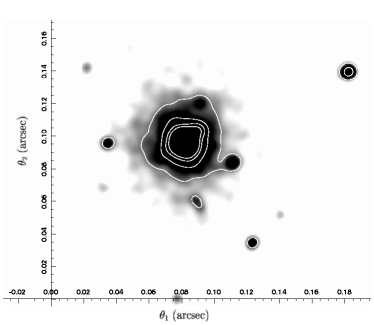
Figure 1: The cut-out of the surface mass density map of the simulated galaxy. The mass distribution resulting from the cosmological N-body simulation (see text) was smoothed using convolution with a Gaussian kernel characterised by a standard deviation $\sigma\sim 0.8\;{\rm kpc}\sim 0.2\>{\rm arcsec}$. This map was then evaluated on $2048\>\times\>2048$ grid points ($\sim 160\>\times\;160\>{\rm kpc}$) and the surface mass density was calculated. Test particles, used in the N-body simulation to account for the large-scale structure, have been removed here. The contours correspond to the values of $\kappa=0.8;1.6;2.4;3.2$. The dark regions represent the regions of high $\kappa$. The units on the axes are arcseconds; one arcsecond in the lens plane corresponds to approximately $4\>{\rm kpc}$.

The simulations were performed using GRAPESPH, a code that combines the hardware N-body integrator GRAPE with the Smooth Particle Hydrodynamics technique (Steinmetz 1996). GRAPESPH is fully Lagrangian and optimally suited to study the formation of highly non-linear systems in a cosmological context. The version used here includes the self-gravity of gas, stars, and dark matter components, a three-dimensional treatment of the hydrodynamics of the gas, Compton and radiative cooling (assuming primordial abundances), the effects of a photo-ionizing UV background, and a simple recipe for transforming gas into stars.

The original simulated field is located at $z=0.2$ and contains approximately 300000 particles. The simulation is contained within a sphere of diameter $32\;{\rm Mpc}$ which is split into a high resolution sphere of diameter $2.5\;{\rm Mpc}$ centred around a galaxy and an outer low resolution shell. Gas dynamics and star formation is restricted to the high resolution sphere (280000 particles, 92000 of which dark matter), while the 34000 dark matter particles of the low resolution sphere sample the large scale matter distribution in order to appropriately reproduce the large scale tidal fields (see Navarro & Steinmetz 1997 and Steinmetz & Navarro 2000 for details on this simulation technique).

The simulation was performed in a $\Lambda$CDM cosmology ($\Omega_{0}=0.3$, $\Omega_{\Lambda}=0.7$, $\Omega_{\rm b}=0.019/h^{2}$, $\sigma_{8}=0.9$). It has a mass resolution of $1.26\times 10^{7}M_{\odot}$ and a spatial resolution of $0.5\>{\rm kpc}$. A realistic resolution scale for an identified substructure is typically assumed to be $\sim 40$ particles which corresponds to $5\times 10^{8}M_{\odot}$. The quoted mass resolution holds for gas/stars. The high resolution dark matter particles are about a factor of 6 ($=\Omega_{0}/\Omega_{\rm b}$) more massive.

From the original simulated field we took a cut-out map of size $\sim 160\>\times\;160\>{\rm kpc}$ that is centred on a single galaxy. This area lies well within the high resolution sphere and is void of any massive intruder particles from the low resolution shell. The resulting mass distribution was smoothed using convolution with a Gaussian kernel characterised by a standard deviation of $\sigma\sim 0.8\>{\rm kpc}\sim 0.2\>{\rm arcsec}$. This map was then evaluated on $2048\;\times\;2048$ grid points. The final map contains information about approximately 130000 particles with a total mass of $3.0\times 10^{12}\;{\rm M_{\odot}}$. The surface mass density $\kappa$ was calculated for every grid point. We chose the redshift of the source to be $z=3$. A part of the cut-out map can be seen in Fig. 1.

The lens properties are calculated on a grid of $2048\>\times\>2048$ points. The Poisson equation

$$\nabla^{2}\psi(\mathchoice{\mbox{\boldmath$\displaystyle\theta$}}{\mbox{\boldmath$\textstyle\theta$}}{\mbox{\boldmath$\scriptstyle\theta$}}{\mbox{\boldmath$\scriptscriptstyle\theta$}})=2\,\kappa(\mathchoice{\mbox{\boldmath$\displaystyle\theta$}}{\mbox{\boldmath$\textstyle\theta$}}{\mbox{\boldmath$\scriptstyle\theta$}}{\mbox{\boldmath$\scriptscriptstyle\theta$}})\;.$$ (10)

is solved (on the grid) in Fourier space by the FFT (Fast Fourier Transformation) method. This method is incorporated in the routine KAPPA2STUFF from the IMCAT software of Nick Kaiser (http://www.ifa.hawaii.edu/~kaiser) that we used. It takes a grid map of $\kappa(\mathchoice{\mbox{\boldmath$\displaystyle\theta$}}{\mbox{\boldmath$\textstyle\theta$}}{\mbox{\boldmath$\scriptstyle\theta$}}{\mbox{\boldmath$\scriptscriptstyle\theta$}}_{j})$ as an input and returns the values of deflection angle and complex shear (in x-space), along with other quantities. From these data we calculated the Jacobi matrix for each grid point.

The simulated galaxy is a field galaxy. Therefore we add two external shear components to the Jacobi matrix (evaluated at each grid point) in order to make it similar to the galaxy in B1422+231. The shear components were taken to be the same as the ones obtained from the best fitting SIE+SH model

$$\gamma_{1}^{\rm ext}=-0.04\;,\quad\gamma_{2}^{\rm ext}=-0.16\;.$$

The external shear accounts for the effect of the neighbouring galaxies of the compact group, which are not present in the simulation.

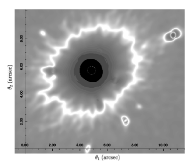
Figure 2: The magnification map of the simulated galaxy calculated using the KAPPA2STUFF routine from Nick Kaiser’s software IMCAT. External shear is added in the evaluation of the magnification map for to account for neighbouring galaxies (see text). Lighter regions represent high magnifications. The units on the axes are arcseconds; one arcsecond in the lens plane corresponds to approximately $4\>{\rm kpc}$.

Fig. 2 shows the magnification map of the surface mass density (given in Fig. 1) with additional external shear. One can clearly see the outer critical curve (white curve), while only the traces of the inner critical curve are visible (little circle inside the black region). The reason why we can see the outer critical curve so much better than the inner one is the following. At the centre $\mathchoice{\mbox{\boldmath$\displaystyle\theta$}}{\mbox{\boldmath$\textstyle\theta$}}{\mbox{\boldmath$\scriptstyle\theta$}}{\mbox{\boldmath$\scriptscriptstyle\theta$}}_{\rm c}$ of the galaxy, the surface mass density is very high and the determinant of the Jacobi matrix can be approximated by $\det A\sim\kappa(\mathchoice{\mbox{\boldmath$\displaystyle\theta$}}{\mbox{\boldmath$\textstyle\theta$}}{\mbox{\boldmath$\scriptstyle\theta$}}{\mbox{\boldmath$\scriptscriptstyle\theta$}}_{\rm c})^{2}$. In our particular case, $\kappa(\mathchoice{\mbox{\boldmath$\displaystyle\theta$}}{\mbox{\boldmath$\textstyle\theta$}}{\mbox{\boldmath$\scriptstyle\theta$}}{\mbox{\boldmath$\scriptscriptstyle\theta$}}_{\rm c})\approx 50$, and since at the critical curve $\det A=0$, we see that the determinant has to decrease from 2500 to 0 in a region of $0.4\;{\rm arcsec}$. The transition is therefore very steep and we have a very good chance to miss the maximum value of magnification there, since the resolution is not high enough. At the outer critical curve, the change is slower and we can clearly see the points of high magnification.

In order to generate a similar image configuration as the one in B1422+231, one considers the caustic curve. This can be done by simply mapping the points of high magnification onto the source plane. Such a map is presented in Fig. 3.

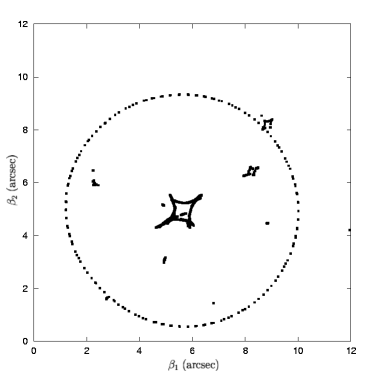
Figure 3: The caustic obtained by mapping the points of high magnification onto the source plane. We took $\left|\mu\right|>30$ for the inner caustic, for the outer one we additionally picked the points of $\left|\mu\right|>0.5$ (due to nummerical effects – see text) from the central part of the magnification map. The units on the axes are arcseconds; one arcsecond in the source plane corresponds to approximately $6\>{\rm kpc}$ for the source at $z=3$.

On first sight the caustic structure of the N-body simulated galaxy looks the same as e.g. the caustic of the smooth NIE model with a small core radius. However, if we look only at the inner, asteroid caustic we can see that it is not completely “smooth”. With the help of bilinear interpolation we recalculated the magnification map on a refined grid (increasing the number of points being evaluated by $5\>\times 5$) and the corresponding caustic for such a grid is shown in Fig. 4. The caustic structure is much more complicated than in the case of a smooth model; in addition to folds and cusps we also have swallowtails formed (see Schneider et al. 1992 for more details on catastrophe theory).

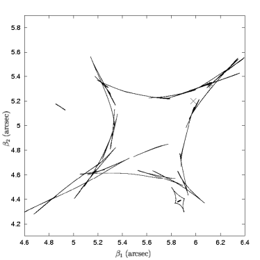
Figure 4: The caustic curves obtained by first interpolating the magnification map on a refined grid using bilinear interpolation (increasing the number of points in the region of interest by a factor of 25) and mapping the points of high magnification $\left|\mu\right|>30$ (Fig. 2) to the source plane. The units on the axes are arcseconds; one arcsecond in the source plane corresponds to approximately $6\>{\rm kpc}$ for the source at $z=3$. Two marks correspond to the source position of data set 1 (cross) and 11 (star) – see Sect. 6.1. The source positions of other data sets are located on a line connecting them.

6.1 Generating synthetic data

We select a source position $\mathchoice{\mbox{\boldmath$\displaystyle\beta$}}{\mbox{\boldmath$\textstyle\beta$}}{\mbox{\boldmath$\scriptstyle\beta$}}{\mbox{\boldmath$\scriptscriptstyle\beta$}}_{\rm s}$ such as to lie inside the asteroid caustic and close to the cusp, trying to chose a position for which we would get similar flux ratios as in the case of B1422+231. In total we considered 11 different source positions (see Fig. 4).

For each of them we first determine approximate image positions using the method described in Sect. 5.1. In order to get exact image positions we use the root finding method MNEWT again, for which we need the deflection angle to be continuous inside the region where we look for images. In our case the deflection angle is defined only on a $2048\times 2048$ grid. We perform bilinear interpolation between grid points. Having the image positions, we performed bilinear interpolation of the magnification map in order to get more exact magnification factors.

6.2 Fitting the synthetic data

For the $\chi^{2}$-fitting method according to (7) we need to determine the uncertainty on the image positions and fluxes. Since we use interpolation for the MNEWT method we do not have a real estimate for the errors. One can, for example, set the errors to the same (relative) values as the uncertainties on the observed radio positions in B1422+231. For the typical scales we are using here (i.e. the distance B to D is approximately $3.5\;{\rm arcsec}$) this would mean an uncertainty of much less than a distance between two grid points. However, such a small error estimate is not realistic; due to the finite grid we estimate the image position uncertainties to be the distance between two grid points (which is a generous estimate; we use bilinear interpolation so the uncertainty is probably lower). The flux ratio errors were then set to be approximately 2 % for images A, B and C and 5 % for image D. These uncertainties are set to be the same as in the case of observed radio fluxes in B1422+231. The galaxy position error is set twice as big as that for the image positions.

The fitting procedure is performed in the same way as for the B1422+231 data. Again, image B is taken as a reference and the $\chi^{2}$-function is evaluated according to (7). We try to fit the positions and fluxes with SIE+SH and SIE+SH+NIS models. The flux ratios of the 11 sets of synthetic data, together with the results of the minimisation are presented in table 7. We experience similar problems fitting fluxes as before; the $\chi^{2}$-function value is high for all 11 data sets.

What might be surprising is the fact that we do not recover some properties of the lensing system. We know that the primary lens is fairly circular (one can not see that from fig. 2, since there, external shear is already added) and we know the values of the external shear components. What we also know a priori are the magnification factors for the images. These values were not recovered with high accuracy in model fitting.

Table 7: The flux ratios of image A, C and D w.r.t. image B of 11 data sets with different image positions $\mathchoice{\mbox{\boldmath$\displaystyle\beta$}}{\mbox{\boldmath$\textstyle\beta$}}{\mbox{\boldmath$\scriptstyle\beta$}}{\mbox{\boldmath$\scriptscriptstyle\beta$}}_{\rm s}$ (see also Fig. 4). Listed are also the resulting $\chi^{2}$ values for fitting image positions and fluxes with SIE+SH model ($\chi^{2}_{1}$) and SIE+SH+NIS model ($\chi^{2}_{2}$). The core radius and $\sigma_{\rm NIS}$ of the perturbing galaxy were fixed to the values $\theta_{\rm c}=1\;{\rm mas}$ and $\sigma_{\rm NIS}=15\;{\rm km/s}$.

Data set	$F_{\rm AB}$	$F_{\rm CB}$	$F_{\rm DB}$	$\chi_{1}^{2}$	$\chi_{2}^{2}$
1	1.04	0.80	0.220	120	2.0
2	1.29	1.20	0.193	960	120
3	1.43	1.40	0.167	2100	190
4	1.20	0.79	0.142	660	5.1
5	1.06	0.59	0.116	350	3.9
6	1.05	0.42	0.089	150	81
7	1.06	0.31	0.064	450	110
8	0.60	0.29	0.047	93	40
9	0.51	0.46	0.051	400	180
10	0.59	0.52	0.064	86	9.3
11	0.62	0.66	0.070	240	36

For a smooth model and a source close to the cusp, the flux relation described before holds. We see that the fluxes violate this rule in all configurations we used. As we mentioned before this relation can only be violated when the source is away from the cusp or if there is substructure in the system. Since here we know the source position, the N-body lensing results show that the substructure we have in this particular simulated galaxy is indeed responsible for the observed deviation.

6.3 Discussion of the results from N-body lensing

An important question is whether the N-body simulation galaxy we are using is a good representation of a real galaxy for the purpose of lensing. If the resolution is not high enough, an N-body simulated galaxy might show more substructure than a real galaxy has.

In order to obtain the surface mass density map representative of lensing and to try to make sure that the substructure we see is not of numerical origin we used a smoothing length for particles of $\sigma=0.8\>{\rm kpc}\sim 0.2\>{\rm arcsec}$. The individual mass clumps we see in the corresponding surface mass density map (Fig. 1) therefore contain well above 100 particles. As we mentioned before, a realistic resolution scale for an identified substructure in the simulation corresponds to $\sim 40$ particles.

The regions that are interesting for multiple image formation typically have $\kappa$ values of order unity. In such regions we have approximately 300 particles per smoothing area, which, if the noise were Poissonian, would result in an error of about $1/\sqrt{N}\sim 0.06$. However, studies of errors of N-body simulations using smoothed particle hydrodynamics (Monaghan 1992; Niedereiter 1978) show that the errors are significantly smaller, and behave as $\propto\log N/N$.

Any deviation of $\kappa$ due to substructure larger than the estimated error of the N-body simulations tells us that we are dealing with “physical” substructure, i.e. not of numerical origin. Our surface mass density maps show deviations well above the estimated Poisson noise, and therefore also above numerical noise. The results shown in Table 7 are affected by the “physical” substructure as well as by the noise. Although the expected noise is significantly smaller than believable substructure observed in the N-body simulations, it is hard to precisely estimate the relative contributions in the results shown here.

There are indications that the level of substructure as obtained from simulations can influence lensing phenomena a lot. In particular, the synthetic fluxes we obtained deviate strongly from those predicted by smooth models. This particular example of a simulated galaxy can of course not give us the answers to the aforementioned questions. In order to draw stronger conclusions, one would have to investigate many different realisations of N-body simulated galaxies and in addition use higher resolution simulations (currently unavailable). A statistical analysis to investigate the strong lensing properties could then be made. This is, however, beyond the scope of this paper and will be considered in a future work.

7 Conclusion

In this work we have investigated the influence of substructure in the gravitationally lensed system B1422+231. While it is intuitively clear that a lens galaxy is not a smooth entity, we have tried to investigate how deviation from a smooth model can influence lensing phenomena, especially the image flux ratios.

We have used two different smooth models for the lensing galaxy (SIE+SH and NIE+SH), and both failed very badly in fitting the image fluxes (we got $\chi^{2}=130$ with 2 degrees of freedom). The use of models with substructure requires additional observational constraints. Therefore, we used deconvolved image shapes as constraints. We get a significant improvement of the fit compared to the smooth model. However, the way the substructure is introduced is oversimplified, thus we should not be surprised that the resulting $\chi^{2}$ is still high. For the model with a single perturber we got $\chi^{2}=19$ for 6 degrees of freedom, and with two perturbers we had $\chi^{2}=15$ for 4, while the model without substructure (where deconvolved image shapes were included) gives $\chi^{2}=140$ for 8 degrees of freedom.

Up to now we have not considered the possibility that microlensing plays a role for the radio fluxes. Koopmans & de Bruyn (2000) claim that they have detected microlensing in the multiply-imaged radio source B1600+434. Microlensing is a very tempting explanation for difficulties in fitting the fluxes for it can also explain why the $8.4\>{\rm GHz}$ A:B flux ratio has changed from 0.97 in 1991 (Patnaik et al. 1992) to 0.93 in 1997 (Patnaik et al. 1999). This has a consequence that again speaks in favour of substructure, since the presence of radio microlensing indicates that there is a significant number of compact objects in the lens galaxy halo.

N-body simulation data of a model galaxy provides a test for the influence of mass-substructure in strong gravitational lensing. When we generated data of four image systems with the simulated galaxy we again experienced difficulties. We have tried to fit image positions and fluxes and failed to obtaining a model that fits well. From these experiments we can conclude that the level of substructure obtained from this particular N-body simulated galaxy can cause the same difficulties as experienced in some of the real gravitationally lensed systems.

In order to obtain stronger conclusions one would have to investigate more realisations of simulated galaxies, also at different redshifts. However, the N-body simulation results indicate that substructure plays an important role in strong lensing. Also, modelling B1422+231 shows that the fluxes of more than one image are probably affected by the lens substructure. With the conclusions one can draw from lens modelling we can not give a direct answer about the properties of mass substructure in B1422+231.

One should therefore avoid using the flux constraints directly; they should, rather, be treated in statistical manner, e.g. in a way suggested by Mao & Schneider (1998). Fortunately, the perturbations on the scales we are dealing with here do not influence the image positions significantly, and play even less of a role for the time delay (Mao & Schneider 1998). Strong lensing thus remains one of the best tools to constrain the Hubble constant.