Neutrino production in a time-dependent matter background

Marieke Postma

Department of Physics and Astronomy, UCLA, Los Angeles, CA 90095-1547

We show that neutrinos can be produced through standard electroweak interactions in matter with time-dependent density.

PRESENTED AT

COSMO-01
Rovaniemi, Finland,
August 29 – September 4, 2001

1 Introduction

In this talk I will show that neutrinos can be pair produced by a time-dependent matter density through standard electroweak interactions. The idea is that both ordinary matter and the nuclear matter found in neutron stars carry a net SU(2) charge. Neutrinos couple to this charge through the electroweak interactions. In a time-dependent matter background this leads to neutrino pair production [1]. This phenomenon is analagous to electron pair production by a time-varying electromagnetic field [2, 3], or fermion production by a variable scalar field as can occur during preheating [4, 5]. Applications include density waves in a neutron star, a neutron star in a binary system, or a supernova explosion. We expect the amount of neutrinos produced to be small though.

2 Formalism

The starting point in our description of neutrino production is the Dirac equation for a neutrino in the presence of a time-dependent electroweak current $j^{\mu}(t)$:

$$\left[i\gamma^{0}\partial_{0}+i\gamma^{k}\partial_{k}+j_{\mu}(t)\gamma^{\mu}P_{\rm L}-m\right]\psi=0.$$ (1)

Here $P_{\rm L}$ is the projection operator on left handed states. In electrically neutral matter, the isospin of protons and electrons cancel, and the net weak current is proportional to the number density of neutrons $n_{n}$. Let us consider the case of a spatially uniform matter density moving with a four-velocity $v_{\mu}$. Then $j_{\mu}=\rho v_{\mu}$ with $\rho=(G_{F}/\sqrt{2})n_{n}$. The largest values of the “reduced density” $\rho$ are obtained in nuclear matter. In a neutron star the reduced density ranges from $\rho\sim 10^{3}\,{\rm eV}$ in core to $\rho\sim 10^{-3}\,{\rm eV}$ in the outer layers.

To solve the Dirac equation it proves convenient to rewrite it as a second order differential equation for scalar functions. To do so we expand the neutrino field in a complete set of eigenmodes

$$\psi=\sum_{s=\pm}\int\frac{d^{3}k}{(2\pi)^{3}}\left[b_{{\bf k},s}U_{{\bf k},s}(t)+d_{-{\bf k},s}^{{\dagger}}V_{-{\bf k},s}(t)\right]e^{i{\bf k}{\bf x}}.$$ (2)

For the eigenspinors we make the following Ansatz

$$U_{{\bf k},s}(t)e^{i{\bf k}{\bf x}} = N_{{k},s}\left[i\gamma^{\mu}\partial_{\mu}+m+j_{\mu}(t)\gamma^{\mu}P_{\rm L}\right]\phi^{(1)}_{k,s}(t)R_{k,s}^{(1)}{\rm e}^{i{\bf k}{\bf x}-\i/2\int_{0}^{t}\rho_{\pm}(\zeta)d\zeta},$$

$$V_{{\bf-k},s}(t)e^{i{\bf k}{\bf x}} = N_{{k},s}\left[i\gamma^{\mu}\partial_{\mu}+m+j_{\mu}(t)\gamma^{\mu}P_{\rm L}\right]\phi^{(-1)}_{k,s}(t)R_{k,s}^{(-1)}{\rm e}^{i{\bf k}{\bf x}-\i/2\int_{0}^{t}\rho_{\pm}(\zeta)d\zeta}.$$ (3)

$N_{{k},s}$ are normalization constants. We choose the time-independent spinors $R_{k,s}^{(\lambda)}$, $\lambda=\pm 1$, such that they transform into each other under the action of $\gamma^{0}$, and that they are eigenvectors of the spin operator:

$$\gamma^{0}R_{k,s}^{(\lambda)}=R_{k,s}^{(-\lambda)},\qquad\gamma^{0}\vec{\gamma}\cdot\vec{k}R_{k,\pm}^{(\lambda)}=\pm R_{k,\pm}^{(\lambda)}.$$ (4)

This latter property means that for matter moving with some velocity, we choose $\vec{v}\parallel\vec{k}$. We do not expect the orthogonal momenta to change the overall picture of particle production. Substituting this Ansatz back in the Dirac equations gives the desired equation for the mode functions $\phi^{(\lambda)}_{k,s}$:

$$\ddot{\phi}_{k,\pm}^{(\lambda)}+\left[m^{2}+k_{\rm eff,\pm}^{2}-i\frac{\lambda}{2}\dot{\rho}_{\pm}\right]\phi_{k,\pm}^{(\lambda)}=0,$$ (5)

where we have aligned the neutrino momentum and the velocity of the background matter with the $3$rd axis, and we introduced the shorthand notation $\rho_{\pm}=\rho_{0}(v_{0}\pm v_{3})$. Furthermore $k_{\rm eff,\pm}(t)=\pm k+\rho_{\pm}(t)/2$ is the time-dependent effective neutrino momentum. The shift in momentum is due to the presence of the electroweak potential generated by the matter background.

The solutions corresponding to the two values of $\lambda$ satisfy equations that are complex conjugate of each other, i.e.,

$$\left(\phi_{k,\pm}^{(\lambda)}\right)^{*}=\phi_{k,\pm}^{(-\lambda)}.$$ (6)

Hence, these functions are related by charge conjugation, and thus the spinors $U$ and $V$ correspond to particle and anti-particle states. In the presence of a matter background the charge conjugation symmetry C is spontaneously broken. The time-dependent phase factor in eq. (3) is introduced to restore this symmetry for the mode functions $\phi^{(\lambda)}_{k,\pm}$; under charge conjugation the sign of the momentum and of the reduced density $\rho$ are changed similtanuously.

We choose initial conditions at $t\leq 0$ corresponding to a constant matter background. The mode functions are then simply plane wave solution with energies that can be read off from the mode equation (5),

$$\phi_{k,\pm}^{(\lambda)}(0)=1,\quad\dot{\phi}_{k,\pm}^{(\lambda)}(0)=\lambda E_{k,\pm}(0)\quad{\rm with}\;E_{k,\pm}(0)=\sqrt{m^{2}+k_{\rm eff,\pm}^{2}(0)}.$$ (7)

In the limit $\rho\to 0$, the spinors $U$ and $V$ become the usual free field positive and negative frequency solutions. We normalize the spinors $U_{{k},r}^{{\dagger}}(0)U_{{k},s}(0)=V_{-{k},r}^{{\dagger}}(0)V_{-{k},s}(0)=\delta_{rs}$. This fixes the normalization constant in eq. (3), $N_{k,\pm}^{-2}=(E_{k,\pm}(0)-k_{\rm eff,\pm}(0))^{2}+m^{2}$. The normalization properties are preserved by the unitary time-evolution of the system.

The system — a neutrino in the presence of weakly charged matter — is solved by solving the mode equations, with given initial conditions and normalization. The next question then is: “What do the solutions mean in terms of particle production?”

3 Particle number

The number operator constructed from the creation and annihilation operators in the mode expansion, eq. (2) is time-independent. Clearly, this will not do to discuss particle production. Particle production is associated with the time-dependence of the Hamiltonian. One can introduce time-dependent creation and annihilation operators that diagonalize the Hamiltonian instantaneously. This defines a physically motivated, time-dependent number operator. Equivalently one can describe particle production in terms of the mode functions. The initial mode functions are positive and negative frequency solutions to the mode equation. However, due to the time-dependence of the Hamiltonian, at later times they will in general be a superposition of positive and negative frequencies, the overlap being a measure of particle production. One finds for the particle number

$${\mathcal{N}}^{P}_{k,s}(t)=|D^{P}_{k,s}|^{2},$$ (8)

where the so-called Bogoliubov coefficient $D^{P}_{k,s}={U_{{\bf k},\pm}}^{{\dagger}}(0)V_{-{\bf k},\pm}(t)$ is (up to a phase)

$$D^{P}_{k,\pm}={m}{N_{{\bf k},\pm}^{2}}\left[i\dot{\phi}^{(-1)}_{k,s}(t)-\phi^{(-1)}_{k,s}(t)\left(E^{(-1)}_{k,\pm}(0)+\frac{1}{2}(\rho_{\pm}(0)-\rho_{\pm}(t))\right)\right].$$ (9)

Both $U$ and $V$ are unitary matrices, and thus the Boguliubov coefficient cannot exceed unity, in accordance with the Pauli exclusion principle. Note further that particle production goes to zero in the limit of a massless neutrino. This is as expected, since in this limit the left and right handed sector decouple, and if the Hamiltonian is diagonal at the initial time, it remains so at all times.

4 Results

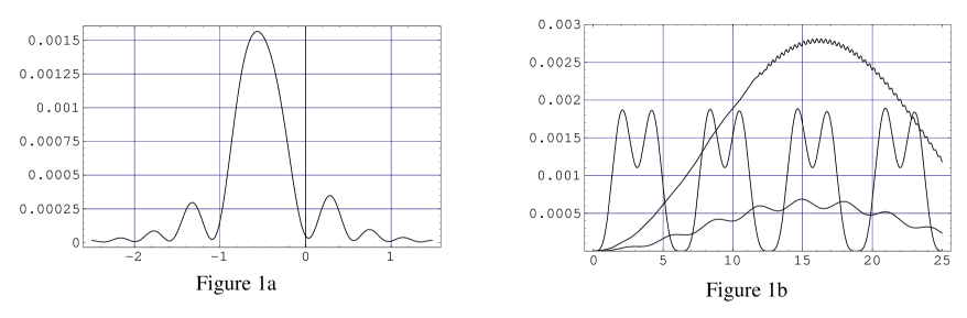
Figure 1: Paricle production in an oscillating matter background $j^{0}=1+0.1\sin(\omega t)$ and $\vec{j}=0$. Fig. 1a shows ${\mathcal{N}}_{{k},+}$ vs. momentum $k$ for $\omega=1$ and time $t=10$. Fig. 1b shows ${\mathcal{N}}_{{k},+}$ as a function of time $t$. The upper curve corresponds to $\!(\omega,k)=(10,4.3)$ (close to resonance), the middle curve to $(\omega,k)=(1,-0.5)$, and the lower curve to $(\omega,k)=(0.1,-0.5)$. All quantities are in units of $m$.

As an explicit example we have calculated numerically the neutrino production in a matter background that is changing periodically with time: $j^{0}=\rho(t)=1+0.1\sin(\omega t)$ and $\vec{j}=0$ (all quantities in units of $m$). The results are shown in figure 1a and b. Figure 1a shows that neutrino production is peaked where the effective momentum $k_{\rm eff}=k+\rho/2$ is zero, and the instantaneous energy appearing in the mode equation (5) is minimized. The width of the excited band is set by the neutrino mass. Figure 1b shows particle number as a function of time. It oscillates, corresponding to creation and annihilation of neutrino pairs. What is left out of the picture is the diffusion of neutrinos as a result of the finite size of the matter region, i.e., neutrinos can escape the production region before they are absorbed. If diffusion is efficient, the production rate is of the order of the slope in fig 1b.

How effective is the neutrino production mechanism? To get an idea, we compare this process with another process in which fermions can be produced, namely preheating. In simple models of inflation the inflaton field $I$ starts oscillates in a potential well at the end of inflation. If the inflaton couples to a fermionic field, this leads to copious production of fermions. Particle production occurs in the non-adiabatic regime, when the inflaton field goes through the minimum of the potential well and $\dot{I}\gg I^{2}$. As a result, the width of the resonance band is set by the frequency of oscillations, which can be much larger than the fermion mass. Furthermore, the dimensionless effective inflaton-fermion coupling $\lambda\sim I_{0}/\omega$ is large because of the large amplitude of oscillation $I_{0}$. Fermion production is unsurpressed, and ${\mathcal{N}}^{P}_{k,s}={\mathcal{O}}(1)$. Neutrino production on the other hand occurs in the adiabatic regime, since for physically realistic values of $\omega$ we have $\dot{\rho}/2\ll E_{\rm ins}^{2}$ at all times (here $E_{\rm ins}=\sqrt{m^{2}+k_{\rm eff}^{2}}$ is the instantaneous energy of the mode functions). The width of the resonance is then set by the neutrino mass, or by the size of the matter perturbation $\delta\rho$ if $m>\delta\rho$; both are at most the order of eV. Moreover the effective dimensionless coupling $\lambda=\delta\rho/m\stackrel{{\scriptstyle<}}{{\sim}}1$, and particle number is surpressed by a factor ${\mathcal{N}}^{P}_{k,s}\propto\lambda^{2}$.

5 Conclusions

To summarize, neutrinos can be pair produced by a time-dependent matter background. Although neat, the phenomenon seems of little practical importance. Due to the smallness of all mass scales involved, the amount of neutrinos produced is small.

ACKNOWLEDGEMENTS

This work was supported in part by the US Department of Energy grant DE-FG03-91ER40662, Task C, as well as by a Faculty Grant from UCLA Council on Research.

References

- [1] A. Kusenko and M. Postma, hep-ph/0107253.
- [2] J. M. Cornwall and G. Tiktopoulos, Phys. Rev. D 39 (1989) 334.
- [3] A. A. Grib, V. M. Mostepanenko, and V. M. Frolov, Theor. Math. Phys. 13, 1207 (1972).
- [4] J. Baacke, K. Heitmann and C. Patzold, Phys. Rev. D 58 (1998) 125013
- [5] P. B. Greene and L. Kofman, Phys. Rev. D 62 (2000) 123516 P. B. Greene and L. Kofman, Phys. Lett. B 448 (1999) 6