Mass Reconstruction with CMB Polarization

Abstract

Weak gravitational lensing by the intervening large-scale structure of the Universe induces high-order correlations in the cosmic microwave background (CMB) temperature and polarization fields. We construct minimum variance estimators of the intervening mass distribution out of the six quadratic combinations of the temperature and polarization fields. Polarization begins to assist in the reconstruction when $E$-mode mapping becomes possible on degree-scale fields, i.e. for an experiment with a noise level of $\sim 40\mu$K-arcmin and beam of $\sim 7^{\prime}$, similar to the Planck experiment; surpasses the temperature reconstruction at $\sim 26\mu$K-arcmin and $4^{\prime}$; yet continues to improve the reconstruction until the lensing $B$-modes are mapped to $l\sim 2000$ at $\sim 0.3\mu$K-arcmin and $3^{\prime}$. Ultimately, the correlation between the $E$ and $B$ modes can provide a high signal-to-noise mass map out to multipoles of $L\sim 1000$, extending the range of temperature-based estimators by nearly an order of magnitude. We outline four applications of mass reconstruction: measurement of the linear power spectrum in projection to the cosmic variance limit out to $L\sim 1000$ (or wavenumbers $0.002\lesssim k\lesssim 0.2$ in $h$/Mpc), cross-correlation with cosmic shear surveys to probe the evolution of structure tomographically, cross-correlation of the mass and temperature maps to probe the dark energy, and the separation of lensing and gravitational wave $B$-modes.

1. Introduction

The weak gravitational lensing of cosmic microwave background (CMB) temperature and polarization anisotropies provides a unique opportunity to map the distribution of matter on large scales and high redshift where density fluctuations were still linear. Although lensing effects are apparent in the power spectra of temperature and polarization (Seljak 1996; Zaldarriaga & Seljak 1998), it is the higher order correlations induced by lensing that make mass reconstruction possible (Bernardeau 1997).

By remapping the CMB fields according to potential gradients, lensing acts as a convolution in Fourier space which introduces correlations between angular wavenumbers or multipole moments. From a quadratic combination of the multipoles, one can form estimators of the potential field and hence the intervening mass. Zaldarriaga & Seljak (1999) and Guzik et al. (2000) constructed noisy estimators out of the product of gradients of the temperature and polarization fields. Hu (2001a,b) showed that the minimum variance estimator constructed from the temperature field has substantially greater signal-to-noise with arcminute resolution CMB maps. This estimator enables mapping of the dark matter above the degree scale, where the deflection power peaks. The cosmic variance of the CMB temperature field itself prevents mapping on smaller scales. In this Paper, we show how this limitation can be overcome with minimum variance quadratic estimators involving the polarization field.

The CMB polarization field in principle provides a more direct probe of lensing than the temperature field. Unlike the temperature anisotropy, there is negligible cosmological contamination of the polarization field in the arcminute regime (Hu 2000a). Furthermore, density perturbations in the linear regime generate only the so-called $E$-mode polarization (Kamionkowski, Kosowsky & Stebbins 1997; Zaldarriaga & Seljak 1997). Lensing converts $E$-mode polarization to its complement, the $B$-mode polarization (Zaldarriaga & Seljak 1998). Although gravitational waves also generate $B$-mode polarization, they do so only above the degree scale. Hu (2000b) and Benabed et al. (2001) used the induced correlation between the $E$ and the $B$-modes to construct statistical measures of the lensing. Here we show that the correlation allows a direct reconstruction of the lensing masses which in fact has in principle the highest signal-to-noise of all the quadratic estimators.

In practice, achieving this potential in the presence of detector noise, systematics and foreground contamination of the polarization will be challenging. These same challenges will also have to be overcome in order to probe the physics of the early universe through gravitational wave $B$-mode polarization. A lensing study can therefore be conducted as secondary science for an experiment devoted to gravitational waves. In fact, as the leading cosmological contaminant of the gravitational wave $B$-modes, a lensing study may well be required of such an experiment (Hu 2001c).

We begin in §2 with a brief review of lensing effects on the temperature and polarization fields. In §3, we present a formal study of the minimum variance quadratic estimators of the lensing potential and show that the $EB$ combination can produce a high signal-to-noise mass map out to the $10^{\prime}$ scale. We explicitly construct this estimator in §4 and simulate its performance in the presence of detector noise. We discuss applications of mass reconstruction in §5. For illustrative purposes, we use a flat $\Lambda$CDM cosmology throughout with parameters $\Omega_{c}=0.3$, $\Omega_{b}=0.05$, $\Omega_{\Lambda}=0.65$, $h=0.65$, $n=1$, $\delta_{H}=4.2\times 10^{-5}$ and no gravitational waves.

   

   

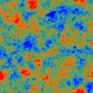
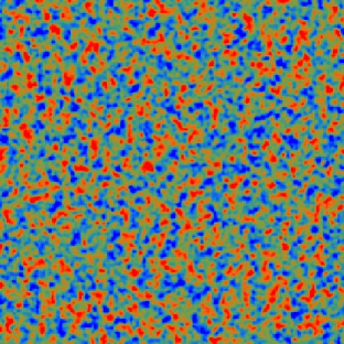
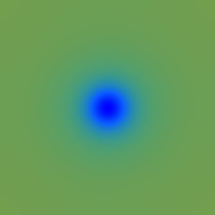
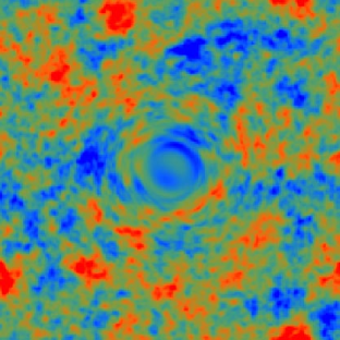
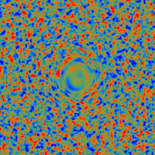
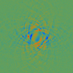
Figure 1.— An exaggerated example of the lensing effect on a $10^{\circ}\times 10^{\circ}$ field. Top: (left-to-right) unlensed temperature field, unlensed $E$-polarization field, spherically symmetric deflection field $d(\bf n)$. Bottom: (left-to-right) lensed temperature field, lensed $E$-polarization field, lensed $B$-polarization field. The scale for the polarization and temperature fields differ by a factor of 10.

2. Lensing

Weak lensing by the large-scale structure of the Universe remaps the primary temperature field $\Theta(\hat{\bf n})=\Delta T(\hat{\bf n})/T$ and dimensionless Stokes parameters $Q(\hat{\bf n})$ and $U(\hat{\bf n})$ as (Blanchard & Schneider 1987; Bernardeau 1997; Zaldarriaga & Seljak 1998)

$$\Theta(\hat{\bf n}) = \tilde{\Theta}(\hat{\bf n}+{\bf d}(\hat{\bf n}))\,,$$ (1)

$$\,[Q\pm iU](\hat{\bf n}) = [\tilde{Q}\pm i\tilde{U}](\hat{\bf n}+{\bf d}(\hat{\bf n}))\,,$$

where $\hat{\bf n}$ is the direction on the sky, tildes denote the unlensed field, and ${\bf d}(\hat{\bf n})$ is the deflection angle. It is related to the line of sight projection of the gravitational potential $\Psi({\bf x},D)$ as ${\bf d}=\nabla\phi$,

$$\phi(\hat{\bf n})=-2\int dD\,{(D_{s}-D)\over D\,D_{s}}\Psi(D\hat{\bf n},D)\,,$$ (2)

where $D$ is the comoving distance along the line of sight in the assumed flat cosmology and $D_{s}$ denotes the distance to the last-scattering surface. In the fiducial cosmology the rms deflection is $2.6^{\prime}$ but its coherence is several degrees.

We will work mainly in harmonic space and consider sufficiently small sections of the sky such that spherical harmonic moments of order $(l,m)$ may be replaced by plane waves of wavevector ${\bf l}$. The all-sky generalization will be presented in a separate work (Okamoto & Hu, in prep). In this case, the temperature, polarization, and potential fields may be decomposed as

$$\Theta(\hat{\bf n}) = \int{d^{2}l\over(2\pi)^{2}}\Theta({\bf l})e^{i{\bf l}\cdot\hat{\bf n}}\,,$$ (3)

$$\,[Q\pm iU](\hat{\bf n}) = -\int{d^{2}l\over(2\pi)^{2}}[E({\bf l})\pm iB({\bf l})]e^{\pm 2i\varphi_{\bf l}}e^{i{\bf l}\cdot\hat{\bf n}}\,,$$

$$\phi(\hat{\bf n}) = \int{d^{2}L\over(2\pi)^{2}}\phi({\bf L})e^{i{\bf L}\cdot\hat{\bf n}}\,,$$

where $\varphi_{{\bf l}}=\cos^{-1}(\hat{\bf x}\cdot\hat{\bf l})$. Lensing changes the Fourier moments by (Hu 2000b)

$$\delta\Theta({\bf l}) = \int{d^{2}l^{\prime}\over(2\pi)^{2}}\tilde{\Theta}({\bf l}^{\prime})W({\bf l}^{\prime},{\bf L})\,,$$ (4)

$$\delta E({\bf l}) = \int{d^{2}l^{\prime}\over(2\pi)^{2}}\Big{[}\tilde{E}({\bf l}^{\prime})\cos 2\varphi_{{\bf l}^{\prime}{\bf l}}-\tilde{B}({\bf l}^{\prime})\sin 2\varphi_{{\bf l}^{\prime}{\bf l}}\Big{]}W({\bf l}^{\prime},{\bf L})\,,$$

$$\delta B({\bf l}) = \int{d^{2}l^{\prime}\over(2\pi)^{2}}\Big{[}\tilde{B}({\bf l}^{\prime})\cos 2\varphi_{{\bf l}^{\prime}{\bf l}}+\tilde{E}({\bf l}^{\prime})\sin 2\varphi_{{\bf l}^{\prime}{\bf l}}\Big{]}W({\bf l}^{\prime},{\bf L})\,,$$

where $\varphi_{{\bf l}^{\prime}{\bf l}}\equiv\varphi_{{\bf l}^{\prime}}-\varphi_{{\bf l}}$, ${\bf L}={\bf l}-{\bf l}^{\prime}$, and

$$W({\bf l},{\bf L})=-[{{\bf l}\cdot{\bf L}}]\phi({\bf L})\,.$$ (5)

Here $\delta\Theta=\Theta-\tilde{\Theta}$ for example. In Fig. 1, we show a toy example of the effect of lensing on the temperature and polarization fields (see also Benabed et al. 2001). The effect on the $E$-polarization is similar to that of the temperature and reflects the fact that $\cos 2\varphi_{{\bf l}^{\prime}{\bf l}}\approx 1$ for $L\ll l$, where the lens is smooth compared with the field. Even in the absense of an unlensed $B$-polarization, lensing will generate it. The lensing structure differs since $\sin 2\varphi_{{\bf l}^{\prime}{\bf l}}\approx 0$ for $L\ll l$. This fact will ultimately lead to a different range in $L$ of sensitivity to $\phi$ from the various fields.

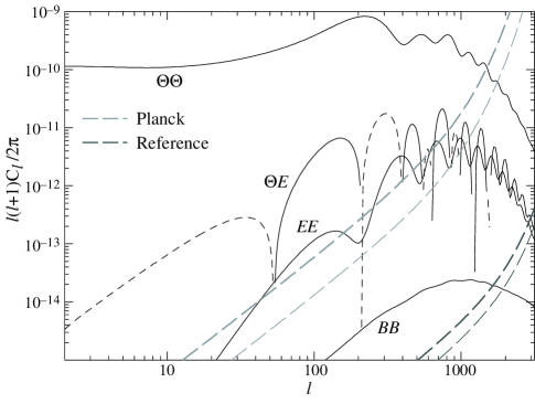
Figure 2.— Power spectra of the CMB temperature and polarization fields compared with the detector noise of the Planck satellite and a nearly perfect experiment with a noise level of $\Delta_{T}=\Delta_{P}/\sqrt{2}=1\mu$K-arcmin and a beam of $\sigma=4^{\prime}$ (long dashed lines, thick for polarization, thin for temperature). The Planck experiment has sufficient signal-to-noise to map the $\Theta$ field but can only marginally map the $E$-polarization field; the nearly perfect experiment can map the all three fields to $l=2000$.

Since the unlensed fields and potential perturbations are assumed to be Gaussian and statistically isotropic, the statistical properties of the lensed fields may be completely defined by the unlensed power spectra

$$\langle\tilde{x}^{*}({\bf l})\tilde{x}({\bf l}^{\prime})\rangle \equiv (2\pi)^{2}\delta({\bf l}-{\bf l}^{\prime})\tilde{C}_{l}^{xx^{\prime}}\,,$$

$$\langle\phi^{*}({\bf L})\phi({\bf L}^{\prime})\rangle \equiv (2\pi)^{2}\delta({\bf L}-{\bf L}^{\prime})L^{-2}C_{L}^{dd}\,,$$

where $x=\Theta$, $E$, $B$ and we have chosen to express the potential power spectrum with a weighting appropriate for the deflection field $d(\hat{\bf n})$. Under the assumption of parity invariance

$$\tilde{C}_{l}^{\Theta B}=\tilde{C}_{l}^{EB}=0\,,$$ (6)

and in the absence of gravitational waves and vorticity $\tilde{C}_{l}^{BB}=0$. The peak in the logarithmic power spectrum $L^{2}C_{L}^{dd}/2\pi$ at $L\sim 30-40$ defines the degree-scale coherence of the deflection angles.

Finally, we define the power spectra of the observed temperature and polarization fields as

$$\langle x^{*}({\bf l})x({\bf l}^{\prime})\rangle\equiv(2\pi)^{2}\delta({\bf l}-{\bf l}^{\prime})C_{l}^{xx^{\prime}}\,,$$

where the power spectra include all sources of variance to the fields including detector noise and residual foreground contamination added in quadrature. We will include Gaussian random detector noise of the form (Knox 1995)

$$C_{l}^{\Theta\Theta}\Big{|}_{\rm noise} = \left({\Delta_{T}\over T_{\rm CMB}}\right)^{2}e^{l(l+1)\sigma^{2}/8\ln 2}\,,$$

$$C_{l}^{EE}\Big{|}_{\rm noise}=C_{l}^{BB}\Big{|}_{\rm noise} = \left({\Delta_{P}\over T_{\rm CMB}}\right)^{2}e^{l(l+1)\sigma^{2}/8\ln 2}\,,$$ (7)

where $\Delta_{T,P}$ parameterizes white detector noise, here in units of $\mu$K-radian, $T_{\rm CMB}=2.728\times 10^{6}\,\mu$K, and $\sigma$ is the FWHM of the beam. We will often assume $\Delta_{P}=\sqrt{2}\Delta_{T}$ as appropriate for fully-polarized detectors. In Fig. 2, we compare the signal and noise contributions to the total power spectra for the Planck satellite experiment (minimum variance channel weighting from Cooray & Hu 2000; $\Delta_{T}\approx 27\mu$K-arcmin, $\Delta_{P}\approx 40\sqrt{2}\,\mu$K-arcmin, $\sigma\approx 7^{\prime}$) and a near perfect reference experiment ($\Delta_{T}=\Delta_{P}/\sqrt{2}=1\mu$K-arcmin and $\sigma=4^{\prime}$). In general where the signal exceeds the noise power spectrum of a field, there is sufficient signal-to-noise for mapping. When this is not the case, a statistical detection of the signal may still be possible. The Planck experiment is on the threshold of being able to map the $E$-polarization. The reference experiment can map all 3 fields to $l\sim 2000$.

3. Minimum Variance Estimators

As can be seen from Eqn. (2), lensing mixes and therefore correlates the Fourier modes across a range defined by the power in the deflection field $C_{L}^{dd}$ (Hu 2000b). Consider averaging over an ensemble of realizations of the temperature and polarization fields but with a fixed lensing field. The two-point correlation of the modes takes the form

$$\langle x({\bf l})x^{\prime}({\bf l}^{\prime})\rangle_{\rm CMB}=f_{\alpha}({\bf l},{\bf l}^{\prime})\phi({{\bf L}})\,,$$ (8)

where $x,x^{\prime}=\Theta,E,B$, and ${\bf L}={\bf l}+{\bf l}^{\prime}$. We have assumed ${\bf l}\neq-{\bf l}^{\prime}$ and will use the subscript $\alpha$ to distinguish between choices of the $xx^{\prime}$ pairing, e.g. $\alpha=\Theta\Theta$. The correlation returns the value of the deflection potential with weightings $f_{\alpha}$ that depend on the unlensed power spectra of Eqn. (2), which are given explicitly in Tab. 1.

$\alpha$	$f_{\alpha}({{\bf l}_{1},{\bf l}_{2}})$ [
$\Theta\Theta$	$\tilde{C}_{l_{1}}^{\Theta\Theta}({{\bf L}}\cdot{\bf l}_{1})+\tilde{C}_{l_{2}}^{\Theta\Theta}({{\bf L}}\cdot{\bf l}_{2})$[
$\Theta E$	$\tilde{C}_{l_{1}}^{\Theta E}\cos\varphi_{{\bf l}_{1}{\bf l}_{2}}({{\bf L}}\cdot{\bf l}_{1})+\tilde{C}_{l_{2}}^{\Theta E}({{\bf L}}\cdot{\bf l}_{2})$[
$\Theta B$	$\tilde{C}_{l_{1}}^{\Theta E}\sin 2\varphi_{{\bf l}_{1}{\bf l}_{2}}({{\bf L}}\cdot{\bf l}_{1})$[
$EE$	$[\tilde{C}_{l_{1}}^{EE}({{\bf L}}\cdot{\bf l}_{1})+\tilde{C}_{l_{2}}^{EE}({{\bf L}}\cdot{\bf l}_{2})]\cos 2\varphi_{{\bf l}_{1}{\bf l}_{2}}$ [
$EB$	$[\tilde{C}_{l_{1}}^{EE}({{\bf L}}\cdot{\bf l}_{1})-\tilde{C}_{l_{2}}^{BB}({{\bf L}}\cdot{\bf l}_{2})]\sin 2\varphi_{{\bf l}_{1}{\bf l}_{2}}$ [
$BB$	$[\tilde{C}_{l_{1}}^{BB}({{\bf L}}\cdot{\bf l}_{1})+\tilde{C}_{l_{2}}^{BB}({{\bf L}}\cdot{\bf l}_{2})]\cos 2\varphi_{{\bf l}_{1}{\bf l}_{2}}$ [

Table 1Minimum variance filters

The two point correlations of the CMB Fourier modes themselves cannot be used to reconstruct the deflection potential since $\phi$ is also statistically isotropic so that in the true ensemble average $\langle\phi(L)\rangle=0$. Eqn. (8) does suggest however that an appropriate average over pairs of multipole moments can be used to estimate the deflection field $d({\hat{\bf n}})$.

Let us define a general weighting of the moments

$$d_{\alpha}({{\bf L}})={A_{\alpha}(L)\over L}\int{d^{2}l_{1}\over(2\pi)^{2}}x({\bf l}_{1})x^{\prime}({\bf l}_{2})F_{\alpha}({\bf l}_{1},{\bf l}_{2})\,,$$ (9)

where ${\bf l}_{2}={\bf L}-{\bf l}_{1}$ and the normalization

$$A_{\alpha}(L)=L^{2}\Bigg{[}\int{d^{2}l_{1}\over(2\pi)^{2}}f_{\alpha}({\bf l}_{1},{\bf l}_{2})F_{\alpha}({\bf l}_{1},{\bf l}_{2})\Bigg{]}^{-1}\,.$$ (10)

is chosen so that

$$\langle d_{\alpha}({\bf L})\rangle_{\rm CMB}=d({{\bf L}})\equiv L\phi({{\bf L}})\,.$$ (11)

In general there are 6 estimators corresponding to the $3!$ pairs of $\Theta$, $E$, $B$. In the assumed cosmology, where gravitational wave perturbations are negligible compared with density perturbations, $\alpha=BB$ has vanishing signal-to-noise effectively reducing the estimators to 5.

We can optimize the filter $F_{\alpha}$ by minimizing the variance $\langle d_{\alpha}^{*}(L)d_{\alpha}(L)\rangle$, subject to the normalization constraint

$$F_{\alpha}({\bf l}_{1},{\bf l}_{2})={C_{l_{1}}^{x^{\prime}x^{\prime}}C_{l_{2}}^{xx}f_{\alpha}({\bf l}_{1},{\bf l}_{2})-C_{l_{1}}^{xx^{\prime}}C_{l_{2}}^{xx^{\prime}}f_{\alpha}({\bf l}_{2},{\bf l}_{1})\over C_{l_{1}}^{xx}C_{l_{2}}^{x^{\prime}x^{\prime}}C_{l_{1}}^{x^{\prime}x^{\prime}}C_{l_{2}}^{xx}-(C_{l_{1}}^{xx^{\prime}}C_{l_{2}}^{xx^{\prime}})^{2}}\,.$$ (12)

This filter takes on simple forms for two common cases: if $x=x^{\prime}$, as in the case of $\alpha=\Theta\Theta$, $EE$ and $BB$,

$$F_{\alpha}({\bf l}_{1},{\bf l}_{2})\rightarrow{f_{\alpha}({\bf l}_{1},{\bf l}_{2})\over 2C_{l_{1}}^{xx}C_{l_{2}}^{xx}};$$ (13)

if $\tilde{C}_{l}^{xx^{\prime}}=0$, as in the case of $\alpha=\Theta B$ and $EB$,

$$F_{\alpha}({\bf l}_{1},{\bf l}_{2})\rightarrow{f_{\alpha}({\bf l}_{1},{\bf l}_{2})\over C_{l_{1}}^{xx}C_{l_{2}}^{x^{\prime}x^{\prime}}}.$$ (14)

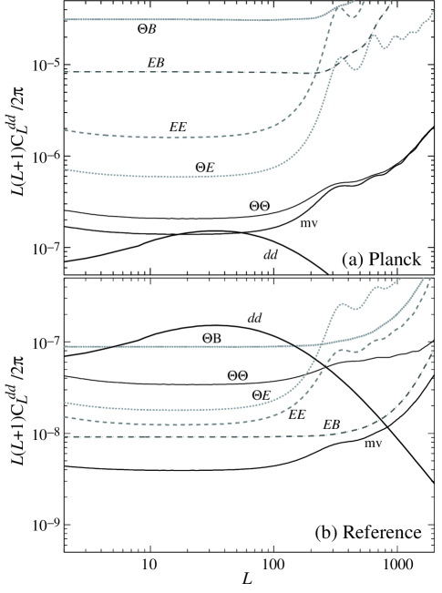
Figure 3.— Deflection signal ($dd$) and noise power spectra of the quadratic estimators and their minimum variance (mv) combination: (a) Planck experiment (b) reference experiment. As the sensitivity of the experiment improves the best quadratic estimator switches from $\Theta\Theta$ to $EB$. Only the $EB$-estimator can reconstruct the mass distribution at $L\gtrsim 200$.

The noise properties of these estimators follows from

$$\langle d_{\alpha}^{*}({{\bf L}})d_{\beta}({{\bf L}}^{\prime})\rangle = (2\pi)^{2}\delta({{\bf L}}-{{\bf L}^{\prime}})[C_{L}^{dd}+N_{\alpha\beta}(L)]\,,$$ (15)

where

$$N_{\alpha\beta}(L) = L^{-2}A_{\alpha}(L)A_{\beta}(L)\int{d^{2}l_{1}\over(2\pi)^{2}}F_{\alpha}({\bf l}_{1},{\bf l}_{2})\Big{(}F_{\beta}({\bf l}_{1},{\bf l}_{2})$$ (16)

$$\times C_{l_{1}}^{x_{\alpha}x_{\beta}}C_{l_{2}}^{x_{\alpha}^{\prime}x_{\beta}^{\prime}}+F_{\beta}({\bf l}_{2},{\bf l}_{1})C_{l_{1}}^{x_{\alpha}x_{\beta}^{\prime}}C_{l_{2}}^{x_{\alpha}^{\prime}x_{\beta}}\Big{)}\,.$$

Recall that the $xx$-power spectra account for both the cosmic variance of the fields and the noise variance of the experiment. Notice that for the minimum variance filter

$$N_{\alpha\alpha}(L)=A_{\alpha}(L)\,.$$ (17)

In Fig. 3, we compare the signal and noise power spectra for the Planck experiment and the reference experiment defined in §2. Recall that true mapping is possible when the signal exceeds the noise spectrum. For the Planck experiment, $\Theta\Theta$ provides the best estimator reflecting the fact that Planck will not be able to produce true maps of the polarization modes. Furthermore, the signal-to-noise is highest at $L\lesssim 200$ reflecting the fact the modes are mainly correlated across $\Delta L\sim 60$, where the deflection power spectrum peaks.

For the reference experiment, all 5 estimators have sufficient signal-to-noise to produce maps at $L\lesssim 200$. The $EB$ estimator has the best signal-to-noise, and allows for mapping to $L\lesssim 1000$. The reason is that there is no noise variance contributed by an unlensed $B$ field. Furthermore, the signal intrinsically comes from higher $L$. A $B$-field at a wavenumber ${\bf l}$ cannot be generated from neighboring modes ${\bf l}^{\prime}\sim{\bf l}$ from the low $L$ deflection field because of the $\sin$ term in the lensing kernel (see Eqn. 2). Thus the signal to noise is relatively higher at high $L$ in the $EB$ estimator.

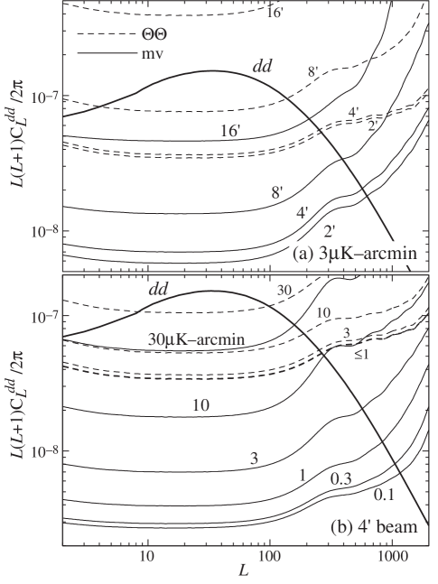
Figure 4.— Deflection signal ($dd$) and noise power spectra for the minimum variance (mv; solid lines) and $\Theta\Theta$ (dashed lines) estimators as a function of (a) beam size $\sigma$ and (b) noise level $\Delta_{T}=\Delta_{P}/\sqrt{2}$. The noise saturates to its minimum by $\sigma\approx 2-4^{\prime}$ and $\Delta_{T}\approx 0.1-0.3\mu$K-arcmin as the polarization field is mapped to the cosmic variance limit out to $l<2000$.

   

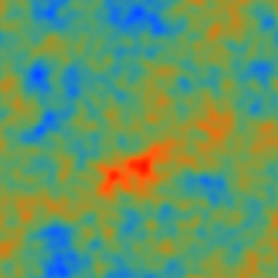
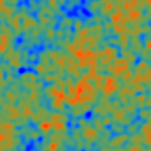
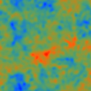
Figure 5.— Mass reconstruction on a $10^{\circ}\times 10^{\circ}$ field with the reference experiment ($\Delta_{T}=\Delta_{P}/\sqrt{2}=1\mu$K-arcmin and $\sigma=4^{\prime}$): (a) deflection field, (b) $\Theta\Theta$-reconstruction, (c) $EB$-reconstruction.

For experiments that are intermediate in sensitivity between Planck and the reference experiment, the five estimators of the deflection field have comparable signal-to-noise and may be used to cross check each other. At high-$L$ where the individual estimators are noise limited, combining the estimators as

$$d_{\rm mv}({{\bf L}})=\sum_{\alpha}w_{\alpha}(L)d_{\alpha}({{\bf L}})\,,$$ (18)

can substantially reduce the noise. The minimum variance weighting is a generalization of the inverse variance weighting that accounts for the covariance in Eqn. (16)

$$w_{\alpha}={\sum_{\beta}({\bf N}^{-1})_{\alpha\beta}\over\sum_{\beta\gamma}({\bf N}^{-1})_{\beta\gamma}}\,.$$ (19)

The noise variance

$$\langle d_{\rm mv}^{*}({\bf L})d_{\rm mv}({\bf L}^{\prime})\rangle=(2\pi)^{2}\delta({\bf L}-{\bf L}^{\prime})[C_{L}^{dd}+N_{\rm mv}(L)]$$ (20)

becomes

$$N_{\rm mv}={1\over\sum_{\alpha\beta}({\bf N}^{-1})_{\alpha\beta}}\,.$$ (21)

Note that the $\Theta\Theta$ and $EB$ estimators are independent and those estimators that are correlated have correlation coefficients $N_{\alpha\beta}/\sqrt{N_{\alpha\alpha}N_{\beta\beta}}$ of no more than tens of percents.

The minimum variance noise spectra for Planck and the reference experiment are shown in Fig. 3. We give it as a function of the noise $\Delta_{T}$ and beam $\sigma$ in Fig. 4. The signal-to-noise saturates around $\Delta_{T}\approx 0.1-0.3\mu$K-arcmin and $\sigma\approx 2-4^{\prime}$. Below $\Delta_{T}\approx 26\mu$K-arcmin ($\Delta_{P}\approx 37\mu$K-arcmin), the combined signal-to-noise in the $\Theta E$ and $EE$ estimators exceeds that in $\Theta\Theta$ at $L\approx 40$ and $\sigma=4^{\prime}$. For the smaller scales of $L\approx 300$, where only the $EB$ estimator plays a role, the $EB$ and $\Theta\Theta$ estimators have comparable signal-to-noise around $\Delta_{T}\approx 6\mu$K-arcmin ($\Delta_{P}\approx 8\mu$K-arcmin) at $L\approx 300$ and $\sigma=4^{\prime}$.

4. EB Estimator

As we have seen in the previous section, the $EB$-estimator of the deflection field has the potential to map the mass distribution out to $L\approx 1000$. We therefore explicitly construct and test this estimator in this section. This construction is very similar to that of the $\Theta\Theta$ estimator presented in Hu (2001b).

From Eqn. (9), the $EB$ estimator is

$$d_{EB}({{\bf L}})={A_{EB}(L)\over L}\int{d^{2}l\over(2\pi)^{2}}E({\bf l})B({\bf l}^{\prime}){\tilde{C}_{l}^{EE}{{\bf L}}\cdot{\bf l}\over C_{l}^{EE}C_{l^{\prime}}^{BB}}\sin 2\varphi_{{\bf l}{\bf l}^{\prime}}\,,$$ (22)

where recall ${\bf L}={\bf l}+{\bf l}^{\prime}$. The convoluted form of this estimator suggests that it may be re-expressed as a product of fields on the sky. To see this, rewrite

$$\sin 2\varphi_{{\bf l}{\bf l}^{\prime}}=2({\hat{\bf l}\cdot\hat{\bf l}^{\prime}})[\hat{\bf n}\cdot({\hat{\bf l}\times\hat{\bf l}^{\prime}})]\,,$$ (23)

where $\hat{\bf n}=-{\bf e}_{3}$. We can then define the filtered fields

$$E_{ijk}(\hat{\bf n}) = \int{d^{2}l\over(2\pi)^{2}}l(\hat{l}_{i}\hat{l}_{j}\hat{l}_{k}){\tilde{C}_{l}^{EE}\over C_{l}^{EE}}E({\bf l})e^{i{\bf l}\cdot\hat{\bf n}}\,,$$ (24)

$$B_{ij}(\hat{\bf n}) = \int{d^{2}l\over(2\pi)^{2}}(\hat{l}_{i}\hat{l}_{j}){1\over C_{l}^{BB}}B({\bf l})e^{i{\bf l}\cdot\hat{\bf n}}\,.$$ (25)

There are $4$ unique filtered $E$-fields and $3$ unique filtered $B$-fields. They may be combined to form the appropriate dot and cross products

$$G_{i}(\hat{\bf n})=2\sum_{jkm}E_{ijk}(\hat{\bf n})B_{jm}(\hat{\bf n})\epsilon_{km3}\,,$$ (26)

where $\epsilon_{ijk}$ is the Levi-Civita symbol. The deflection field is then reconstructed as

$$d_{EB}({\bf L})=-{A_{EB}(L)\over L}{{\bf L}}\cdot{\bf G}({{\bf L}})\,.$$ (27)

The other quadratic estimators can be constructed in a similar fashion.

Fig. 5 shows an example of the $EB$ reconstruction compared with the $\Theta\Theta$ reconstruction on a $10^{\circ}\times 10^{\circ}$ field with the reference experiment. Notice that the $EB$-reconstruction has substantially lower noise on small angular scales. We assume here that the unlensed power spectra have been determined externally from precision satellite missions and through the modelling with cosmological parameters (see Hu 2001b). Errors in the determination translate into non-optimal filters and a small bias in the amplitude of the reconstructed maps.

5. Applications

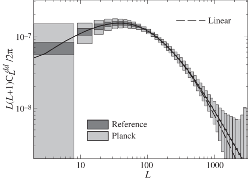
Figure 6.— Statistical errors achievable on the deflection power spectrum with the Planck ($f_{\rm sky}=0.65$) and reference experiments ($f_{\rm sky}=1$). Boxes represent band averaging width and 1$\sigma$ errors. The polarization information in the reference experiment allows for a cosmic variance limited measurement of the projected power spectrum out to $L\sim 1000$. In this regime, the fluctuations are almost completely linear (dashed lines).

In this section, we outline four applications for mass reconstruction: measurement of the (linear) power spectrum in projection, cross correlation with cosmic shear observations, cross correlation with the temperature field, and decontamination of the polarization signature of gravitational waves. The first three applications have been extensively discussed in Hu (2001c) for the $\Theta\Theta$ temperature based estimator and we refer the reader to details therein. Here we focus on the additional information provided by the polarization field.

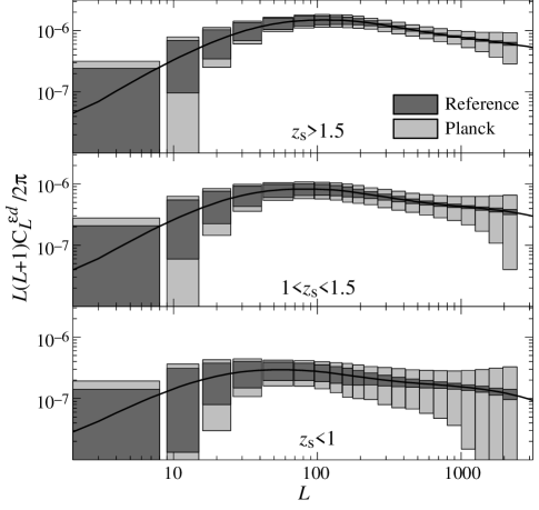
Figure 7.— Statistical errors on the cross correlation of CMB deflections and cosmic shear in three source redshift bands on a $1000$ deg² patch of sky for the Planck and reference experiment. Assumptions for the cosmic shear experiment are given in the text. Precision measurements from the polarization estimators enables highly significant cross correlation detection and hence tomographic studies of structure evolution.

5.1. Linear Power Spectrum

The most direct application of mass reconstruction is to measure the matter power spectrum in projection, i.e. the deflection power spectrum $C_{L}^{dd}$ itself. Power spectrum measurement requires only a statistical detection of the deflection field, not a true reconstructed map and therefore can be extended to higher wavenumbers or smaller scales than is possible for mapping. The noise level for the estimation of band powers is reduced by averaging over ${\bf L}$ directions in a band $\Delta L$

$$\Delta C_{L}^{dd}\approx{1\over\sqrt{L\Delta Lf_{\rm sky}}}[C_{L}^{dd}+N_{\rm mv}(L)]\,,$$ (28)

where $f_{\rm sky}$ is the fraction of the sky covered by the experiment. In this approximation, the noise is assumed to be Gaussian. This should be a good approximation where the sample variance of the lenses dominates the noise variance. Formally, the noise will be increasingly non-Gaussian at high $L$ as the estimator is constructed out of fewer arcminute scale temperature and polarization fluctuations. Quantification of this effect for the temperature based reconstruction show that its effects are minor (Hu 2001a); a full treatment requires the consideration of the temperature-polarization trispectrum (Okamoto & Hu, in prep.).

Polarization enables two advances over what can be achieved by the temperature field alone. As in the case of mapping, polarization enables precision measurements at small scales through the $EB$-estimator. In Fig. 6, we compare the Planck experiment (with $f_{\rm sky}=0.65$) and the reference experiment (with $f_{\rm sky}=1$); as seen in Fig. 3, former relies mainly on the $\Theta\Theta$-estimator and the later on the $EB$-estimator. The noise in the Gaussian approximation approaches the sample variance limit of $\Delta C_{L}^{dd}/C_{L}^{dd}=(L\Delta Lf_{\rm sky})^{-1/2}$ on the scales $L\lesssim 1000$, i.e. a total of 1% precision in each 1% of sky. This corresponds to scales in the matter power spectrum of $0.002\lesssim k\lesssim 0.2$ in $h$/Mpc representing the whole linear regime today.

Equally importantly, the polarization allows for sharp consistency tests on the power spectrum measurements at $L\lesssim 500$. In the reference experiment, all 5 estimators have sufficient signal-to-noise to measure the power spectrum here. It is highly unlikely that any unknown contaminant from foregrounds or instrumental systematics would affect specific quadratic combinations of the temperature, $E$-polarization, $B$-polarization, in the same way.

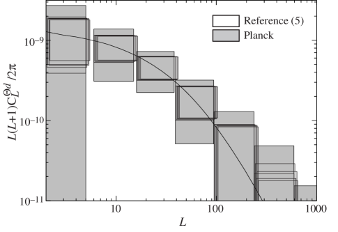
Figure 8.— Statistical errors on the cross correlation of CMB deflections and the temperature field for the Planck ($f_{\rm sky}=0.65$) and reference ($f_{\rm sky}=1$) experiments. The five estimators of the deflection field obtainable with polarization information enables five nearly independent, cosmic variance limited detections of the cross correlation for $L<100$ (shown offset slightly for clarity). The cross correlation is extremely sensitive to the properties of the dark energy.

5.2. Evolution of Structure and Cosmic Shear

One would like to go beyond the projected power spectrum to the three-dimensional distribution to track the evolution of structure and hence the physical properties of the dark matter and energy. This is not possible through CMB lensing alone since the source plane lies at the effectively infinite redshift of last-scattering. Weak lensing also distorts the shape of distant, but for our purposes foreground, galaxies allowing a measurement of the gradient of the deflection angles, or more properly, the so-called cosmic shear, from wide-field imaging surveys (see Mellier 1999; Bartelmann & Schneider 2001 for reviews). Since these sources are distributed across a range of redshifts, the change in the mass reconstruction as a function of source redshift can probe the radial distribution of matter tomographically (Wittman et al. 2001). The effect on the power spectra and cross-correlation of cosmic shear $C_{L}^{\epsilon\epsilon}$ has been shown to be an effective probe of the dark energy equation of state (Huterer 2001; Hu 2001c). Because cosmic shear studies are most effective for $L\gtrsim 100$, tomography with the lensing of the CMB temperature is difficult.

By extending the measurements to overlapping wavenumbers, CMB polarization allows tomographic studies to be anchored at the high-$z$ end. In Fig. 7, we show the errors on the CMB deflection-cosmic shear cross power spectrum $C_{L}^{\epsilon d}$ achievable with the Planck vs. reference experiment and $1000$ deg² of overlap with a cosmic shear survey out to median source redshift $z=1$, divided into three redshift bands $z_{s}<1$, $1<z_{s}<1.5$, $z_{s}>1.5$. Errors on the cosmic shear side assume $n=56$ gal/arcmin², and an intrinsic shear measurement error of $\langle\gamma_{\rm int}\rangle^{2}=0.4$ per component per galaxy.

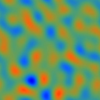
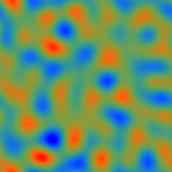
Figure 9.— Large-angle ($l<100$) lensing $B$-polarization field (top) and the reconstructed $B$-polarization field from the small angle $EB$ deflection estimator and the observed $E$-field. Detector noise appropriate for the reference experiment has been added to this $25^{\circ}\times 25^{\circ}$ patch. Reconstruction techniques can help separate the gravitational wave and lensing $B$-modes.

5.3. Dark Energy and the ISW Effect

The integrated Sachs-Wolfe (ISW) effect from the differential redshift due to the decay in the gravitational potential is extremely sensitive to the background properties of the dark energy (Coble et al. 1997; Caldwell et al. 1998) and provides a unique handle on its clustering properties (Hu 1998). The latter can potentially test the scalar-field hypothesis for its nature. Unfortunately the ISW effect is buried under the larger primary anisotropy and can best be isolated through cross correlation with other large-scale tracers of the gravitational potential. The deflection field of CMB lensing provides a perfect candidate for cross correlation (Seljak & Zaldarriaga 1998, Goldberg & Spergel 1999, Hu 2001c). In a flat universe, detection of any cross-correlation at all represents an essentially direct detection of the dark energy.

Since the cross correlation effect is confined to multipoles $L\lesssim 100$, the $\Theta\Theta$ estimator can itself reach the cosmic variance limit for detection. What polarization provides is 4 other nearly independent probes of the cross-correlation. Furthermore the polarization estimators each contain enough signal-to-noise to reconstruct the deflection field with independent sets of multipoles in the polarization field (see Hu 2001 for the analogous technique using the temperature field). Since the signal is weak and the importance of understanding the particle properties of the dark energy great, the ability to make these consistency tests is an important asset.

In Fig. 8, we compare the ability of the Planck experiment $(f_{\rm sky}=0.65)$ and the reference experiment $(f_{\rm sky}=1)$ to measure the deflection-ISW cross correlation $C_{L}^{\Theta d}$.

5.4. Gravitational Waves and $B$-modes

The $B$-mode polarization produced by gravitational waves offers what is perhaps our most direct window on the early universe (Kamionkowski, Kosowsky & Stebbins 1997; Zaldarriaga & Seljak 1997). Under the inflationary paradigm, its amplitude determines the energy scale of inflation. In this context, gravitational lensing, which also generates $B$-modes acts as a contaminant. To constrain inflationary energy scales below $10^{16}$ GeV, removal of the lensing contaminant, either statistical or direct, will be required (Hu 2001c). Fortunately the converse problem does apply: since the $B$-modes used to reconstruct the deflection fields reside in the arcminute regime, even much larger amplitude gravitational wave $B$-modes at degree scales do not contaminate mass reconstruction. This fact allows the possibility of direct removal of the lensing $B$-modes at degree scales.

We save detailed exploration of $B$-mode decontamination to a future work and here simply show that the mass reconstruction from the small-scale $B$-polarization itself has sufficient signal-to-noise to make the procedure feasible. Decontamination is not feasible through the $\Theta\Theta$ estimator since most of the $B$-modes on degree scales arise from fluctuations in the deflection field with $L\gtrsim 200$.

Consider the $E$-modes of the observed, i.e. lensed and including detector noise, polarization field and construct the Stokes parameters $Q(\hat{\bf n})$ and $U(\hat{\bf n})$ from it alone via Eqn. (2). Use the reconstructed deflection field $d_{EB}(\hat{\bf n})$ to artificially lens the distribution. The $B$-field of the resulting polarization is an estimator of the $B$-field from lensing that is independent of the true $B$-field on large scales. In Fig. 9, we show the true $B$-field from lensing, low pass filtered to $l<100$, compared with the reconstructed $B$-field for the reference experiment on a $25^{\circ}\times 25^{\circ}$ field.

6. Discussion

Based on the induced correlation between the $E$ and $B$ modes, the lensing of CMB polarization offers the opportunity to reconstruct the mass distribution in projection on scales corresponding to $0.002<k<0.2$ in $h$ Mpc^-1. Compared with a similar reconstruction from the temperature field, polarization allows for an order of magnitude extension to smaller scales. These small scales can correspondingly be probed with the smaller degree scale fields of view that are more typical for planned polarization studies. Moreover mass reconstruction is only sensitive to the arcminute scale correlations in the polarization field and does not require a true map over the full field. This additional range does not come at the expense of higher resolution requirements: the signal-to-noise saturates at the several arcminute scale corresponding to $l\approx 2000$. Due to the smaller absolute scale of the signal, polarization studies do require much more sensitive detectors, with the $EB$ estimator surpassing the $\Theta\Theta$ estimator for $\Delta_{P}\lesssim 8\mu$K-arcmin for $L\sim 300$. Sensitivity and control over foregrounds and systematics are issues that any polarization based study must address, especially those searching for the gravitational wave imprint from inflation.

Mass reconstruction from CMB polarization can provide measurements of the matter power spectrum over a wide range of scales that are entirely free of assumptions of how the luminous matter traces the mass (or bias) and the distribution of lensing sources, as well as largely free of non-linear corrections. It complements cosmic shear studies by providing the deepest two-dimensional mass maps possible to anchor tomographic studies of the evolution of structure. It extends the shear-based lensing studies to near horizon-sized structures and therefore provides the opportunity to study the dark energy in its cross correlation with the ISW effect in the temperature field. Finally, since reconstruction only requires information from fine-scale correlations in the polarization field, it may be used to remove the lensing $B$-modes on large-scales from any potential gravitational wave signal. These potential scientific returns may help justify the great experimental effort that will be required to map the CMB polarization field.

Acknowledgments: We thank Bruce Winstein and Matias Zaldarriaga for useful discussions. This work was supported by NASA NAG5-10840 and the DOE OJI program.

References

- (1)
- (2) Bartelmann, M. Schneider, P. 2001, Phys. Rept., 340, 291.
- (3) Benabed, K. Bernardeau, F. van Waerbeke, L. 2001, Phys. Rev. D, 63, 043501.
- (4) Bernardeau, F. 1997, A&A, 324, 15.
- (5) Blanchard, A. Schneider, J. 1987, A&A, 184, 1.
- (6) Caldwell, R.R. Dave, R. Steinhardt, P.J. 1998, Phys. Rev. Lett., 80, 1582.
- (7) Coble, K. Dodelson, S. Frieman, J.A. 1997, Phys. Rev. D, 55, 1851.
- (8) Cooray, A.R. Hu, W. 2000, ApJ, 534, 533.
- (9) Goldberg, D.M. Spergel, D.N. 1999, Phys. Rev. D, 59, 103002.
- (10) Guzik, J. Seljak, U. Zaldarriaga, M. 2000, Phys. Rev. D, 62, 043517.
- (11) Hu, W. 1998, ApJ, 506, 485.
- (12) Hu, W. 2000a, ApJ, 529, 12.
- (13) Hu, W. 2000b, Phys. Rev. D, 62, 043007.
- (14) Hu, W. 2001a, Phys. Rev. D, in press, astro-ph/0105117.
- (15) Hu, W. 2001b, ApJ Lett., 557, L79.
- (16) Hu, W. 2001c, Phys. Rev. D, in press, .
- (17) Huterer, D. 2001, Phys. Rev. D, in press, .
- (18) Kaiser, N. Squires, G. 1993, ApJ, 404, 441.
- (19) Kamionkowski, M. Kosowsky, A. Stebbins, A. 1997, Phys. Rev. D, 55, 7368.
- (20) Knox, L. 1995, Phys. Rev. D, 52, 4307.
- (21) Mellier, Y. 1999, ARA&A, 37, 127.
- (22) Seljak, U. 1996, ApJ, 463, 1.
- (23) Seljak, U. Zaldarriaga, M. 1999, Phys. Rev. D, 60, 043504.
- (24) Wittman, D. Tyson, J.A. Margoniner, V.E. Cohen, J.G. Dell’Antonio, I.P. 2001, ApJ, 557, 89.
- (25) Zaldarriaga, M. 2000, Phys. Rev. D, 62, 063510.
- (26) Zaldarriaga, M. Seljak, U. 1997, Phys. Rev. D, 55, 1830.
- (27) Zaldarriaga, M. Seljak, U. 1998, Phys. Rev. D, 58, 023003.
- (28) Zaldarriaga, M. Seljak, U. 1999, Phys. Rev. D, 59, 123507.