¹NORDITA, Blegdamsvej 17, DK-2100 Copenhagen Ø, Denmark
²Department of Mathematics, University of Newcastle, NE1 7RU, UK
³Kiepenheuer-Institut für Sonnenphysik, Schöneckstr. 6, 79104 Freiburg, Germany

Hydromagnetic turbulence in computer simulations

1 Introduction

Hydromagnetic processes play an important role in many astrophysical systems (e.g. stars, galaxies, accretion discs). This is because the medium is hot enough to be partially or fully ionized. Because of the huge scales involved the medium is usually turbulent, provided there is an instability (shear, convection) facilitating the cascading of energy down to small scales.

In turbulence research it has been a long standing tradition to solve the hydrodynamic equations using spectral schemes which have the lowest possible discretization error. Spectral schemes are particularly useful for incompressible problems where one needs to solve a Poisson-type equation for the pressure. However, spectral schemes are no longer optimal in many astrophysical circumstances where flows are generally compressible. Lower order spatial derivative schemes are generally unacceptable in view of their low overall accuracy, even when schemes are used where mass, momentum, and energy are conserved to machine accuracy. On massively parallel machines, on the other hand, spectral schemes are difficult to make run efficiently. High order finite difference schemes are therefore a useful compromise. Such schemes can yield almost spectral-like accuracy.

Our code uses centered finite differences which make the adaptation to other problems simple. Since the code is not written in conservative form, conservation of mass, energy and momentum can be used to monitor the quality of the solution. A third order Runge-Kutta scheme with $2N$ storage [1] is used for calculating the time advance.

2 Advantages of high-order schemes

Spectral methods are commonly used in almost all studies of ordinary (usually incompressible) turbulence. The use of this method is justified mainly by the high numerical accuracy of spectral schemes. Alternatively, one may use high-order finite differences that are faster to compute and that can possess almost spectral accuracy. In astrophysics, high-order compact finite differences [2] have been used to model stellar convection [3, 4] and shear flows in accretion discs [5]. In contrast to explicit finite differences, compact finite differences [2] have a smaller coefficient in the leading error, even if both schemes are of the same order. However, compact schemes are still nonlocal in the sense that each point affects every other point, which enhances communication. This is the main reason why we adopt explicit centered finite differences.

In this section we demonstrate, using simple test problems, some of the advantages of high-order schemes. The explicit formulae for first and second derivatives are

$$f^{\prime}_{i}=(-f_{i-3}+9f_{i-2}-45f_{i-1}$$

$$+45f_{i+1}-9f_{i+2}+f_{i+3})/(60\delta x),$$ (1)

$$f^{\prime\prime}_{i}=(2f_{i-3}-27f_{i-2}+270f_{i-1}-490f_{i}$$

$$+270f_{i+1}-27f_{i+2}+2f_{i+3})/(180\delta x^{2}).$$ (2)

Full details of these schemes, including formulae for the boundaries, can be found in Ref. [6]. This scheme was also used in recent applications to the problem of resistively limited growth in models of stellar dynamos; see Ref. [7].

It is commonly believed that high-order schemes lead to Gibbs phenomena and that more viscosity is needed to damp them out. In fact, the opposite is true as is demonstrated in Fig. 1 for advection tests and in Fig. 2 for the stationary Burgers shock.

Figure 1: Advection tests with schemes of different spatial order. Resulting profile after advecting a step-like function 5 times through the periodic mesh. The dots on the solid line give the location of the function values at the computed meshpoints and the dotted line gives the original profile. For the panels on the right hand side the diffusion coefficient is too small and the profile shows noticeable wiggles. $\delta x=1/60$.

Figure 2: Burgers shock with schemes of different spatial order and different values of the viscosity. The solid lines give the analytic solution. A second order scheme (top row) requires a viscosity of at least $0.8u\delta x$, where $u$ is the amplitude of the shock and $\delta x$ the mesh spacing. For a sixth-order scheme, a viscosity of $0.6u\delta x$ yields good results, and for a tenth-order scheme a viscosity of $0.5u\delta x$ can be used.

For the time stepping high-order schemes are necessary in order to reduce the amplitude error of the scheme and to allow longer time steps. Usually such schemes require large amounts of memory. However, there are the memory-effective $2N$-schemes that require only two sets of variables to be held in memory. Such schemes work for arbitrarily high order, although not all Runge-Kutta schemes can be written as $2N$-schemes [1, 8]. These schemes work iteratively according to the formula

$$w_{i}=\alpha_{i}w_{i-1}+\delta t\,F(t_{i-1},u_{i-1}),$$ (3)

$$u_{i}=u_{i-1}+\beta_{i}w_{i}.$$ (4)

For a three-step scheme we have $i=1,...,3$. In order to advance the variable $u$ from $u^{(n)}$ at time $t^{(n)}$ to $u^{(n+1)}$ at time $t^{(n+1)}=t^{(n)}+\delta h$ we set in Eq. (4)

$$u_{0}=u^{(n)}\quad\mbox{and}\quad u^{(n+1)}=u_{3},$$ (5)

with $u_{1}$ and $u_{2}$ being intermediate steps. In order to be able to calculate the first step, $i=1$, for which no $w_{i-1}\equiv w_{0}$ exists, we have to require $\alpha_{1}=0$. Thus, we are left with 5 unknowns, $\alpha_{2}$, $\alpha_{3}$, $\beta_{1}$, $\beta_{2}$, and $\beta_{3}$. Three conditions follow from the fact that the scheme be third order, so we have to have two more conditions. One possibility is the choose the fractional times at which the right hand side is evaluated, for example (0, 1/3, 2/3) or even (0, 1/2, 1). In the latter case the right hand side is evaluated twice at the same time. It is therefore some sort of predictor-corrector scheme. Yet another possibility is to require that inhomogeneous equations of the form $\dot{u}=t^{n}$ with $n=1$ and 2 are solved exactly. The corresponding coefficients are listed in Table LABEL:Ttab_2N-RK3 and compared with those given by Williamson [1]. In practice all of them are about equally good when it comes to real applications, although we found the first one in Table LABEL:Ttab_2N-RK3 (‘symmetric’) marginally better in some simple test problems where an analytic solution was known.

Table 1: Possible coefficients for different $2N$-RK3 schemes.

label $\alpha_{2}$ $\alpha_{3}$ $\beta_{1}$ $\beta_{2}$ $\beta_{3}$ symmetric $-2/3$ $-1$ 1/3 1 1/2 predictor/corrector $-1/4$ $-4/3$ 1/2 2/3 1/2 inhomogeneous $-17/32$ $-32/27$ 1/4 8/9 3/4 Williamson (1980) $-5/9$ $-153/128$ 1/3 15/16 8/15

3 Implementing magnetic fields

Implementing magnetic fields is relatively straightforward. On the one hand, the magnetic field causes a Lorentz force, ${\bf{J}}\times{\bf{B}}$, where ${\bf{B}}$ is the flux density, ${\bf{J}}=\mbox{\boldmath$\nabla$}{}\times{\bf{B}}/\mu_{0}$ is the current density, and $\mu_{0}$ is the vacuum permeability. On the other hand, ${\bf{B}}$ itself evolves according to the Faraday equation,

$${\partial{\bf{B}}\over\partial t}=-\mbox{\boldmath$\nabla$}{}\times{\bf{E}}$$ (6)

where the electric field ${\bf{E}}$ can be expressed in terms of ${\bf{J}}$ using Ohm’s law in the laboratory frame, ${\bf{E}}=-{\bf{u}}\times{\bf{B}}+{\bf{J}}/\sigma$, where $\sigma=(\eta\mu_{0})^{-1}$ is the electric conductivity and $\eta$ is the magnetic diffusivity.

In addition we have to satisfy the condition $\mbox{\boldmath$\nabla$}{}\cdot{\bf{B}}=0$. This is most easily done by solving not for ${\bf{B}}$, but instead for the magnetic vector potential ${\bf{A}}$, where ${\bf{B}}=\mbox{\boldmath$\nabla$}{}\times{\bf{A}}$. The evolution of ${\bf{A}}$ is governed by the uncurled form of Eq. (6),

$${\partial{\bf{A}}\over\partial t}=-{\bf{E}}-\mbox{\boldmath$\nabla$}{}\phi$$ (7)

where $\phi$ is the electrostatic potential, which takes the role of an integration constant which does not affect the evolution of ${\bf{B}}$. The choice $\phi=0$ is most advantageous on numerical grounds. (By contrast, the Coulomb gauge $\nabla\cdot{\bf{A}}=0$, which is very popular in analytic considerations, would obviously be of no advantages, since one still has the problem of solving a the solenoidality condition.

Solving for ${\bf{A}}$ instead of ${\bf{B}}$ has significant advantages, even though this involves taking another derivative. However, the total number of derivatives taken in the code is essentially the same. In fact, when centered finite differences are employed, Alfvén waves are better resolved when ${\bf{A}}$ is used, because then the system of equations for one-dimensional Alfvén waves in the presence of a uniform $B_{x0}$ field in a medium of constant density $\rho_{0}$ reduces to

$$\dot{u}_{z}=(\mu_{0}\rho_{0})^{-1}B_{x0}A_{y}^{\prime\prime},\quad\dot{A}_{y}=B_{x0}u_{z},$$ (8)

where a second derivative is taken only once (primes denote $x$-derivatives). If, instead, one solves for the $B_{z}$ field, one has

$$\dot{u}_{z}=(\mu_{0}\rho_{0})^{-1}B_{x0}B_{z}^{\prime},\quad\dot{B}_{z}=B_{x0}u_{z}^{\prime},$$ (9)

where a first derivative is applied twice, which is far less accurate at small scales if a centered finite difference scheme is used. At the Nyquist frequency, for example, the first derivative is zero and applying an additional first derivative gives still zero. By contrast, taking a second derivative once gives of course not zero. The use of a staggered mesh would circumvent this difficulty. However, such an approach introduces additional complications which hamper the ease with which the code can be adapted to new problems.

Another advantage of using ${\bf{A}}$ is that it is straightforward to evaluate the magnetic helicity, $\langle{\bf{A}}\cdot{\bf{B}}\rangle$, which is a particularly important quantity to monitor in connection with dynamo and reconnection problems.

The main advantage of solving for ${\bf{A}}$ is of course that one does not need to worry about the solenoidality of the ${\bf{B}}$-field, even though one may want to employ irregular meshes or complicated boundary conditions.

4 Cache-efficient coding

Unlike the CRAY computers that dominated supercomputing in the 80ties and early 90ties, all modern computers have a cache that constitutes a significant bottleneck for many codes. This is the case if large three-dimensional arrays are constantly used within each time step. The advantage of this way of coding is clearly the conceptual simplicity of the code. A more cache-efficient way of coding is to calculate an entire timestep (or a corresponding substep in a three-stage $2N$ Runge-Kutta scheme) only along a one-dimensional pencil of data within the box. On Linux and Irix architectures, for example, this leads to a speed-up by 60%. An additional advantage is a drastic reduction in temporary storage that is needed for auxiliary variables within each time step.

5 Large scale fields from helical turbulence

Many astrophysical flows are affected by rotation and gravitational stratification. These two effects can make the flows helical. In the sun, for example, the kinetic helicity of the flow is negative in the northern hemisphere and positive in the southern. It has long been known that this can lead to the production of large scale magnetic fields [9].

Recent simulations of helically forced turbulence have shown that large scale fields are indeed produced [10]. These large scale fields are approximately force-free and of Beltrami type; see Fig. 3. The prototype of a Beltrami field is $\overline{\bf{B}}\propto(\cos z,\sin z,0)$, and it is easy to see that for this field $\overline{\bf{J}}\times\overline{\bf{B}}=0$, where $\overline{\bf{J}}=\mbox{\boldmath$\nabla$}{}\times\overline{\bf{B}}/\mu_{0}$ is the current density.

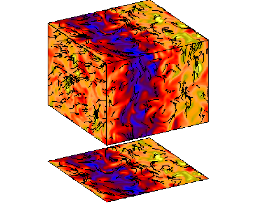
Figure 3: Visualization of the magnetic field in a three-dimensional simulation of helically forced turbulence. The turbulent magnetic field is modulated by a slowly varying component that is force free.

At large scales, force-free Beltrami fields are only possible in a periodic box, as considered in Ref. [10]. When the box in non-periodic, the large scale field can still be ‘nearly periodic’. In simulations with so-called ‘pseudo-vacuum’ boundary conditions, for example, a large scale field of the form

$$\overline{\bf{B}}=(\cos{\textstyle{1\over 2}}z,\sin{\textstyle{1\over 2}}z,0)\cos{\textstyle{1\over 2}}z$$ (10)

appeared; see Ref. [7]. We now consider the case of perfectly conducting boundaries. Unlike the case of pseudo-vacuum boundary conditions, where the energy of the large scale field was somewhat below the kinetic energy, with perfectly conducting boundaries the energy of the large scale field can strongly exceed the kinetic energy of the turbulence; see Fig. 4.

Figure 4: Evolution of magnetic and kinetic energies, $E_{\rm M}$ and $E_{\rm K}$, respectively, in a simulation with perfectly conducting boundaries.

The resulting super-equipartition of large scale magnetic energy is primarily a consequence of the fact that the large scale field is force-free and does not act back on the flow. Force-free fields are generally helical and have to obey the equation of magnetic helicity conservation,

$${\rm d}{}\langle{\bf{A}}\cdot{\bf{B}}\rangle/{\rm d}{}t=-2\eta\mu_{0}\langle{\bf{J}}\cdot{\bf{B}}\rangle.$$ (11)

The precise saturation level is obtained from the fact that in the steady state the magnetic helicity, $\langle{\bf{A}}\cdot{\bf{B}}\rangle$, is constant. This implies that the current helicity, $\langle{\bf{J}}\cdot{\bf{B}}\rangle$, vanishes. Now, splitting the field into large and small scale components, ${\bf{B}}=\overline{\bf{B}}+{\bf{b}}$, we have $\langle\overline{\bf{J}}\cdot\overline{\bf{B}}\rangle=-\langle{\bf{j}}\cdot{\bf{b}}\rangle$. Assuming that the fields are fully helical at small and large scales, we have $\mu_{0}\langle\overline{\bf{J}}\cdot\overline{\bf{B}}\rangle=\mp k_{1}\langle\overline{\bf{B}}^{2}\rangle$ and $\mu_{0}\langle{\bf{j}}\cdot{\bf{b}}\rangle=\pm k_{\rm f}\langle{\bf{b}}^{2}\rangle$, where $k_{1}$ is the smallest wavenumber in the box and $k_{\rm f}$ is the wavenumber of the forcing. (Upper/lower signs apply to positive/negative sign of the helicity of the forcing function.) Due to non-periodic boundary condition, however, the large scale field cannot be completely force-free. Therefore we allow for an efficiency factor $\epsilon_{\rm LS}<1$ for the large scales (LS). Thus, the final balance equation is

$$\epsilon_{\rm LS}k_{1}\langle\overline{\bf{B}}^{2}\rangle=k_{\rm f}\langle{\bf{b}}^{2}\rangle,$$ (12)

i.e. the energy of the large scale field exceeds that of the small scale field by a factor $\epsilon_{\rm LS}^{-1}k_{\rm f}/k_{1}$. This is consistent with Fig. 4. Note, for comparison, that for fully periodic boxes, $\epsilon_{\rm LS}=1$ and therefore the factor of superequipartion is only $k_{\rm f}/k_{1}$.

The reason why the magnetic energy saturates in stages is connected with the occurrence of different patterns of the large scale field: at early times the large scale field is dominated by a pattern with a relatively large wavenumber in one of the two horizontal directions (the boundaries are in the vertical direction). Initially the large scale fields has 8 nodal planes, but then it reduces to 4 and finally to 2 nodal planes.

Finally, it should be emphasized that we have discussed here only the details of the saturation behavior. However, when the field is weak the magnetic field grows always exponentially on a dynamical time scale (usually over many orders of magnitude), and is independent of magnetic helicity conservation.

6 Conclusions

The use of high-order schemes proved to be a useful compromise between the cheap, but less accurate low-order methods and the computationally more expensive spectral schemes. Explicit meshpoint schemes can readily be implemented on massively parallel architectures using High Performance Fortran (HPF) or the Message Passing Interface (MPI). The $2N$-schemes of Williamson [1] are ideal for reducing the amount of storage while still allowing the temporal order of the scheme to be high.

Id: paper.tex,v 1.4 2001/09/17 16:34:26 brandenb Exp

References

- [1] Williamson, J. H., J. Comp. Phys. 35, 48 (1980)
- [2] Lele, S. K., J. Comp. Phys. 103, 16 (1992)
- [3] Nordlund, Å., Stein, R. F., Comput. Phys. Commun. 59, 119 (1990)
- [4] Brandenburg, A., et al., J. Fluid Mech. 306, 325 (1996)
- [5] Brandenburg, A., et al., Astrophys. J., 446, 741 (1995)
- [6] Brandenburg, A., in Advances in non-linear dynamos, ed. A. Ferriz-Mas & M. Núñez Jiménez (2001); http://arXiv.org/abs/astro-ph/0109497
- [7] Brandenburg, A., Dobler, W., Astron. Astrophys. 369, 329 (2001)
- [8] Stanescu, D., Habashi, W. G., J. Comp. Phys. 143, 674 (1988)
- [9] Krause, F., Rädler, K.-H., Mean-Field Magnetohy- drodynamics and Dynamo Theory, Akademie-Verlag, Berlin; also Pergamon Press, Oxford (1980)
- [10] Brandenburg, A., Astrophys. J. 550, 824 (2001)