Abstract

We investigate the possibility of reconstructing the initial spectrum of density fluctuations from the cosmic microwave background (CMB) anisotropy. As a first step toward this program, we consider a spatially flat, CDM dominated universe. In this case, it is shown that, with a good accuracy, the initial spectrum satisfies a first order differential equation with the source determined by the CMB angular correlation function. The equation is found to contain singularities arising from zeros of the acoustic oscillations in the transfer functions. Nevertheless, we find these singularities are not fatal, and the equation can be solved nicely. We test our method by considering simple analytic forms for the transfer functions. We find the initial spectrum is reproduced within 5% accuracy even for a spectrum that has a sharp spike.

PACS: 95.30.-k; 98.80.Es

I Introduction

Determination of the primordial spectrum of the density fluctuations is one of the most important issues in modern cosmology. The cosmic microwave background (CMB) anisotropy provides us with a great deal of information of the primordial fluctuations, and it is considered to be a powerful tool for studying the early universe [1]. This is because the physical processes that determine the CMB anisotropy are described by linear perturbation theory, and they have been well understood [2, 3].

Although the recent anisotropy observations are consistent with a flat universe with a scale-invariant initial power spectrum, this does not exclude the possibilities of other models. In particular, we do not know how much the shape of the initial power spectrum is constrained. In most of previous investigations, when cosmological model parameters are estimated from the observational data by likelihood analysis, the initial spectrum is assumed to have a power-law shape [4]. It is true that a conventional slow-roll inflation model [5], that has now become a ‘standard model’, gives a power-law spectrum which is almost scale-invariant[6]. However, when analyzing the observed CMB anisotropy, it is much more desirable, and probably much healthier, to constrain the initial spectrum solely by observed data without any theoretical prejudices. For example, even within the context of inflationary cosmology, a variety of generation mechanisms for non-scale-invariant perturbations have been proposed [7]. In this connection, recently several authors have discussed extraction of non-power law features from the CMB observations [8], where the initial spectrum is allowed to have a piece-wise power-law shape.

In this paper, we approach this issue in an entirely different way, namely, by formulating an inverse problem as faithful as possible. Such an approach will be eventually needed if we seriously want to constrain the initial power spectrum solely from observations of the CMB anisotropy. An approach to this inversion problem has been discussed recently [9].

As a first step, we consider a simple situation in which the transfer functions that relate the input power spectrum $P(k)$ of the gravitational potential to the output CMB angular correlation function $C(\theta)$ are given analytically. This is certainly a toy model. However, it has almost all the essential features a realistic model would have. In particular, unlike [9], our model takes account of not only the Sachs-Wolfe (SW) effect[10] but also the Doppler effect . The latter, which gives rise to zero points in the transfer functions, is the main cause of the difficulty in this inversion problem.

The advantage of adopting this simple situation is that our method of inversion which we shall develop below may be easily tested at various stages of calculations. Since our primary concern here is to formulate the inversion problem, we fix the cosmological parameters and do not study the dependence of $P(k)$ upon them.

The paper is organized as follows. In Sec. II, we give the basic equations that relate the primordial spectrum $P(k)$ with the angular correlation function $C(\theta)$. In Sec. III, under some reasonable assumptions, we derive a differential equation for $P(k)$ and develop a method to solve it. Then we test our method by applying it to several spectral shapes. We find our method is applicable even in the case of a spectrum with a sharp spike.

II Basic Equations

The angular correlation function of the CMB, $C(\theta)$ is defined as

$$C(\theta)=\langle\Theta(\mathchoice{{\hbox{\boldmath$\displaystyle\gamma$}}}{{\hbox{\boldmath$\textstyle\gamma$}}}{{\hbox{\boldmath$\scriptstyle\gamma$}}}{{\hbox{\boldmath$\scriptscriptstyle\gamma$}}}_{1})\Theta(\mathchoice{{\hbox{\boldmath$\displaystyle\gamma$}}}{{\hbox{\boldmath$\textstyle\gamma$}}}{{\hbox{\boldmath$\scriptstyle\gamma$}}}{{\hbox{\boldmath$\scriptscriptstyle\gamma$}}}_{2})\rangle,\hskip 28.45274pt\cos\theta=\mathchoice{{\hbox{\boldmath$\displaystyle\gamma$}}}{{\hbox{\boldmath$\textstyle\gamma$}}}{{\hbox{\boldmath$\scriptstyle\gamma$}}}{{\hbox{\boldmath$\scriptscriptstyle\gamma$}}}_{1}\cdot\mathchoice{{\hbox{\boldmath$\displaystyle\gamma$}}}{{\hbox{\boldmath$\textstyle\gamma$}}}{{\hbox{\boldmath$\scriptstyle\gamma$}}}{{\hbox{\boldmath$\scriptscriptstyle\gamma$}}}_{2}$$ (1)

where $\Theta(\mathchoice{{\hbox{\boldmath$\displaystyle\gamma$}}}{{\hbox{\boldmath$\textstyle\gamma$}}}{{\hbox{\boldmath$\scriptstyle\gamma$}}}{{\hbox{\boldmath$\scriptscriptstyle\gamma$}}})=(\Delta T/\bar{T})(\mathchoice{{\hbox{\boldmath$\displaystyle\gamma$}}}{{\hbox{\boldmath$\textstyle\gamma$}}}{{\hbox{\boldmath$\scriptstyle\gamma$}}}{{\hbox{\boldmath$\scriptscriptstyle\gamma$}}})$ is the temperature fluctuation in the direction $\textstyle\gamma$ and the average is taken over all angles and all spatial positions. $C(\theta)$ is expanded in the Legendre polynomials and related to the angular power spectrum, $C_{l}$, as

$$C(\theta)=\sum_{l}\frac{2l+1}{4\pi}C_{l}P_{l}(\cos\theta).$$ (2)

$C(\theta)$ or $C_{l}$ are the fundamental observables of the CMB anisotropy. Our purpose is to reconstruct the initial power spectrum from the above observables. We calculate in the Newtonian gauge and follow the notation of [3].

Each Fourier mode of temperature perturbations, $\Theta(\eta,\mathchoice{{\hbox{\boldmath$\displaystyle k$}}}{{\hbox{\boldmath$\textstyle k$}}}{{\hbox{\boldmath$\scriptstyle k$}}}{{\hbox{\boldmath$\scriptscriptstyle k$}}})$, obeys the Boltzmann equation [11],

$$\dot{\Theta}+ik\mu(\Theta+\Psi)=-\dot{\Phi}+\dot{\tau}[\Theta_{0}-\Theta-\frac{1}{10}\Theta_{2}P_{2}(\mu)-i\mu V_{b}],$$ (3)

where the dot denotes a derivative with respect to the conformal time $\eta$, $k$ is the comoving wave number, $\mu=k^{-1}\mathchoice{{\hbox{\boldmath$\displaystyle k$}}}{{\hbox{\boldmath$\textstyle k$}}}{{\hbox{\boldmath$\scriptstyle k$}}}{{\hbox{\boldmath$\scriptscriptstyle k$}}}\cdot\mathchoice{{\hbox{\boldmath$\displaystyle\gamma$}}}{{\hbox{\boldmath$\textstyle\gamma$}}}{{\hbox{\boldmath$\scriptstyle\gamma$}}}{{\hbox{\boldmath$\scriptscriptstyle\gamma$}}}$, $\dot{\tau}$ is the differential Thomson optical depth and $V_{b}$ is the bulk velocity of baryons. $\Psi$ and $\Phi$ are the gauge-invariant Newtonian potential and spatial curvature perturbation, respectively[11]. Here, we decompose $\Theta(\eta,k,\mu)$ into the multipole moments,

$$\Theta(\eta,k,\mu)=\sum_{l}(-i)^{l}\Theta_{l}(\eta,k)P_{l}(\mu),$$ (4)

where $\Theta_{l}(\eta,k)$ is the $l$-th multipole moment of $\Theta(\eta,k,\mu)$. Integrating Eq. (3), we obtain

$$(\Theta+\Psi)(\eta_{0},k,\mu)=\int^{\eta_{0}}_{0}\,\left\{[\Theta_{0}+\Psi-i\mu V_{b}]{\cal V}(\eta)+(\dot{\Psi}-\dot{\Phi})e^{-\tau(\eta)}\right\}e^{ik\mu(\eta-\eta_{0})}d\eta,$$ (5)

where $\eta_{0}$ is the conformal time today and ${\cal V}(\eta)$ is the visibility function given by

$${\cal V}(\eta)=\dot{\tau}(\eta)e^{-\tau(\eta)}\,;\quad\tau(\eta)=\int^{\eta_{0}}_{\eta}\dot{\tau}(\eta^{\prime})d\eta^{\prime}.$$ (6)

We have neglected the quadrupole term on the right hand side of Eq. (3) since its contribution is negligible in the tight coupling approximation. The visibility function has a sharp peak around the last scattering time $\eta_{*}$ so that we assume that recombination occurs instantaneously at $\eta=\eta_{*}$. Then, the multipole moments of each $k$ mode is approximately given by

$$\Theta_{l}(\eta_{0},k) = (\Theta_{0}+\Psi)(\eta_{*},k)(2l+1)j_{l}(kd)+\Theta_{1}(\eta_{*},k)(2l+1)j^{\prime}_{l}(kd)$$ (8)

$$+(2l+1)\int^{\eta_{0}}_{\eta_{*}}d\eta^{\prime}\frac{\partial}{\partial\eta^{\prime}}(\Psi(\eta^{\prime},k)-\Phi(\eta^{\prime},k))j_{l}(k\eta_{0}-k\eta^{\prime}),$$

where $d=\eta_{0}-\eta_{*}$ is a conformal distance from the present epoch to the last scattering surface (LSS). Equation (8) shows that there are four sources for the temperature anisotropy, namely, the intrinsic temperature variation, the Sachs-Wolfe (SW) effect which is caused by the static gravitational potential at the last scattering surface and is dominant on large scales, the Doppler effect due to the fluid bulk velocity, and the integrated Sachs-Wolfe (ISW) effect due to the time variation of the metric perturbation after decoupling. If the recombination occurs when the universe is matter-dominated, $\Psi$ and $\Phi$ remain constant in time after decoupling until a stage at which either the curvature term or the cosmological constant term becomes significant. In particular, in the Einstein-de Sitter universe, they remain constant until today, hence the ISW effect is absent.

Conventionally, $C_{l}$ is expressed as

$$\frac{2l+1}{4\pi}C_{l}=\frac{1}{2\pi^{2}}\int^{\infty}_{0}dk\,k^{2}\frac{|\Theta_{l}(\eta_{0},k)|^{2}}{2l+1}\,.$$ (9)

From Eqs. (8) and (9), we find

$$C_{l}=\frac{2}{\pi}\int^{\infty}_{0}dk\,k^{2}\Bigl{[}(\Theta_{0}+\Psi)(\eta_{*})j_{l}(kd)+\Theta_{1}(\eta_{*})j^{\prime}_{l}(kd)\Bigr{]}^{2}.$$ (10)

The angular correlation function is calculated from Eq. (10). Here, we define $r$ by

$$r=2d\sin\frac{\theta}{2}\,.$$ (11)

This is the spatial distance between two points on the last scattering surface which are observed with the angular separation $\theta$. Since the thickness of the LSS is neglected in Eq. (8), there is a one-to-one correspondence between the observed temperature anisotropy and the perturbation variables on the LSS. Using the relation,

$$\sum^{\infty}_{l=0}(2l+1)P_{l}(\cos\theta)j^{2}_{l}(kd)=\frac{\sin kr}{kr}\,,$$ (12)

the angular correlation function $C(r)$ is given by

$$C(r) = \frac{1}{2\pi^{2}}\int^{\infty}_{0}dk\,k^{2}\Biggl{[}|\Theta_{0}+\Psi|^{2}+(\Theta_{0}+\Psi)\Theta_{1}\frac{r}{kd}\frac{\partial}{\partial r}$$ (14)

$$\hskip 28.45274pt+\frac{|\Theta_{1}|^{2}}{k^{2}}\left\{\left(-\frac{1}{r}+\frac{r}{4d^{2}}\right)\frac{\partial}{\partial r}+\left(\frac{r}{2d}\right)^{2}\frac{\partial^{2}}{\partial r^{2}}\right\}\Biggr{]}\frac{\sin kr}{kr}$$

$$= \frac{1}{2\pi^{2}}\int^{\infty}_{0}dk\,k^{2}\Biggl{[}|\Theta_{0}+\Psi|^{2}\frac{\sin kr}{kr}+\frac{|\Theta_{1}|^{2}}{k^{2}r^{2}}\left(\frac{\sin kr}{kr}-\cos kr\right)$$ (17)

$$\hskip 56.9055pt+\frac{(\Theta_{0}+\Psi)\Theta_{1}}{kd}\left(-\frac{\sin kr}{kr}+\cos kr\right)$$

$$\hskip 56.9055pt+\frac{|\Theta_{1}|^{2}}{4k^{2}d^{2}}\left(\frac{\sin kr}{kr}-\cos kr-kr\sin kr\right)\Biggr{]}.$$

In the linear perturbation theory, different $k$ modes do not couple with each other but evolve independently. The initial condition for each $k$ mode is directly reflected in the perturbation variables through transfer functions. The variables, $\Theta_{0}$, $\Theta_{1}$ and $\Psi$, in the integrand of Eq. (17) are therefore linearly related to the initial condition and we can generally express the relation between $C(r)$ and the initial spectrum as

$$C(r)=\int^{\infty}_{0}K(k,r)P(k)dk,$$ (18)

where we normalize the initial condition in terms of the curvature perturbation $\Phi(\eta=0,k)$ and define $P(k)\equiv\langle|\Phi(0,k)|^{2}\rangle$. In this case, introducing the transfer functions $f(k)$ and $g(k)$ defined by

$$(\Theta_{0}+\Psi)(\eta_{*},k) = f(\eta_{*},k)\Phi(0,k),$$ (19)

$$\Theta_{1}(\eta_{*},k) = g(\eta_{*},k)\Phi(0,k),$$ (20)

$K(k,r)$ can be written as

$$K(k,r)=\frac{k^{2}}{2\pi^{2}r^{3}}\left(\sum^{2}_{i=0}\alpha_{2i}(k)r^{2i}\sin kr+\sum^{1}_{i=0}\alpha_{2i+1}(k)r^{2i+1}\cos kr\right),$$ (21)

where $\alpha_{i}(k)$ are given by

$$\alpha_{0}(k) = \frac{g^{2}(k)}{k^{3}},$$ (22)

$$\alpha_{1}(k) = -\frac{g^{2}(k)}{k^{2}},$$ (23)

$$\alpha_{2}(k) = \frac{f^{2}(k)}{k}-\frac{f(k)g(k)}{k^{2}d}+\frac{g^{2}(k)}{4k^{3}d^{2}},$$ (24)

$$\alpha_{3}(k) = \frac{f(k)g(k)}{kd}-\frac{g^{2}(k)}{4k^{2}d^{2}},$$ (25)

$$\alpha_{4}(k) = -\frac{g^{2}(k)}{4kd^{2}}.$$ (26)

Our purpose is to solve the integral equation (18) for $P(k)$ with the kernel given by Eq. (21). When there is only the monopole term, i.e., $\Theta_{1}=0$, Eq. (18) takes the familiar form,

$$C(r)=\frac{1}{2\pi^{2}}\int^{\infty}_{0}dk\,k^{2}\,f^{2}(k)P(k)\frac{\sin kr}{kr}.$$ (27)

In this case, using the Fourier sine formula, we obtain

$$P(k)=\frac{4\pi}{f^{2}(k)k}\int^{\infty}_{0}dr\,r\,C(r)\sin kr.$$ (28)

It must be noted that $P(k)$ has singularities on small scales since $f(k)$ and $g(k)$ are oscillatory functions reflecting the acoustic oscillations of the density perturbations. These singularities are inevitable as long as we take this approach and the one-to-one correspondence between $C(r)$ and $P(k)$ breaks down at the singularities. However, we shall find in the next section that there is a way to resolve this difficulty.

III Inversion Method

In the above discussion, we have tacitly assumed that $r$ runs from zero to infinity. In reality, however, $r$ is bounded in the finite range $0\leq r\leq 2d$. Furthermore, it is observationally impossible to determine $C(r)$ on large scales due to the statistical ambiguity, i.e., the cosmic variance. However, the scales which we are interested in are $r\ll d$ and it is expected that modes with $k\geq 1/d$ have little effect on these scales. We therefore neglect the terms proportional to $1/d$ and $1/d^{2}$ in Eq. (17). In this limit, we have

$$C(r)=\frac{1}{2\pi^{2}}\int^{\infty}_{0}dk\frac{P(k)}{kr^{3}}\left\{F(k)k^{2}r^{2}\sin(kr)-G(k)kr\cos kr+G(k)\sin kr\right\},$$ (29)

where we have replaced $f^{2}(k)$ and $g^{2}(k)$ with $F(k)$ and $G(k)$, respectively, for notational simplicity. Multiplying by $r^{3}$ and integrating by parts twice, we may re-express Eq. (29) as

$$r^{3}C(r)=\frac{1}{2\pi^{2}}\int^{\infty}_{0}dk\,\left\{-\frac{\partial^{2}}{\partial k^{2}}(kF(k)P(k))+\frac{\partial}{\partial k}(G(k)P(k))+\frac{1}{k}G(k)P(k)\right\}\sin kr\,,$$ (30)

where we have assumed that the boundary terms vanish and the integral converges. Employing the Fourier sine formula, we obtain

$$-kF(k)P^{\prime\prime}(k) +(-2F-2kF^{\prime}+G)P^{\prime}(k)$$ (31)

$$+ (G^{\prime}-2F^{\prime}-kF^{\prime\prime}+G/k)P(k)=4\pi\int^{\infty}_{0}r^{3}C(r)\sin krdr.$$ (32)

This is a second-order ordinary differential equation in which the source term carries the information of $C(r)$. It is of course necessary to fix the boundary conditions for $P(k)$ in order to solve Eq. (32). However, we have no means to determine these conditions. The only knowledge we have is that the boundary conditions at $k=0$ and $k=\infty$ are restricted from the convergence of the integral in Eq. (29).

In order to avoid this difficulty, we consider the reduction of the order of the differential equation. If we take some appropriate combination of $C(r)$ and its derivative, we can derive a differential equation of lower order. The simplest combination is given by

$$\tilde{C}(r)\equiv 3rC(r)+r^{2}C^{\prime}(r)=\frac{1}{2\pi^{2}}\int^{\infty}_{0}dk\,P(k)\left\{F(k)k^{2}r\cos kr+(2F(k)+G(k))k\sin kr\right\}.$$ (33)

Note that the power of $r$ in the integrand is reduced. No linear combination can reduce the order of the differential equation lower than $\tilde{C}(r)$. Integrating by parts, we obtain

$$-Fk^{2}P^{\prime}+(-F^{\prime}k+G)kP=4\pi\int^{\infty}_{0}\tilde{C}(r)\sin krdr\,.$$ (34)

This is a first order differential equation. We discuss a method for solving this equation in the rest of this section.

We now give the expressions for $f(k)$ and $g(k)$ explicitly in order to examine the properties of Eq. (34), and to verify if thus obtained solution correctly reproduces the original spectrum. For a given model, $f(k)$ and $g(k)$ are determined by the coupled Einstein-fluid equations which are to be solved numerically. However, in order to understand the property of Eq. (34) and to establish a method which we can apply to general cases, we start with a toy model in which $f(k)$ and $g(k)$ are given analytically.

Before recombination, photons are tightly coupled with baryons through the Thomson scattering. With the tight coupling approximation, we can expand the Boltzmann equation for photons together with the continuity and Euler equations for baryons in the Thomson scattering time [2]. To the leading order, the dynamics of the photon-baryon fluid is described by the following simple equation for each Fourier mode [3],

$$\ddot{\Theta}_{0}+\frac{\dot{a}}{a}\frac{R}{1+R}\dot{\Theta}_{0}+k^{2}c^{2}_{s}\Theta_{0}={\cal F}(\eta),$$ (35)

where $c_{s}$ is the sound speed of the photon-baryon fluid, $R\equiv 3\rho_{b}/4\rho_{\gamma}$, and ${\cal F}(\eta)$ is the driving term due to the gravitational potential,

$${\cal F}(\eta)=-\ddot{\Phi}-\frac{\dot{a}}{a}\frac{R}{1+R}\dot{\Psi}-\frac{k^{2}}{3}\Psi\,.$$ (36)

The dipole moment is obtained from the continuity equation,

$$k\Theta_{1}=-3(\dot{\Theta}_{0}+\dot{\Psi})\,.$$ (37)

Note that Eqs. (35) and (37) are applicable not only to the Einstein-de Sitter universe but also to other cosmological models.

Here we solve Eqs. (35) and (37) under the following assumptions:

• The gravitational potential fluctuation $\Psi(\eta)$ and the spatial curvature fluctuation $\Phi(\eta)$ are always independent of time, i.e., $\dot{\Psi}=\dot{\Phi}=0$, and $\Psi=-\Phi$.

• The baryon denisty is negligible, i.e., $R=0$.

• The perturbation is adiabatic.

The assumption (i) is valid only on large and intermediate scales, but fails on small scales (i.e., on scales much smaller than the Hubble horizon scale at decoupling) since the acoustic oscillations tend to destroy the gravitational potential on such scales. The assumption (ii) is, of course, quite unrealistic, while (iii) is a natural consequence of inflationary cosmology. However, these assumptions do not alter the essential features of the CMB anisotropy spectrum. The difficulty of solving Eq. (34) is caused by the acoustic oscillations of temperature fluctuations which give rise to zero points in the transfer functions $f$ and $g$, and this is a common feature of the CMB anisotropy regardless of cosmological models. Furthermore, we do not take account of the diffusion damping [12] which becomes significant on small scales, since this effect do not significantly change the structure of Eq. (34) either.

We solve Eqs. (35) and (37) in this toy model. The solutions are given by

$$[\Theta_{0}+\Psi](\eta) = \frac{1}{3}\Phi(0)\cos(kc_{s}\eta),$$ (38)

$$\Theta_{1}(\eta) = c_{s}\Phi(0)\sin(kc_{s}\eta),$$ (39)

where $c_{s}=1/\sqrt{3}$ and we take the adiabatic initial condition as $\Theta_{0}(0)=\Psi(0)/3=-\Phi(0)/3$ and $\Theta_{1}(0)=0$. From Eq. (34), we obtain

$$-\frac{1}{9}\cos^{2}kr_{*}k^{2}P^{\prime}+\left(\frac{2}{9}kr_{*}\cos kr_{*}\sin kr_{*}+\frac{1}{3}\sin^{2}kr_{*}\right)kP=S(k)\,,$$ (40)

where $r_{*}=c_{s}\eta_{*}$ and

$$S(k)=4\pi\int^{\infty}_{0}\tilde{C}(r)\sin kr\,dr\,.$$ (41)

Now let us describe our method. When the data of $\tilde{C}(r)$ are given, $S(k)$ is computed from the Fourier sine transform of it. In actual situations, $\tilde{C}(r)$ is to be obtained by observation. However, here we use $\tilde{C}(r)$ obtained from Eq. (17) by giving an original spectrum by hand. Then we solve Eq. (40) and compare the solution with the original spectrum. Note that we do not use Eq. (29) for the evaluation of $\tilde{C}(r)$ since it is an approximate formula obtained by taking the limit $d\to\infty$. This is because our purpose is to examine the accuracy of our method which uses several approximations. For the distance to the LSS, we choose $d=100\,r_{*}$.

The theoretical expression for $\tilde{C}(r)$ includes contributions from $C_{l}$ of all $\ell$; $0\leq l\leq\infty$. In reality, the monopole and dipole contributions of the anisotropy cannot be observed and the higher multipole moments are limited by the angular resolution of observation. Therefore, we subtract these contributions from $\tilde{C}(r)$ and define the following function instead of Eq. (2),

$${C}_{obs}(r)=\sum^{l_{0}}_{l=2}\frac{2l+1}{4\pi}C_{l}P_{l}\left(1-\frac{r^{2}}{2d^{2}}\right),$$ (42)

where $l_{0}$ is an upper limit of $l$ and we take $l_{0}=2000$ in the following calculation. We denote the corresponding $\tilde{C}(r)$ by $\tilde{C}_{obs}(r)$. Since the $l=0$, $1$ terms contribute to $\tilde{C}(r)$ mainly at large $r$, the source term is not expected to be modified significantly by neglecting these terms. As for the contributions of $l\geq l_{0}$, they are negligible since $C_{l}$ decreases exponentially for large $l$. In Fig. 1, we show $\tilde{C}(r)$ and $\tilde{C}_{obs}(r)$ for a power law spectrum with a damping factor, $P(k)=(kd)^{-3}\exp(-k/k_{0})$. In this case, $\tilde{C}(r)$ can be calculated analytically and we can estimate the effect of using the finite data set of $C_{l}$. We also plot $\tilde{C}_{app}(r)$ which is given by cutting off the high multipole contributions of $l\geq l_{0}$ from $\tilde{C}(r)$. The relative error between $\tilde{C}_{app}(r)$ and the analytic $\tilde{C}(r)$ is below 2 %, which justifies the neglect of the high multipole contributions. On the other hand, $\tilde{C}_{obs}(r)$ differs from $\tilde{C}(r)$ substantially. However, since we are interested in scales much smaller than $d$, this subtraction of $l=0,1$ modes is expected to be (and in fact found to be) harmless.

FIG. 1.: $\tilde{C}(r)$ $(0\leq l<\infty$), $\tilde{C}_{app}(r)$ $(0\leq l\leq 2000)$ and $\tilde{C}_{obs}(r)$ $(2\leq l\leq 2000)$ for the spectrum $P(k)=(kd)^{-3}\exp(-k/k_{0})$. We set $k_{0}d=500$. The relative error between $\tilde{C}_{app}(r)$ and $\tilde{C}(r)$ is less than 2 %.

FIG. 2.: The exact source term (solid line) and the source term calculated from the Fourier transform of $\tilde{C}_{obs}(r)$ (dotted line) for the spectrum same as Fig. 1. The relative error, which results from the small scale approximation, $r/d\ll 1$ and the finiteness of the $C_{l}$ data, is below 5 %.

For a given spectrum, the exact $S(k)$ can be evaluated by simply substituting the original $P(k)$ into the left-hand side of Eq. (40). Since we are interested in the inversion problem, we need to know how accurately the source term $S(k)$ can be calculated from $\tilde{C}_{obs}(r)$. In particular, we must reproduce the exact one with a good accuracy on scales $l\gtrsim 100$. We therefore examine the accuracy of the calculated $S(k)$ by comparing it with the exact one.

Before we make this comparison, however, there is one more problem to be resolved. It is the problem of the range of definition of $r$. The Fourier transform of $\tilde{C}(r)$ cannot be performed in the exact sense since $r$ given by Eq. (11) is not defined for $r>2d$. To avoid this difficulty, we cut off $\tilde{C}_{obs}(r)$ by a smooth function which damps out steeply at some scale $r\gtrsim 0.01d$ which is much smaller than $2d$ but large enough to reproduce the spectrum over a sufficiently wide range. Although this lowers the amplitude of large $k$-modes, the function obtained by the Fourier transform has little deviation from the exact $S(k)$ on scales of our interest. Both the exact and calculated $S(k)$ are shown in Fig. 2. Since we take $l_{0}=2000$, the region where the calculated source term matches the exact one is below $kd=l\leq 2000$.

As mentioned before, Eq. (40) has singularities at $kr_{*}=(n+1/2)\pi$ which cause difficulties when we solve it numerically. We can, however, determine the values of $P(k)$ at these singularities if we assume that the derivative of $P(k)$ is finite. Then the first term on the left-hand side of Eq. (40) vanishes at $kr_{*}=(n+\frac{1}{2})\pi$, and the values of $P(k)$ at these singularities are given by

$$P\left[k=\left(n+\frac{1}{2}\right)\frac{\pi}{r_{*}}\right]=\frac{3r_{*}}{\left(n+\frac{1}{2}\right)\pi}S\left[k=\left(n+\frac{1}{2}\right)\frac{\pi}{r_{*}}\right].$$ (43)

Once these values are given, we can solve Eq. (40) by expanding it around the singularities. We search the true solution which connect the adjacent singularities using the shooting method. We solve the equation until the 5th singularity, $kd=450\pi$, for the following two cases of the original spectra:

$$P(k)=\frac{(kd)^{-3}}{1+(k/k_{s})^{p}}\exp(-k/k_{0}),$$ (44)

$$P(k)=(kd)^{-3}\left[1+A\exp\left\{-\frac{(kd-k_{p}d)^{2}}{\sigma}\right\}\right]^{s}\exp(-k/k_{0})\,;\quad s=\pm 1\,.$$ (45)

The first one is a double power-law spectrum and the second is a single power-law spectrum with a spiky structure, either with a peak ($s=+1$) or a dip ($s=-1$). The results for the choice of the parameters as $p=2$, $A=10$, $k_{p}d=600$, $\sigma=10$ and $k_{0}d=1000$ are shown in Fig. 3. We find our method reproduces the original spectra with a good accuracy. In particular, even if the spectrum has a sharp peak or a dip, we can resolve such a local structure using this method. The numerical solution diverges as it approaches the singularities (indicated by the triangles), but the relative error except for the regions close to the singularities is below 5 %.

For comparison, in Fig. 4, we also show the corresponding CMB angular power spectra calculated by using the transfer functions given by Eq. (39). In the case of the spectrum with a peak, one can clearly see an enhancement of $C_{l}$ at $l\sim 600$, though the peak height is suppressed by a factor of $\sim 4$ as compared to the original peak in the primordial spectrum. As for the spectrum with a dip, the structure is even more suppressed and leaves only a small imprint in the angular spectrum. In a realistic case, a small structure may be present in the CMB spectrum as a consequence of an irregular feature in the primordial spectrum. The above result indicates that our method is capable of reproducing such a feature from the CMB spectrum.

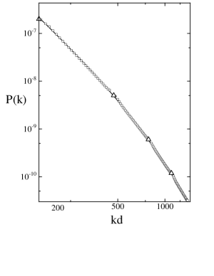
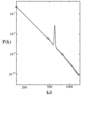
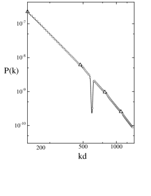
FIG. 3.: The original spectra (the solid curves) and the reconstructed spectra (the boxes and triangles). The left panel shows the case of the double power-law spectrum given by Eq. (44) and the middle and the right panels show the single power-law spectra with a sharp peak ($s=+1$) and a dip ($s=-1$), respectively, given by Eq. (45). The triangles show the locations of the singular points. We stopped the numerical integrations in the vicinity of the singularities when the relative error exceeded 10 %.

FIG. 4.: The CMB angular power spectra for the two initial spectra, Eq. (44) (left panel) and Eq. (45) (right panel). The solid line and the dashed line on the right panel show the case with a peak ($s=+1$) and the case with a dip ($s=-1$), respectively, and the dotted line shows the case without the spiky structure in the initial spectrum. The normalization is arbitrary. Since we have neglected the contribution of baryons to the transfer functions, the acoustic peaks appear less prominent and their locations are shifted to larger $l$. For realistic models with baryons, the acoustic peaks will become more prominent and their locations will shift to smaller $l$. For example, the first peak, which is located at $l\sim 300$ in the figures, will shift to $l\sim 200$.

Finally, it is worthwhile to comment that the presence of the singularities in the differential equation (34) may be regarded as an advantage, since the values of $P(k)$ at the singularities can be estimated without solving the differential equation. In particular, if there is a good reason to believe that the spectrum should be a smoothly varying function, a qualitative feature of the spectrum can be obtained at once. For example, in the case of the double power-law spectrum (44), one can see that the original spectrum can be approximately recovered by simply interpolating between the adjacent triangles shown in Fig. 3.

IV Conclusion

We have considered the problem of reconstructing the initial power spectrum of metric perturbation $P(k)$ from $C_{l}$ data. As a first step, we have investigated a simple case, namely, the Einstein-de Sitter universe with negligible baryons and negligible thickness of the LSS. In this toy model, the observed temperature fluctuations are represented only by the perturbation variables on the LSS and the ISW effect is absent. Then, the relation between the initial spectrum and the angular correlation function is expressed in terms of an integral equation. We have shown that this equation can be transformed to a second order differential equation for $P(k)$. We have found that by forming an appropriate linear combination of the angular correlation function and its derivative, the order of the differential equation can be reduced to the first order. The resulting equation is found to have singularities that come from the acoustic oscillations of photons, hence their presence is inevitable in any cosmological models not restricted to our simple model. Fortunately, however, the presence of these singularities turns out to be not only harmless but rather advantageous. At the singularities the coefficient of $P^{\prime}(k)$ vanishes, and the values of $P(k)$ there can be obtained without solving the differential equation. By plotting the values of $P(k)$, one can obtain a rough estimate of the behavior of the spectrum. Then, to recover the precise features of the spectrum, the rest part of $P(k)$ can be solved with its values at the singularities as the initial values. We have found our method can reproduce the original spectrum with a good accuracy even for a spectrum with a sharp, spiky structure.

The method presented here is applicable only to the Einstein-de Sitter universe in which the ISW effect is negligible. The ISW effect gives an important contribution even in a flat universe model if the cosmological constant is present. Such a model, called the $\Lambda$CDM model is preferred by recent observations[13]. Our next step is to include the ISW effect in our method which is currently under study.

REFERENCES

- [1] M. J. White, D. Scott and J. Silk, Ann. Rev. Astron. Astrophys. 32, 319 (1994); W. Hu, N. Sugiyama and J. Silk, Nature 386, 37 (1997).
- [2] P. J. E. Peebles and J. T. Yu, Astrophys. J. 162, 815 (1970).
- [3] W. Hu and N. Sugiyama, Astrophys. J. 444, 489 (1995); W. Hu and N. Sugiyama, Phys. Rev. D 51, 2599 (1995).
- [4] J. R. Bond et al. Phys. Rev. Lett. 72, 13 (1994); L. Knox, Phys. Rev. D 52, 4307 (1995); G. Jungman, M. Kamionkowski, A. Kosowski and D. N. Spergel, Phys. Rev. D 54, 1332 (1995); J. R. Bond, G. Efstathiou and M. Tegmark, Mon. Not. R. Astron. Soc. 291, L33 (1997); D. J. Eisenstein, W. Hu and M. Tegmark, Astrophys. J. 518, 2 (1999).
- [5] For a review of inflation, see, e.g., A. D. Linde, Particle Physics and Inflationary Cosmology (Harwood, Chur, Switzerland, 1990); K. A. Olive, Phys. Rep. 190, 181 (1990); D. H. Lyth and A. Riotto, Phys. Rep. 314, 1 (1999).
- [6] S. W. Hawking, Phys. Lett. 115B, 295 (1982); A. A. Starobinsky, ibid 117B, 175 (1982); A. H. Guth and S-Y. Pi, Phys. Rev. Lett. 49, 1110 (1982).
- [7] A. D. Linde, Phys. Lett. 158B, 375 (1985); L. A. Kofman and A. D. Linde, Nucl. Phys. B282, 555 (1987); J. Silk and M. S. Turner, Phys. Rev. D 35, 419 (1987); H. M. Hodges and G. R. Blumenthal, Phys. Rev. D. 42, 3329 (1990); J. Yokoyama and Y. Suto, Astrophys. J. 379, 427 (1991); M. Sasaki and J. Yokoyama, Phys. Rev. 744, 970 (1991); A. A. Starobinsky, JETP Lett. 55, 489 (1992); [Pisma Zh. Eksp. Teor. Fiz. 55 (1992) 477]; J. Yokoyama, Astron. Astrophys. 318, 673 (1997); J. Yokoyama, Phys. Rev. D 58, 083510 (1998);59, 107303 (1999); S. M. Leach and A. R. Liddle, Phys. Rev. D 63, 043508 (2001) [arXiv:astro-ph/0010082]; S. M. Leach, M. Sasaki, D. Wands and A. R. Liddle, Phys. Rev. D 64, 023512 (2001) [arXiv:astro-ph/0101406].
- [8] T. Souradeep et. al., astro-ph/9802262; Y. Wang, D. N. Spergel and M. A. Strauss, astro-ph/9812291; Y. Wang, D. N. Spergel and M. A. Strauss, Astrophys. J. 510, 20 (1999); S. Hannestad, Phys. Rev. D 63, 043009 (2001).
- [9] A. Berera and P. A. Martin, Inverse Problems 15, 1393 (1999).
- [10] R. K. Sachs and A. M. Wolfe, Astrophys. J. 147, 73 (1967).
- [11] H. Kodama and M. Sasaki, Prog. Theor. Phys. Supp. 78, 1 (1984); H. Kodama and M. Sasaki, Int. J. Mod. Phys. A 1, 265 (1986); H. Kodama and M. Sasaki, Int. J. Mod. Phys. A 2, 491 (1987).
- [12] J. Silk, Astrophys. J., 151 459 (1968).
- [13] A. G. Riess et al. [Supernova Search Team Collaboration], Astron. J. 116, 1009 (1998) [arXiv:astro-ph/9805201]; S. Perlmutter et al. [Supernova Cosmology Project Collaboration], Astrophys. J. 517, 565 (1999) [arXiv:astro-ph/9812133].