Baryon bias and structure formation in an accelerating universe

Abstract

In most models of dark energy the structure formation stops when the accelerated expansion begins. In contrast, we show that the coupling of dark energy to dark matter may induce the growth of perturbations even in the accelerated regime. In particular, we show that this occurs in the models proposed to solve the cosmic coincidence problem, in which the ratio of dark energy to dark matter is constant. Depending on the parameters, the growth may be much faster than in a standard matter-dominated era. Moreover, if the dark energy couples only to dark matter and not to baryons, as requested by the constraints imposed by local gravity measurements, the baryon fluctuations develop a constant, scale-independent, large-scale bias which is in principle directly observable. We find that a lower limit to the baryon bias $b>0.5$ requires the total effective parameter of state $w_{e}=1+p/\rho$ to be larger than $0.6$ while a limit $b>0.73$ would rule out the model.

I Introduction

The epoch of acceleration which the universe seems to be experiencing rie is commonly regarded as a barren ground for what concerns structure formation. In fact, during an accelerated expansion gravity is unable to win over the global expansion and the perturbations stop growing. Mathematically, this is seen immediately from the equation governing the evolution of the perturbations in the Newtonian approximation in a flat universe:

$$\delta_{c}^{\prime\prime}+\left(1+\frac{H^{\prime}}{H}\right)\delta_{c}^{\prime}-\frac{3}{2}\Omega_{c}\delta_{c}=0$$ (1)

where $H=d\log a/d\tau$ is the Hubble constant in a conformally flat FRW metric $ds^{2}=a^{2}(-d\tau^{2}+\delta_{ij}dx^{i}dx^{j})$, the subscript $c$ stands for cold dark matter (here we neglect the baryons) and the prime represents derivation with respect to $\alpha=\log a$ . When the dark energy field responsible of the acceleration becomes dominant, $\Omega_{c}\to 0$ and the dominant solution of Eq. (1) becomes $\delta_{c}\sim$ const. Only if gravity can overcome the expansion the fluctuations are able to grow. It appears then that to escape the sterility of the accelerated regime is necessary to prevent the vanishing of $\Omega_{c}$.

As it has been shown in ref. wet95 , an epoch of acceleration with a non-vanishing $\Omega_{c}$ can be realized by coupling dark matter to dark energy. In fact, a dark energy scalar field $\phi$ governed by an exponential potential linearly coupled to dark matter yields, in a certain region of the parameter space, an accelerated expansion with a constant ratio $\Omega_{c}/\Omega_{\phi}$ and a constant parameter of state $w_{\phi}$, referred to as a stationary accelerated era. Similar models have been discussed in pav ; dalal . In amtoc2 we showed that in fact the conditions of constant $\Omega_{\phi}$ and $w_{\phi}$ uniquely determine the potential and the coupling of the dark energy field. In this sense, the model we discuss below is the simplest stationary model: any other one must include at least another parameter to modulate the parameter of state. The main motivation to consider a stationary dynamics is that it would solve the cosmic coicidence problem zla of the near equivalence at the present of the dark energy and dark matter densities pav ; bm ; dalal . The stationarity in fact ensures that the two components have an identical scaling with time, at least from some time onward, regardless of the initial conditions. In amtoc it was shown that, by a suitable modulation of the coupling, structure forms before the accelerated era. Further theoretical motivations for coupled dark energy have been put forward in ref. gasp .

As it will be shown below, the coupling has three distinct, but correlated, effects on Eq. (1): first, as mentioned, it gives a constant non-zero $\Omega_{c}$ in the accelerated regime; second, adds to the “friction” $(1+H^{\prime}/H)\delta_{c}^{\prime}$ an extra term which, in general, may be either positive or negative; third, adds to the dynamical term $-\frac{3}{2}\Omega_{c}\delta_{c}$ a negative contribution that enhances the gravity pull.

The dark energy coupling is a new interaction that always adds to gravity (see e.g. wet95 ; dam96 ). The coupling to the baryons is strongly constrained by the local gravity measurements, so that we assume for simplicity that the baryons are in fact not explicitely coupled to the dark energy as suggested in dam and, in the context of dark energy, in ame3 ; bm (of course there remains the gravitational coupling). This species-dependent coupling breaks the equivalence principle, but in a way that is locally unobservable. However, we show that there is an effect which is observable on astrophysical scales and that may be employed to put a severe constraint on the model. In fact, the baryon perturbations grow in the linear regime with a constant, scale-independent, large-scale bias with respect to the dark matter perturbations, that is in principle observable. Although the bias can be either larger or smaller than unity, we find that all the accelerated models require $b<1$ i.e. baryons less clustered than dark matter (sometimes denotes anti-bias). Such a baryon bias would be a direct signature of an explicit dark matter-dark energy interaction, well distinguishable from most other hydrodynamical mechanisms of bias (see e.g. kly ).

II Coupled dark energy

Consider three components, a scalar field $\phi$, baryons and CDM described by the energy-momentum tensors $T_{\mu\nu(\phi)},$ $T_{\mu\nu(b)}$and $T_{\mu\nu(c)}$, respectively. General covariance requires the conservation of their sum, so that it is possible to consider a coupling such that, for instance,

$$T_{\nu(\phi);\mu}^{\mu} = \sqrt{2/3}\kappa\beta T_{(c)}\phi_{;\nu},$$

$$T_{\nu(c);\mu}^{\mu} = -\sqrt{2/3}\kappa\beta T_{(c)}\phi_{;\nu},$$

where $\kappa^{2}=8\pi G$, while the baryons are assumed uncoupled, $T_{\nu(b);\mu}^{\mu}=0$ because local gravity constraints indicate a baryon coupling $\beta_{b}<0.01$ wet95 ; dam96 . Let us derive the background equations in the flat conformal FRW metric. The equations for this model have been already described in amtoc , in which a similar model (but with a variable coupling) was studied. Here we summarize their properties, restricting ourselves to the case in which radiation has already redshifted away. The conservation equations for the field $\phi$, cold dark matter, and baryons, plus the Einstein equation, are

$$\phi^{\prime\prime}+(2+\frac{H^{\prime}}{H})\phi^{\prime}+a^{2}U_{,\phi} = -\sqrt{2/3}\kappa\beta a^{2}\rho_{c},$$

$$\rho^{\prime}_{c}+3\rho_{c} = \sqrt{2/3}\kappa\beta\rho_{c}\phi^{\prime},$$

$$\rho^{\prime}_{b}+3\rho_{b} = 0$$

$$H^{\prime}+\frac{H}{2}\left[1+\kappa^{2}(\frac{1}{2}\phi^{\prime 2}-\frac{a^{2}}{H^{2}}U)\right] = 0$$ (2)

where $U(\phi)=U_{0}e^{-\sqrt{2/3}\mu\kappa\phi}$ . The coupling $\beta$ can be seen as the relative strength of the dark matter-dark energy interaction with respect to the gravitational force. The only parameters of our model are $\beta$ and $\mu$ (the constant $U_{0}$ can always be rescaled away by a redefinition of $\phi$). For $\beta=\mu=0$ we reduce to the standard cosmological constant case, while for $\beta=0$ we recover the Ferreira & Joyce model fer . As shown in ref. wet95 , the coupling we assume here can be derived by a conformal transformation of a Brans-Dicke model, which automatically leaves the radiation uncoupled. To decouple the baryons one needs to consider a two-metric Brans-Dicke Lagrangian as proposed in dam .

The system (2) is best studied in the new variables cop ; ame3 $x=\kappa\phi^{\prime}/\sqrt{6},\quad y=\frac{\kappa a}{H}\sqrt{U/3},$ and $u=\frac{\kappa a}{H}\sqrt{\rho_{b}/3}$ . Then we obtain

$$x^{\prime} =-\frac{1}{2} \left(3-3x^{2}+3y^{2}\right)x-\mu y^{2}+\beta(1-x^{2}-y^{2}-u^{2}),$$

$$y^{\prime} = \mu xy+\frac{1}{2}y\left(3+3x^{2}-3y^{2}\right),$$

$$u^{\prime} = \frac{1}{2}u\left(3x^{2}-3y^{2}\right).$$ (3)

The CDM energy density parameter is obviously $\Omega_{c}=1-x^{2}-y^{2}-u^{2}$ while we also have $\Omega_{\phi}=x^{2}+y^{2},$ and $\Omega_{b}=u^{2}$. The system is subject to the condition $x^{2}+y^{2}+u^{2}\leq 1$.

The critical points of system (3) are listed in Tab. I. We denoted with $w_{e}=1+p_{tot}/\rho_{tot}=1+x^{2}-y^{2}$ the total parameter of state. On all critical points the scale factor expansion is given by $a\sim\tau^{p/1-p}=t^{p}$, where $p=2/(3w_{e})$, while each component scales as $a^{-3w_{e}}$. In the table we also denoted $g\equiv 4\beta^{2}+4\beta\mu+18$, and we used the subscripts $b,c$ to denote the existence of baryons or matter, respectively, beside dark energy. In the same table we report the conditions of stability and acceleration of the critical points, denoting $\mu_{+}=(-\beta+\sqrt{18+\beta^{2}})/2$.

Table 1: Critical points.

Point	$x$	$y$	$u$	$\Omega_{\phi}$	$p$	$w_{e}$	stability	acceleration
$a$	$-\frac{\mu}{3}$	$\sqrt{1-\frac{\mu^{2}}{9}}$	0	1	$\frac{3}{\mu^{2}}$	$\frac{2\mu^{2}}{9}$	$\mu<\mu_{+},\mu<\frac{3}{\sqrt{2}}$	$\mu<\sqrt{3}$
$b_{c}$	$-\frac{3}{2\left(\mu+\beta\right)}$	$\frac{\sqrt{g-9}}{2\left|\mu+\beta\right|}$	$0$	$\frac{g}{4\left(\beta+\mu\right)^{2}}$	$\frac{2}{3}\left(1+\frac{\beta}{\mu}\right)$	$\frac{\mu}{\mu+\beta}$	$\beta>0,\mu>\mu_{+}$	$\mu<2\beta$
$b_{b}$	$-\frac{3}{2\mu}$	$\frac{3}{2\left|\mu\right|}$	$\sqrt{1-\frac{9}{2\mu^{2}}}$	$\frac{9}{2\mu^{2}}$	$\frac{2}{3}$	$1$	$\beta<0,\mu>\frac{3}{\sqrt{2}}$	never
$c_{c}$	$\frac{2}{3}\beta$	0	0	$\frac{4}{9}\beta^{2}$	$\frac{6}{4\beta^{2}+9}$	$1+\frac{4\beta^{2}}{9}$	unstable $\forall\mu\,\beta$	never
$d$	$-1$	0	0	1	$1/3$	2	unstable $\forall\mu\,\beta$	never
$e$	$+1$	0	0	1	$1/3$	2	unstable $\forall\mu\,\beta$	never
$f_{b}$	0	0	1	0	$2/3$	1	unstable $\forall\mu\,\beta$	never

As it can be seen, the attractor $a$ can be accelerated but $\Omega_{c}\to 0$, so that structure cannot grow, as in almost all models studied so far. Therefore, from now on we focus our attention on the global attractor $b_{c}$, the only critical point that may be stationary (i.e. $\Omega_{c}$ and $\Omega_{\phi}$ finite and constant) and accelerated. On this attractor the two parameters $\beta$ and $\mu$ are uniquely fixed by the observed amount of $\Omega_{c}$ and by the present acceleration parameter (or equivalently by $w_{e}=\mu/(\mu+\beta)$ ). For instance, $\Omega_{c}=0.20$ and $w_{e}=0.23$ gives $\mu=3$ and $\beta=10$.

III Differential growth rate

Definining the perturbation variables $\delta=\delta\rho/\rho,\quad\frac{\sqrt{6}}{\kappa}\varphi=\delta\phi,\quad ik^{i}\delta u_{i}/a=\theta H,$ the following conservation equations for CDM, baryons and scalar field in the synchronous gauge for the wavenumber $k$ are derived:

$$\delta^{\prime}_{c} = -\theta_{c}-\frac{1}{2}h^{\prime}-2\beta\varphi^{\prime},$$ (4)

$$\theta^{\prime}_{c} = -\left(1+\frac{H^{\prime}}{H}\right)\theta_{c}+2\beta\left(-\frac{k^{2}}{H^{2}}\varphi+\theta_{c}x\right),$$ (5)

$$\delta^{\prime}_{b} = -\theta_{b}-\frac{1}{2}h^{\prime},$$ (6)

$$\theta^{\prime}_{b} = -\left(1+\frac{H^{\prime}}{H}\right)\theta_{b},$$ (7)

$$\varphi^{\prime\prime} + (2+\frac{H^{\prime}}{H})\varphi^{\prime}+\frac{k^{2}}{H^{2}}\varphi+\frac{1}{2}h^{\prime}x+2\mu^{2}y^{2}\varphi=\beta\Omega_{c}\delta_{c}$$ (8)

Moreover we obtain the Einstein equation

$$h^{\prime\prime}=-(1+\frac{H^{\prime}}{H})h^{\prime}-2\left(12\varphi^{\prime}x-6\mu y^{2}\varphi\right)+3(\delta_{c}\Omega_{c}+\delta_{b}\Omega_{b}).$$ (9)

Now, deriving the $\delta^{\prime}_{c}$ equation we obtain

$$\delta^{\prime\prime}_{c}+\left(1+\frac{H^{\prime}}{H}-2\beta x\right)\delta_{c}^{\prime}+(\frac{4\beta^{2}}{3}-1)\frac{3}{2}\delta_{c}\Omega_{c}-\frac{3}{2}\delta_{b}\Omega_{b} =$$ (10)

$$-6\varphi y^{2}\mu+\left(12+4\beta^{2}\right)\varphi^{\prime}x$$

$$+4\beta(\frac{1}{2}\varphi^{\prime}+\frac{k^{2}}{H^{2}}\varphi+\frac{1}{2}h^{\prime}x+\mu^{2}y^{2}\varphi).$$

In the small-scale Newtonian approximation we can take the limit $k\to\infty$. In Eq. (8) this amounts to neglecting the derivatives of $\varphi$ and the potential term $\mu^{2}y^{2}\varphi$, which gives

$$\frac{k^{2}}{H^{2}}\varphi+\frac{1}{2}h^{\prime}x\approx\beta\Omega_{c}\delta_{c}.$$ (11)

Substituting in Eq. (10) and neglecting again $\varphi^{\prime},\varphi^{\prime\prime}$ and the potential term, we obtain

$$\delta^{\prime\prime}_{c}+\left(1+\frac{H^{\prime}}{H}-2\beta x\right)\delta_{c}^{\prime}-\frac{3}{2}\gamma\delta_{c}\Omega_{c}-\frac{3}{2}\delta_{b}\Omega_{b}=0,$$ (12)

where $\gamma\equiv 1+4\beta^{2}/3,$ and similarly for $\delta_{b}$

$$\delta^{\prime\prime}_{b}+\left(1+\frac{H^{\prime}}{H}\right)\delta_{b}^{\prime}-\frac{3}{2}(\delta_{c}\Omega_{c}+\delta_{b}\Omega_{b})=0.$$ (13)

Eq. (12) corrects the equation given in ref. ame3 , which had a wrong sign (the error gives only a minor effect for the small $\beta$ considered in those papers). In Eq. (12) the differences with respect to Eq. (1) that we mentioned in the introduction appear clearly: the friction term and the dynamical term are modified, and the value of $\Omega_{c}$ is constant along the stationary attractor. On the stationary attractor $\Omega_{b}\to 0$ and Eqs. (12) and (13) can be written as

$$\delta^{\prime\prime}_{c}+\frac{1}{2}\left(4-3w_{e}-4\beta x\right)\delta_{c}^{\prime}-\frac{3}{2}\gamma\Omega_{c}\delta_{c} = 0$$

$$\delta^{\prime\prime}_{b}+\frac{1}{2}\left(4-3w_{e}\right)\delta_{b}^{\prime}-\frac{3}{2}\Omega_{c}\delta_{c} = 0$$

where $x,w_{e}$ and $\Omega_{c}$ are given in Table I as functions of the fundamental parameters $\mu,\beta$ for any critical point. The solutions are $\delta_{c}=a^{m_{\pm}}$and $\delta_{b}=ba^{m_{\pm}}$ where

$$m_{\pm} = \frac{1}{4}\left[-4+3w_{e}+4\beta x\pm\Delta\right]$$ (14)

$$b_{\pm} = 3\Omega_{c}/(3\gamma\Omega_{c}+4\beta xm_{\pm})$$ (15)

where $\Delta^{2}=\left(24\gamma\Omega_{c}+(-4+3w_{e}+4\beta x)^{2}\right)$. The constant $b\equiv\delta_{b}/\delta_{c}\equiv b_{+}$ is the bias factor of the growing solution $m\equiv m_{+}$. The scalar field solution is $\varphi\approx(H_{0}a^{(p-1)/p}/k)^{2}\delta_{c}(\beta\Omega_{c}+mbx)$. For small wavelengths $\varphi$ (which is proportional to $\delta\rho_{\phi}/\rho_{\phi}$ ) is always much smaller than $\delta_{c},\delta_{b}$ at the present time (although it could outgrow the matter perturbations in the future if $p>1$).

The solutions $m_{\pm},b_{\pm}$ apply to all the critical solutions of Table I. Let us now focus on the stationary attractor $b_{c}$. For $\beta=0$ we recover the law $m_{\pm}=\frac{1}{4}\left[-1\pm(24\Omega_{c}+1)^{1/2}\right]$ that holds in the uncoupled exponential case of Ferreira & Joyce fer . Four crucial properties of the solutions will be relevant for what follows: first, the perturbations grow (i.e. $m>0$) for all the parameters that make the stationary attractor stable; second, the baryons are anti-biased (i.e. $b<1$) for the parameters that give acceleration; third, in the $k\gg H$ limit (and in the linear regime), the bias factor is scale independent and constant in time; and fourth, the bias is independent of the initial conditions. Numerical integrations of the full set of equations (4-9) that confirm and illustrate the dynamics are shown in Fig. 1. Notice that, in the future, the perturbations will reenter the horizon because of the acceleration, so that the subhorizon regime in which our solutions are valid will not hold indefinitely.

The species-dependent coupling generates a biasing between the baryon and the dark matter distributions. In contrast, the bias often discussed in literature concerns the distribution only of baryons clustered in luminous bodies kly . To observe the baryon bias one should take into account also the baryons not collapsed in galaxies, e.g in Lyman-$\alpha$ clouds or in intracluster gas. A measure of the biasing of the total baryon distributions is possible in principle but is still largely undetermined. Even taking the extremely simplified approach that the baryon bias coincides with the galaxy bias we are confronted with the problem that the galaxy biasing depends on luminosity and type pea . So we considered only very broad limits to $b$: since the acceleration requires anti-bias, we assume $0.5<b<1$. For a comparison, the likelihood analysis of ref. web gives $b\in(0.8,1.9)$ (for IRAS galaxies, at 99% c.l.), but is restricted to $\Lambda$CDM models with primordial slope $n=1$; other estimations do not exclude anti-bias, and might even require it rines .

In Fig. 2 we show all the various constraints. To summarize, they are: a) the present dark energy density $0.6<\Omega_{\phi}<0.8$; b) the present acceleration ($w_{e}<2/3$, implying $\beta>\mu/2$); c) the baryon bias $1>b>0.5$. On the stationary attractor there is a mapping between the fundamental parameters $\mu,\,\beta$ and the observables $w_{e},\Omega_{\phi}$, so one can plot the constraints on either pair of variables. It turns out that these conditions confine the parameters in the small dark shaded area, corresponding to

$$w_{e}\in(0.59-0.67),$$ (16)

$$or\quad\beta\in(1.1-1.4) \mu\in(2.0-2.6).$$ , (17)

Therefore, the parameters of the stationary attractor are determined to within 20% roughly. It is actually remarkable that an allowed region exists at all. The growth rate $m$ is approximately 0.5 in this region. For $b>0.73$ the possibility of a stationary accelerated attractor able to solve the coincidence problem would be ruled out. If one considers the tighter limit $w_{\phi}<0.4$ for the supernovae Ia given at two sigma in ref. dalal for stationary attractors the allowed region would be further reduced, possibly requiring a lower $b$ to survive.

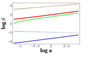
Figure 1: Numerical evolution of the density contrast for a 100 Mpc/$h$ perturbation of dark matter (continuous lines), baryons (dashed lines) and scalar field (dotted lines). Thick lines: $\beta,\mu=1.5,3$ (or $\Omega_{\phi}=0.55,w_{e}=0.67$), resulting in a bias $b\approx 0.3$. Thin lines: $\beta,\mu=0.25,3$ (or $\Omega_{\phi}=0.5,w_{e}=0.92$): here the dark matter and baryon curves are almost indistinguishable since $b\approx 1$.

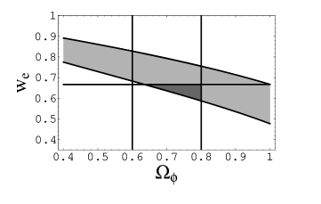
Figure 2: Constraints on the stationary model: below the horizontal line the expansion is accelerated; in the light grey region the bias is between 0.5 and 1; between the vertical lines $\Omega_{\phi}$ is within the observed range. The dark grey region is the surviving parameter space.

IV Conclusions

We have shown that if the universe is experiencing a stationary epoch capable of solving the cosmic coincidence problem then two novel features arise in the standard picture of structure formation. First, a non-zero $\Omega_{c}$ during the accelerated regime allows structure to grow; second, since the baryons have to be uncoupled (or very weakly coupled), the growth is species-dependent, resulting in a constant baryon bias independent of initial conditions. Although there are no direct observations of the baryon bias, the trend is that more massive objects are more biased with respect to the dark matter distribution, so probably the galaxy bias is higher than the total baryon bias. If this is correct, then $b$ can be smaller than unity, as we find to occur for all accelerated models. We find that the bias strongly constrains the existence of a stationary epoch. Putting $b>0.5$, and requiring $0.6<\Omega_{\phi}<0.8$, we get that the two free parameters $\mu$ and $\beta$ are fixed to a precision of 20% roughly, while the effective parameter of state $w_{e}$ is larger than 0.59. A higher bias or a lower $w_{e}$ can easily result in ruling out this class of stationary models. On the other hand, the observation of a constant, scale-independent, large-scale anti-bias would constitute a strong indication in favor of a dark matter-dark energy coupling.

The growth rate $m$ is another observable quantity that can be employed to test the stationarity, for instance estimating the evolution of clustering with redshift. So far the uncertainties of this method are overwhelming (see e.g. magli ) but future data should dramatically improve its validity. The combined test of $b$ and $m$ will be a very powerful test for the dark matter-dark energy interaction. There is also the possibility to compare the resulting power spectrum or cluster abundance with observations, although then we should know exactly when the stationarity begun, and what dynamics preceded it (see e.g. the variable coupling model of ref. amtoc ).

Although we investigated only the simplest stationary model, in which $w_{e}$ is constant (a reasonable assumption over a small redshift range), it is obvious to expect that a similar baryon bias develops whenever there is a species-dependent coupling; this, in turn, is requested to provide stationarity without conflicting with local gravity experiments. Therefore, we conjecture that the baryon bias is a strong test for all stationary dynamics.

References

- (1) A.G. Riess et al. Ap.J., 116, 1009 (1998); S. Perlmutter et al. Ap.J., 517, 565 (1999)
- (2) D. Wands , E.S. Copeland and A. Liddle, Ann. N.Y. Acad. Sci., 688, 647 (1993); C. Wetterich , A& A, 301, 321 (1995); L. Amendola, Phys. Rev. D60, 043501, (1999), astro-ph/9904120
- (3) L. P. Chimento, A. S. Jakubi & D. Pavon, Phys. Rev. D62, 063508 (2000), astro-ph/0005070; W. Zimdahl and D. Pavon, astro-ph/0105479; A. A. Sen & S. Sen, MPLA, 16, 1303 (2001), gr-qc/0103098; T. Chiba Phys. Rev. D64 103503 (2001) astro-ph/0106550
- (4) N. Dalal, K. Abazajian, E. Jenkins, A. Manohar, Phys. Rev. Lett. 87, 141302, 2001
- (5) D. Tocchini-Valentini and L. Amendola, astro-ph/0108143
- (6) I. Zlatev, L. Wang & P.J. Steinhardt, Phys. Rev. Lett. 82 896 (1999).
- (7) R. Bean and J. Magueijo, astro-ph/0007199, Phys. Lett. B517, 177, 2001
- (8) L. Amendola and D. Tocchini-Valentini, astro-ph/0011243, Phys. Rev. D64, 043509, 2001
- (9) M. Gasperini, gr-qc/0105082; A. Albrecht, C.P. Burgess, F. Ravndal, and C. Skordis, astro-ph/0107573; N. Bartolo and M. Pietroni, Phys.Rev. D61 (2000) 023518 ; M. Gasperini, F. Piazza and G. Veneziano, gr-qc/0108016; S. Carroll, Phys. Rev. Lett. 81, 3067 (1998)
- (10) T. Damour, gr-qc/9606079, Proc. 5th Hellenic School of Elementary Particle Physics, 1996; G. Esposito-Farese & D. Polarsky, Phys. Rev. D63, 063504 (2001) gr-qc/0009034
- (11) T. Damour, G. W. Gibbons and C. Gundlach, Phys. Rev. Lett., 64, 123, (1990); T. Damour and C. Gundlach, Phys. Rev. D, 43, 3873, (1991)
- (12) L. Amendola, Phys. Rev. D62, 043511 (2000), astro-ph/9908440; L. Amendola, Phys. Rev. Lett., 86, 196 (2001), astro-ph/0006300
- (13) N. Kaiser, 1984, Ap.J., 284, L9; Bower R.G., Coles P., Frenk C.S. and White S.D.M. 1993 Ap.J. 405, 403; A. Klypin, Lecture at the Summer School "Relativistic Cosmology: Theory and Observations", Italy, Como, May 2000, astro-ph/0005503
- (14) P.G. Ferreira and M. Joyce, Phys. Rev. D58, 2350 (1998)
- (15) E.J. Copeland, A.R. Liddle, and D. Wands, Phys. Rev. D57, 4686 (1997)
- (16) A. Peacock & S.J. Dodds, 1994, MNRAS, 267, 1020; Benoist C. et al. Ap.J. 472, 452 (1996); Norberg et al. 2001, MNRAS, 328, 64
- (17) M. Webster et al. 1998, Ap.J. 509, L65
- (18) K. Rines, M.J. Geller, M.J. Kurtz, A. Diaferio, T.H. Jarrett, J.P. Huchra, astro-ph/0109425
- (19) Magliocchetti, M., Bagla, J. S., Maddox, S. J., & Lahav, O. 2000, MNRAS, 314, 546; Tegmark M., astro-ph/0101354