Properties of the quantum universe in quasistationary states and cosmological puzzles

Abstract

Old and new puzzles of cosmology are reexamined from the point of view of quantum theory of the universe developed here. It is shown that in proposed approach the difficulties of the standard cosmology do not arise. The theory predicts the observed dimensions of nonhomogeneities of matter density and the amplitude of fluctuations of the cosmic background radiation temperature in the Universe and points to a new quantum mechanism of their origin. The large scale structure in the Universe is explained by the growth of nonhomogeneities which arise from primordial quantum fluctuations due to finite width of quasistationary states. The theory allows to obtain the value of the deceleration parameter which is in good agreement with the recent SNe Ia measurements. It explains the large value of entropy of the Universe and describes other parameters.

1 Introduction

The classical cosmology based on the equations of general relativity involving the principles of thermodynamics, hydrodynamics, the plasma theory and the field theory comes across a number of conceptual difficulties known as the problems of standard Big-bang cosmology [1, 2, 3, 4]. These are the problems of singularity, size, age, flatness, total entropy and total mass of the Universe, large-scale structure, dark matter, isotropy of the cosmic microwave background radiation (cmb) and others. The various models were proposed for the solution of these problems. The inflationary model [1, 2] is the most popular one. There are alternative approaches which use the idea that in the early Universe the fundamental constants (velocity of light, gravitational constant, fine-structure constant) had the values different from the modern [5, 6].

The observations of type Ia supernovae (SNe Ia) indicate that our Universe is accelerating [7, 8]. This conclusion which appeared as partly unexpected for the cosmologists a few years ago nowadays practically does not called in question [9]. The concept of a dark energy was proposed for the explanation of this phenomenon [10, 11] and the modern investigations in this field are directed toward filling of this idea with concrete contents [12, 13, 14].

The presence of the cosmological problems points to incompleteness of our knowledge about the Universe. It is generally accepted that the conclusions of classical theory of gravity cannot be extrapolated to the very early epoch. At the Planck scales one must take into account the quantum effects of both matter and gravitational fields.

There cannot be any doubt that our Universe today contains the structural elements which bear the traces of comprehensive quantum processes in preceding epochs. The small cmb anisotropy and observed large-scale structure of the Universe [4] can be given as necessary examples (see below).

The application of basic ideas underlying quantum theory to a system of gravitational and matter fields runs into difficulties of a fundamental character which do not depend on the choice of a specific model. The problem of separation of true degrees of freedom under the construction of quantum gravity becomes of fundamental importance [15]. It is commonly thought that the main reason behind such difficulties is that there is no natural way to define a spacetime event in general covariant theories [16]. At the present time these difficulties are not overcome in the most advanced versions of quantum gravity. Also the quantum gravity cannot rely on experimental data [17]. Therefore it is appropriate to construct the consistent quantum theory within the framework of the simple (toy) exactly soluble cosmological model. As it is well known the model of a homogeneous, isotropic universe (Friedmann-Robertson-Walker model) describes good enough the general properties of our Universe. In this paper we study the model of quantum universe proposed in [18, 19, 20, 21]. It does not meet with the problems mentioned above and comes to the FRW model with positive spatial curvature within the limits of large quantum numbers.

In Sect. 2 we propose the method of removing ambiguities in specifying the time variable in the FRW model by means of modification of the action functional and find the solutions of obtained classical field equations. The Sect. 3 is devoted to the quantum theory for a system of gravitational and matter fields. Here we formulate the equation which is an analog of the Schrödinger equation and turns into the Wheeler-DeWitt one for the minisuperspace model in special case. We concentrate our attention on study of the quantum universe which can be found in a region that is accessible to a classical motion inside the effective barrier formed by the interaction of the fields. We discuss the properties of the wave function of the universe and study the universe in low-lying and highly exited quasistationary states on the basis of exact solution of proposed quantum equation. In this section we calculate the proper dimension of the nonhomogeneities of matter density and the amplitude of fluctuations of the cmb temperature in highly exited state of the universe and propose a new possible quantum mechanism of their origin. The formation and evolution of large scale structure in the universe are considered as an effect of existence of primordial fluctuations due to finite width of quasistationary states. The initially scale-invariant (flat) power spectrum of perturbations and the spectral index are calculated. The results are compared with the observed parameters of our Universe. The flatness of the Universe and the large value of the entropy today receive their natural explanation. The observed accelerated expansion emerges as a macroscopic manifestation of the quantum nature of the Universe.

Throughout the paper the notation Universe (with capital letter U) relates to our Universe, while universe (with small letter u) corresponds to arbitrary cosmological system of considered type.

2 Classical description

2.1 Coordinate condition and basic equations

For simplicity we restrict our study to the case of minimal coupling between geometry and the matter. Considering that scalar fields play a fundamental role both in quantum field theory and in the cosmology of the early Universe we assume that, originally, the Universe was filled with matter in the form of a scalar field $\phi$ with some potential $V(\phi)$. As we shall see the replacement of the entire set of actually existing massive fields by some averaged massive scalar field seems physically justified. We shall consider homogeneous and isotropic universe with positive spatial curvature. Assuming that the field $\phi$ is uniform and the geometry is defined by the Robertson-Walker metric, we represent the action functional in the conventional form

$$S=\int d\eta\,\left[\pi_{a}\,\partial_{\eta}a+\pi_{\phi}\,\partial_{\eta}\phi-\mbox{H}\right].$$ (1)

Here $\eta$ is the time parameter that is related to the synchronous proper time $t$ by the differential equation $dt=N\,a\,d\eta$, where $N(\eta)$ is a function that specifies the time-reference scale, $a(\eta)$ is a scale factor; $\pi_{a}$ and $\pi_{\phi}$ are the momenta canonically conjugate with the variables $a$ and $\phi$, respectively. The Hamiltonian H is given by

$$\mbox{H}=\frac{1}{2}\,N\,\left[-\,\pi_{a}^{2}+\frac{2}{a^{2}}\,\pi_{\phi}^{2}-a^{2}+a^{4}\,V(\phi)\right]\equiv N\,{\cal R},$$ (2)

where the $a$ is taken in units of the length $l=\sqrt{2/3\,\pi}\,l_{Pl}$, $l_{Pl}$ is the Planck length, and $\phi$ in units of $\tilde{\phi}=\sqrt{3/8\,\pi\,G}$. The energy density will be measured in units $(\tilde{\phi}/l)^{2}=(9/16)\,m_{Pl}^{4}$.

The function $N$ plays the role of a Lagrange multiplier, and the variation $\delta S/\delta N$ leads to the constraint equation ${\cal R}=0$. The structure of the constraint is such that true dynamical degrees of freedom cannot be singled out explicitly. In the model being considered, this difficulty is reflected in that the choice of the time variable is ambiguous (the problem of time). For the choice of the time coordinate to be unambiguous, the model must be supplemented with a coordinate condition. When the coordinate condition is added to the field equations, their solution can be found for chosen time variable. However, this method of removing ambiguities in specifying the time variable does not solve the problem of a quantum description. Therefore we shall use another approach and remove the above ambiguity with the aid of a coordinate condition imposed prior to varying the action functional. We will choose the coordinate condition in the form

$$g^{00}\left(\partial_{\eta}T\right)^{2}=\frac{1}{a^{2}}\,,\quad\mbox{or}\quad\partial_{\eta}T=N,$$ (3)

where $T$ is the privileged time coordinate, and include it in the action functional with the aid of a Lagrange multiplier $P$

$$S=\int\!d\eta\,\left[\,\pi_{a}\,\partial_{\eta}a+\pi_{\phi}\,\partial_{\eta}\phi+P\,\partial_{\eta}T-{\cal H}\,\right],$$ (4)

where

$${\cal H}=N\,[\,P+{\cal R}\,]$$ (5)

is the new Hamiltonian. The constraint equation reduces to the form

$$P+{\cal R}=0.$$ (6)

Parameter $T$ can be used as an independent variable for the description of the evolution of the universe. Corresponding canonical equations reduce to the form

$$\partial_{T}a = -\,\pi_{a},\qquad\ \partial_{T}\pi_{a}=\frac{2}{a^{3}}\,\pi^{2}_{\phi}+a-2\,a^{3}V(\phi),$$

$$\partial_{T}\phi = \frac{2}{a^{2}}\,\pi_{\phi},\qquad\partial_{T}\pi_{\phi}=-\,\frac{a^{4}}{2}\,\frac{dV(\phi)}{d\phi},$$

$$\partial_{T}T = 1,\qquad\qquad\partial_{T}P=0.$$ (7)

Integrating the equation for $P$, we obtain $P=E/2$, where $E$ is a constant and the multiplier $1/2$ is introduced for further convenience. The full set of equations for the model in question becomes [18, 19]

$$\left(\partial_{T}a\right)^{2}-\frac{a^{2}}{2}\,\left(\partial_{T}\phi\right)^{2}+U=E,$$ (8)

$$\partial^{2}_{T}\phi+\frac{2}{a}\,\left(\partial_{T}a\right)\left(\partial_{T}\phi\right)+a^{2}\,\frac{dV}{d\phi}=0,$$ (9)

where $U=a^{2}-a^{4}\,V(\phi)$. Equation (8) represents the Einstein equation for the $\left({}^{0}_{0}\right)$ component, while equation (9) is the equation of motion $T^{\mu}_{0;\mu}=0$ for $\phi$, where $T^{\mu}_{\nu}$ is the energy-momentum tensor of the scalar field

$$T^{0}_{0} = \frac{1}{2a^{2}}\left(\partial_{T}\phi\right)^{2}+V,$$

$$T^{1}_{1} = T^{2}_{2}=T^{3}_{3}=-\,\frac{1}{2a^{2}}\left(\partial_{T}\phi\right)^{2}+V,$$

$$T^{\mu}_{\nu} = 0\ \ \mbox{for}\ \ \mu\neq\nu.$$ (10)

From the analysis of the Einstein equations for this model it follows that inclusion of the coordinate condition (3) in the action functional leads to the origin of the additional energy-momentum tensor in these equations

$$\widetilde{T}^{0}_{0} = \frac{E}{a^{4}},\quad\widetilde{T}^{1}_{1}=\widetilde{T}^{2}_{2}=\widetilde{T}^{3}_{3}=-\,\frac{E}{3\,a^{4}},$$

$$\widetilde{T}^{\mu}_{\nu} = 0\ \ \mbox{for}\ \ \mu\neq\nu,$$ (11)

that can be interpreted as the energy-momentum tensor of radiation. In the ordinary units $E$ is measured in $\hbar$. The choice of radiation as the matter reference frame is natural for the case in which relativistic matter (electromagnetic radiation, neutrino radiation, etc.) is dominant at the early stage of Universe evolution. If our Universe were described by the model specified by action functional (4), it would be possible to relate the above radiation at the present era to the cmb.

2.2 Solutions

A feature peculiar to the model in question is that it involves a barrier in the variable $a$ described by the function $U$. This barrier is formed by the interaction of the scalar and gravitational fields. It exists for any form of the positive definite scalar-field potential $V(\phi)$ and becomes impenetrable on the side of small $a$ in the limit $V\rightarrow 0$. In general case ($E\neq 0$) there are two regions accessible to a classical motion: inside the barrier ($a\leq a_{1}$) and outside the barrier ($a\geq a_{2}$), where $a_{1}$ and $a_{2}$ are the turning points ($a_{1}<a_{2}$) specified by the condition $U=E$. The set of equations (8) and (9) determines the $a$ and $\phi$ as the functions of time $T$ at given $V(\phi)$. When the rate at which scalar field changes is much smaller than the rate of universe evolution, i.e. $(\partial_{t}\phi)^{2}\ll 2\,H^{2}$, where $H=\partial_{t}a/a$ is the Hubble constant, and $|\partial_{t}^{2}\phi|\ll|dV/d\phi|$, the equations (8) and (9) become

$$\left(\partial_{T}a\right)^{2}+U=\epsilon,$$ (12)

$$\frac{3}{a}\,H\,\partial_{T}\phi=-\frac{dV}{d\phi},$$ (13)

where $\epsilon$ and $U$ depend parametrically on $\phi$. In the zero-order approximation $\epsilon=E$. The solution to equation (8) can be refined by taking into account a slow variation of the field $\phi$ with the aid of the equation

$$-\,\frac{a^{2}}{2}\,\left(\partial_{T}\phi\right)^{2}+\epsilon(\phi)=E,$$ (14)

where $\epsilon$ stands for a potential term.

The solutions of the equation (13) which determine the scalar field dynamics were studied in the inflationary models [2, 4]. The solution of the equation (12) at fixed value of $\phi$ can be represented in the form

$$a(t) = \left[\frac{1}{2V}+\frac{y}{4V}\ \exp\left\{2\,\sqrt{V}(t-t_{in})\right\}\right.$$ (15)

$$+ \left.\frac{1-4V\epsilon}{4Vy}\ \exp\left\{-\,2\,\sqrt{V}(t-t_{in})\right\}\right]^{1/2},$$

where we denote

$$y=2\,\sqrt{V(\epsilon-\alpha^{2}+\alpha^{4}\,V)}+2V\alpha^{2}-1.$$ (16)

Here $\alpha=a(t_{in})$ gives the initial condition for some instant of time $t=t_{in}$. At $a(0)=0$ and $a(t_{in})=a_{2}$ the corresponding scale factors are given in [18, 19]. The solution (15) shows that in the region $a>a_{2}$ the universe expands in the de Sitter mode from the point $a=a_{2}$, but in the region $a<a_{1}$ it evolves as $a(t)\simeq\left[2\,\sqrt{\epsilon}\,t\right]^{1/2}$ for $2\,\sqrt{V}\,t\ll 1,$ that describes the evolution of the universe which density was dominated by radiation and as $a(t)=a_{1}-\zeta(t)$ with $\zeta(t)\sim t^{2}$ near the point of maximal expansion $a=a_{1}$. The estimations for $a_{1}$ demonstrate that at small enough $V$ the value $a\sim a_{1}$ can reach the modern values of the scale factor in our Universe. So, for the state of the universe with $\epsilon\sim 1/4V$ and $V\sim 10^{-5}$ GeV/cm${}^{3}=6.1\times 10^{-123}$ (the mean matter-energy density in our Universe at the present era) we have $a_{1}\sim\sqrt{1/2V}\sim 10^{61}\sim 10^{28}$ cm.

In the extreme case of $E=0$, where there is no radiation, the region $a\leq a_{1}$ contracts to the point $a=0$, and the expansion can proceed only from the point $a=a_{2}$ and the region $a<a_{2}$ cannot be treated in terms of classical theory. Such models were widely enough studied by many authors (see e.g. [2, 3, 22, 23]).

We concentrate our attention on study of the properties of the universe which is characterized by the nonzero values of $E$ (and $\epsilon$) at the initial instant of time and can be found in a region that is accessible to a classical motion inside the barrier.

The evolution of the universe depends on the initial distribution of the classical field $\phi$ and its subsequent behavior as a function of time. The solutions of the equation (13) for $V\sim\phi^{n}$ give evidence that the $\phi$ decreases with time [2, 3]. From equations (9) and (14), it follows that the inequality $\partial_{T}V+\partial_{T}\epsilon/a^{4}<0$ holds in the expanding universe. If $V$ decreases with time, $\epsilon$ can increase. Let us estimate $\epsilon$ by using the relation $\epsilon\simeq\widetilde{T}^{0}_{0}a^{4}$. In our Universe, with $a\sim 10^{28}$ cm, the main contribution to the radiation-energy density comes from the cmb with energy density $\rho_{\gamma}^{0}\sim 10^{-10}$ GeV/$\mbox{cm}^{3}$. Setting $\widetilde{T}^{0}_{0}=\rho_{\gamma}^{0}$, we find that, at the present era, the result is $\epsilon=\epsilon_{\gamma}\sim 10^{117}\,\hbar$. In the early Universe with $a\sim 10^{-33}$ cm and the Planck energy density we have $\epsilon\sim\hbar$. It indicates that $\epsilon$ should increase in the evolution process. This increase can be explained by a considerable redistribution of energy between the scalar field and radiation at the initial stage of Universe existence. Quantum theory is able to account for this phenomenon in a natural way as spontaneous transition from one quantum state of the universe to another.

Taking into consideration the mechanism of quantum tunneling through the barrier and competing process of the reduction of $V$ with time (which leads to the growth of the barrier $U$ in width and height) allows to reexamine old and new puzzles of cosmology from the point of view of quantum theory.

3 Quantum theory

3.1 Quantization and properties of wave function

In quantum theory, the constraint equation (6) comes to be a constraint on the wave function that describes the universe filled with a scalar field and radiation [18, 19, 20]

$$2\,i\,\partial_{T}\Psi=\left[\partial_{a}^{2}-\frac{2}{a^{2}}\,\partial_{\phi}^{2}-U\right]\Psi\,.$$ (17)

Here the order parameter is assumed to be zero [2, 22, 23]. This equation represents an analog of the Schrödinger equation with a Hamiltonian independent of the time variable $T$. One can introduce a positive definite scalar product $\langle\Psi|\Psi\rangle<\infty$ and specify the norm of a state. This makes it possible to define a Hilbert space of physical states and to construct quantum mechanics for model of the universe being considered.

A solution to equation (17) can be represented in the integral form

$$\Psi(a,\phi,T)=\int_{-\infty}^{\infty}\!dE\,\mbox{e}^{\frac{i}{2}ET}\,C(E)\,\psi_{E}(a,\phi),$$ (18)

where the function $C(E)$ characterizes the $E$ distribution of the states of the universe at the instant $T=0$, while $\psi_{E}(a,\phi)$ and $E$ are, respectively, the eigenfunctions and the eigenvalues for the equation

$$\left(-\,\partial_{a}^{2}+\frac{2}{a^{2}}\,\partial_{\phi}^{2}+U-E\right)\psi_{E}=0.$$ (19)

This equation turns into the famous Wheeler-DeWitt equation for the minisuperspace model [2, 19, 22] in special case $E=0$.

A solution to equation (19) can be represented as

$$\psi_{E}(a,\phi)=\int_{-\infty}^{\infty}\!d\epsilon\,\varphi_{\epsilon}(a,\phi)\,f_{\epsilon}(\phi;E),$$ (20)

where $\varphi_{\epsilon}$ and $\epsilon$ are the eigenfunctions and the eigenvalues of the equation

$$\left(-\,\partial_{a}^{2}+U\right)\varphi_{\epsilon}=\epsilon\,\varphi_{\epsilon}.$$ (21)

For slow-roll potential $V$, when $\left|d\ln V/d\phi\right|^{2}\ll 1$, the $\varphi_{\epsilon}$ describes the universe in the adiabatic approximation and corresponds to continuum states at a fixed value of the field $\phi$. The functions $\varphi_{\epsilon}$ can be normalized to the delta function $\delta(\epsilon-\epsilon^{\prime})$. Their form greatly depends on the value of $\epsilon$. The quantities $f_{\epsilon}(\phi;E)$ can be interpreted as the amplitudes of the probability that the universe is in the state with a given values of $\phi$ and $E$ [20].

Since the potential $U$ has the finite height $U_{max}=1/4V$ and finite width then the quantum tunneling through the region $a_{1}\leq a\leq a_{2}$ of the potential barrier is possible. It results in that stationary states cannot be realized in the region $a\leq a_{1}$. If, however, $V(\phi)\ll 1$, quasistationary states with lifetimes exceeding the Planck time can exist within the barrier. The positions $\epsilon_{n}$ and widths $\Gamma_{n}$ of such states are determined by the solutions to equation (21) for $\varphi_{\epsilon}$ that satisfy the boundary condition in the form of a wave traveling toward greater values of $a$. Let us describe these states.

We choose some value $R>a_{2}$. Then $\varphi_{\epsilon}(a,\phi)$ at fixed $\phi$ can be represented in the form

$$\varphi_{\epsilon}(a)={\cal A}(\epsilon)\,\varphi_{\epsilon}^{(0)}(a)\quad\mbox{for}\quad 0<a<R,$$ (22)

and

$$\varphi_{\epsilon}(a)=\frac{1}{\sqrt{2\pi}}\,\left[\varphi_{\epsilon}^{(-)}(a)-{\cal S}(\epsilon)\,\varphi_{\epsilon}^{(+)}(a)\right]\quad\mbox{for}\quad a>R,$$ (23)

where ${\cal A}(\epsilon)$ and ${\cal S}(\epsilon)$ are the amplitudes depending on $\epsilon$, $\varphi_{\epsilon}^{(0)}$ is the solution that is regular at the point $a=0$, normalized to unity, and weakly dependent on $\epsilon$, while $\varphi_{\epsilon}^{(-)}(a)$ and $\varphi_{\epsilon}^{(+)}(a)$ describe the wave “incident” upon the barrier (the contracting universe) and the “outgoing” wave (the expanding universe) respectively. Beyond the turning points the WKB approximation is valid so that one can write

$$\varphi_{\epsilon}^{(\pm)}(a)=\frac{1}{\sqrt{2}\,(\epsilon-U)^{1/4}}\ \exp\left\{\mp\,i\int_{a_{2}}^{a}\!\sqrt{\epsilon-U}\,da\pm\frac{i\pi}{4}\right\}.$$ (24)

The amplitude ${\cal A}(\epsilon)$ has a pole in the complex plane of $\epsilon$ at $\epsilon=\epsilon_{n}+i\Gamma_{n}$, and for $a<R$ the main contribution to the integral (20) over the interval $-\infty<\epsilon<U_{max}$ comes from the values $\epsilon\approx\epsilon_{n}$. The amplitude ${\cal S}(\epsilon)$ is an analog of the S-matrix [24, 25].

The estimation

$$\left|\varphi_{\epsilon_{n}}\right|_{a<R}\sim\left(\frac{2}{R\,\Gamma_{n}}\right)^{1/2}\,\left|\varphi_{\epsilon_{n}}\right|_{a>R}$$ (25)

shows that at $\Gamma_{n}\ll 1$ the wave function $\varphi_{\epsilon}(a)$ has a sharp peak for $\epsilon=\epsilon_{n}$ and it is concentrated mainly in the region limited by the barrier. If $\epsilon\neq\epsilon_{n}$ then for the maximum value of the function $\varphi_{\epsilon}$ we obtain

$$\left|\varphi_{\epsilon}\right|_{max}^{2}\sim\frac{\Gamma_{n}}{R}\,\frac{\sqrt{\epsilon}}{(\epsilon-\epsilon_{n})^{2}}\,\left|\varphi_{\epsilon}\right|_{a=a_{3}}^{2},$$ (26)

where $U(a_{3})=0$ and $a_{3}\neq 0$. From this it follows that for $\Gamma_{n}\ll 1$ the wave function reaches the great values on the boundary of the barrier, while under the barrier $\varphi_{\epsilon}\sim O(\Gamma_{n})$.

In the limit of an impenetrable barrier, the function $\varphi_{n}=\varphi_{\epsilon_{n}}^{(0)}$ reduces to the wave function of a stationary state with a definite value of $\epsilon_{n}$. During the time interval $\Delta T<1/\Gamma_{n}$ the possibility that the state decays can be disregarded. This corresponds to defining a quasistationary state as that which takes the place of a stationary state when the probability of its decay becomes nonzero [25].

3.2 The universe in low-lying quasistationary states

Calculation of the parameters $\epsilon_{n},\,\Gamma_{n}$ of the quantum state of the universe can be done by both perturbation theory by considering the interaction $a^{4}V(\phi)$ as a small perturbation against $a^{2}$ (in the region $a<a_{1}$ we have $a^{2}V<1$) and direct integration of the equation (21) [18, 19]. Such calculations show that the first level with $\epsilon_{0}=2.62=1.31\,\hbar$ and $\Gamma_{0}=0.31=0.67\,t_{Pl}^{-1}$ emerges at $V=0.08=4.5\times 10^{-2}\,m_{Pl}^{4}$.

In the early universe, the quantity $V(\phi)$ specifies the vacuum energy density. The investigations within inflationary models suggest that the potential $V(\phi(t))$ of the classical scalar field decreases with time. As the potential $V(\phi)$ decreases, the number of quantum states in the prebarrier region increases but the decay probability decreases exponentially. The results of calculations are summarized in the table.

Let us note that the quantum fluctuations of $\phi(t)$ in exponentially expanding universe can result in that the quantity $\phi(t)$ and the potential $V\sim\phi^{n}$ will increase [2, 3]. Then the quantum states of the universe in the prebarrier region cannot form. This case is not interesting for us and it will not be considered.

Table 1: Parameters $\epsilon_{n}$ and $\Gamma_{n}$ for various values of the potential $V$. At $V=5.6\times 10^{-3}\,m_{Pl}^{4}$ there are six levels in the system, three of them are displayed.

$V$ $(m_{Pl}^{4})$	$n$	$\epsilon_{n}$ $(\hbar)$	$\Gamma_{n}$ $(t_{Pl}^{-1})$
$4.5\times 10^{-2}$	0	1.31	$6.7\times 10^{-1}$
$2.8\times 10^{-2}$	0	1.40	$1.3\times 10^{-2}$
$1.7\times 10^{-2}$	0	1.45	$4.3\times 10^{-6}$
	1	3.17	$2.2\times 10^{-2}$
$1.1\times 10^{-2}$	0	1.47	$1.5\times 10^{-10}$
	1	3.30	$2.2\times 10^{-6}$
	2	4.94	$6.5\times 10^{-3}$
$5.6\times 10^{-3}$	0	1.49	$2.2\times 10^{-24}$
	1	3.40	$2.2\times 10^{-19}$
	2	5.26	$2.2\times 10^{-15}$

The calculations demonstrate that the first instants of the existence of the universe (counted off from the moment of formation of first quasistationary state) are especially favorable for its tunneling through the potential barrier $U$. The emergence of new levels results in appearance of competition between the tunneling processes and transitions between the states. In the approximation of a slowly varying field $\phi$, transitions in the system being studied can be considered as those that occur between the states $|n\rangle$ of an isotropic oscillator with zero orbital angular momentum which are induced by the interaction $a^{4}V$. In more strict approach which takes into account the variations of $V(\phi)$ the transitions will be carried out at the expense of the gradient of the potential $V(\phi)$ which follows from the quantization of the equation (6) taking into account the evolution of the field $\phi$ in approximation (13) [24].

Considering the processes of transitions from some initial state $m(T_{0})$ to final state $n(T)$ (including the case $m=n$) and tunneling through the barrier from the final state as independent one can calculate the probability $W_{nm}$ of transition between the states $m$ and $n$ as:

$$W_{nm}\thickapprox\left|\langle\varphi_{n}|\mathcal{U}_{I}|\varphi_{m}\rangle\right|^{2}\,\exp\{-\Gamma_{n}\,\Delta T\},$$ (27)

where $\Delta T=T-T_{0}$ and $\mathcal{U}_{I}$ is the evolution operator in the interaction representation [26]. In the case of two-level system the computation of the total probability of universe decay, $W_{dec}=1-\left(W_{00}+W_{10}\right)$, and the probability $W_{10}$ demonstrates that over the time interval $\Delta T\lesssim 50\,t_{Pl}$, the transitions in the system predominate and only for $\Delta T\sim 10^{2}\,t_{Pl}$ the probability that the universe tunnels through the barrier becomes commensurate with the probability that it undergoes the $0\rightarrow 1$ transition in the prebarrier region (see figure).

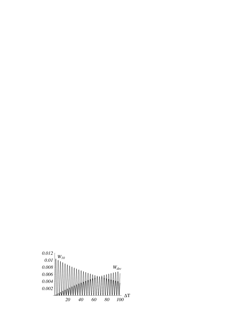
Figure 1: Probabilities $W_{10}$ and $W_{dec}$ versus the time interval $\Delta T=T-T_{0}$ taken in units of the Planck time at $V=1.7\times 10^{-2}\,m_{Pl}^{4}$.

Since the rate at which the level width $\Gamma_{n}$ tends to zero is greater than the rate at which the $V$ decreases, its reduction with time results in that transitions become much more probable than tunnel decays, in which case the former fully determine the evolution of the quantum universe in the prebarrier region. If the universe has not tunneled through the barrier before the potential of the field $\phi$ decreases to a value $V<0.01=5.6\times 10^{-3}\,m_{Pl}^{4}$, a sufficiently large number of levels such that the probabilities of decays from them can be neglected are formed in the system. Calculating the amplitudes of transitions over the time interval $\Delta T$ we find that the $n\rightarrow n+1$ transition is more probable than the $n\rightarrow n-1,\ n+2$ transitions. This means that the quantum universe can undergo transitions to ever higher levels with a nonzero probability. Since the expectation value of the scale factor $\bar{a}_{n}=\langle\varphi_{n}|a|\varphi_{n}\rangle\sim\sqrt{n}$ then it can be concluded that the characteristic size $\bar{a}_{n}$ of the universe that did not undergo a tunnel decay increases as it is excited to higher levels, i.e. the quantum universe being with respect to $a$ in classically accessible region before the turning point $a_{1}$ can evolve so that $\bar{a}_{n}$ will increase with time. This can be interpreted as an expansion of the universe. The probability that, in course of time, the universe will occur in the region $a>a_{2}$ outside the barrier is negligibly small. In the limit $V\rightarrow 0$, the universe is completely locked in the region within the barrier.

The universe in the lowest state with $n=0$ has a “proper dimension” $d\approx\pi\,\bar{a}_{0}\approx 3\times 10^{-33}$ cm, the total matter-energy density $\rho\approx 0.65\,m_{Pl}^{4}$, and the problem of the initial cosmological singularity does not emerge. The classical turning points are $a_{1}\simeq 1.4\times 10^{-33}$ cm and $a_{2}\simeq 2.2\times 10^{-33}$ cm. The value of $a_{1}$ determines the maximal dimension of the universe occurring in the lowest state in prebarrier region, while $a_{2}$ characterizes its initial dimension after tunneling from this state. If a quantum universe tunnels from the states with $n>0$, the dimensions of the region from which tunneling occurs can considerably exceed the Planck length. The constants $E$ and $V$ appearing in the Einstein equations will be determined by the corresponding quantum stage.

Thus it turned out that quantum universe originally filled with a radiation and a matter in form of a scalar field with a potential $V(\phi(t))$ decreasing with time has nonzero probability to evolve remaining in prebarrier region. The expansion here is ensured by the transitions from lower states to higher states by means of interaction between gravitational and scalar fields. The system can be found in the highly excited states with $n\gg 1$ as a result of such evolution. In states with $n\gg 1$ the potential $V\ll 1$ and $\Gamma_{n}\sim 0$. The state of the universe will be characterized by the quantum number $n$ which determines its geometrical properties and new quantum number $s$ responsible for the state of matter.

3.3 Highly excited states

The potential of $\phi$ will be chosen in the form $V(\phi)=(m^{2}/2)\,\phi^{2}$. From the condition $V\ll 1$, it follows that the mass of the field must be constrained by the condition $m\ll m_{Pl}^{2}/|\phi|$. In this case the states of the matter are determined by the solutions of the Schrödinger equation for a harmonic oscillator at given value of $n$ [20]. It describes the oscillations of $\phi$ near the minimum of the potential $V(\phi)$. This process can be interpreted as the production of particles. At $E=0$, a similar mechanism leads to the production of particles by the inflaton field, which is identified with the scalar field $\phi$ [2]. Assuming as before that the $V(\phi)$ is slow-roll potential we find the condition of quantization of $E$

$$E=2N-(2N)^{1/2}(2s+1)m,$$ (28)

where $N=2n+1$, and the values of the quantum number $s$ are restricted by inequality $s+1/2\ll\sqrt{2N^{3}}/m$ which reflects the fact that the mass $m$ of the produced particles is finite. For small $s$ the equality $E\approx 2N$ holds to a high precision, so that the universe is dominated by radiation. A transition from the radiation-dominated universe to the universe where matter (in the form of particles produced by the field $\phi$) prevails occurs when the second term in (28) becomes commensurate with the first one. The physical interpretation of the condition (28) will be considered below.

For the universe with given quantum numbers $n\gg 1$ and $s\gg 1$ the wave function $\psi_{E}$ has the form [20]

$$\psi_{E}(a,\phi)=\varphi_{n}(a)\,f_{ns}(\phi),$$ (29)

where

$$\varphi_{n}(a)=\left(\frac{2}{N}\right)^{1/4}\,\cos\left(\sqrt{2N}\,a-\frac{N\pi}{2}\right),$$

$$f_{ns}(\phi)=\left(\frac{m(2N)^{3/2}}{2(2s+1)}\right)^{1/4}\cos\left(\sqrt{2s+1}\,(2m^{2}N^{3})^{1/4}\,\phi-\frac{s\pi}{2}\right).$$

This wave function is normalized to unity with allowance for the fact that the probability of finding the universe in the region $a>a_{2}$ is negligibly small.

The condition (28) can be rewritten in the terms of “observable” quantities: the cosmic scale factor $\langle a\rangle=\sqrt{N/2}$, where averaging was performed over the state (29), and the total mass of the matter $M=m(s+1/2)$,

$$E=4\langle a\rangle\left[\langle a\rangle-M\right].$$ (30)

The classical universe is characterized by the total energy density $\rho=T_{0}^{0}+\widetilde{T}_{0}^{0}$, where $T_{0}^{0}$ and $\widetilde{T}_{0}^{0}$ are the energy-momentum tensors of the scalar field (10) and radiation (11) respectively. Replacing all quantities by corresponding operators for the quantum universe we set $\rho_{tot}=\langle\rho\rangle$. It gives $\rho_{tot}=\rho_{sub}+\rho_{rad}$, where

$$\rho_{sub}=\frac{193}{12}\,\frac{M}{\langle a\rangle^{3}}\ \quad\mbox{and}\,\quad\rho_{rad}=\frac{E}{\langle a\rangle^{4}}\,.$$ (31)

Here in accordance with the Ehrenfest theorem we assume that expectation value $\langle a\rangle$ follows the laws of classical theory and the expectation values of the functions $T^{0}_{0}$ and $\widetilde{T}^{0}_{0}$ of $a$ can be replaced by the functions of $\langle a\rangle$.

In the case, when $\rho_{sub}\gg\rho_{rad}$ we have $\langle a\rangle=M$. This relation holds to a high precision $\sim 10^{-5}$ in the observed part of our Universe, where $\langle a\rangle\sim 10^{61}\sim 10^{28}$ cm and $M\sim 10^{61}\sim 10^{56}$ g. The quantum numbers of such universe are the following: $n\sim\langle a\rangle^{2}\sim 10^{122}$ and $s\sim\langle a\rangle/m\sim 10^{80}$ taking the proton mass for $m$. The value of $n$ agrees with existing estimates for our Universe, while $s$ is equal to equivalent number of baryons [22, 27].

Thus for the matter-dominant era we have the following relation between $\langle a\rangle$ and $\rho_{sub}$:

$$\langle a\rangle=\left(\frac{193}{12}\,\frac{1}{\rho_{sub}}\right)^{1/2}.$$ (32)

On the other hand in accordance with assumptions made above in the universe with positive spatial curvature in this era the following equality must fulfill [27, 28]

$$\langle a\rangle=\left(\frac{\Omega_{0}}{\Omega_{0}-1}\,\frac{1}{\rho_{sub}}\right)^{1/2},$$ (33)

where $\Omega_{0}=\rho_{sub}/\rho_{c}$ is the matter density in units of the critical density $\rho_{c}$. From (32) and (33) we find $\Omega_{0}=1.07$. That is, the geometry of the universe with $n\gg 1$ and $s\gg 1$ is close to Euclidean geometry (a flat universe).

If one neglects the contribution from the kinetic term of the scalar field ($\pi_{\phi}^{2}=0$) then the corresponding $\Omega_{0}\simeq 0.08$. This value exceeds the contribution from the luminous matter (stars and associated material) [4] and it is close to the value for minimum amount of dark matter required to explain the flat rotation curves of spiral galaxies. Although the potential $V(\phi)$ undergoes only small variations in response to changes in the field $\phi$, the field $\phi$ itself changes fast, oscillating about the point $\phi=0$, so that the approximation in which $\pi_{\phi}^{2}=0$ is invalid. The application of the present model in this approximation would result in the radiation-dominated universe; that is, it would not feature a mechanism capable of filling it with matter after a slow descent of the potential $V(\phi)$ to the equilibrium position, which corresponds to the true vacuum.

It is interesting to find the physical interpretation on (30). Passing on to the ordinary physical units we rewrite it in the form

$$a=G\,M_{tot},$$ (34)

where $M_{tot}=M+U_{rad}$, $U_{rad}\equiv E/2a$. It is easy to see that (34) is the condition of the equality between proper gravitational energy of the thin spherical layer (with the total mass $M_{tot}$) on the sphere with radius $a$ and the sum of energies of particles $M$ and energy of radiation $U_{rad}$. In the modern era $M\sim 10^{80}\,\mbox{GeV}\gg U_{rad}\sim 10^{75}$ GeV. If we extrapolate (34) on Planck era and set $a=l_{Pl}$ then $M_{tot}=m_{Pl}$. For the lowest quantum state we find that $U_{rad}\approx m_{Pl}/2$. Since $s=0$ the parameter $m\approx m_{Pl}$. It means that vacuum energy of the scalar field and the energy of radiation make the comparable contribution to the total energy of universe with $n=0$. In this state the scalar field $|\phi|\approx 0.3\,m_{Pl}$.

3.4 The nonhomogeneities of matter density

The approach developed here makes it possible to obtain realistic estimates for the proper dimensions of nonhomogeneities of matter density, for the amplitude of fluctuations of the cmb temperature and points to a new possible mechanism of their origin, namely by means of finite values of the widths of quasistationary states. For a small, but finite value of the width $\Gamma$ the quasistationary state does not possess a definite value of $\epsilon$. The corresponding uncertainty $\delta\epsilon$ can serve as source of fluctuations of the metric $\delta a$ [20]. By associating $\epsilon+\delta\epsilon$ with the scale factor $a+\delta a$ and by using the solution (15) for $a(0)=0$ we find the amplitude of fluctuations of the scale factor in the form

$$\frac{\delta a}{a}=\frac{1}{4}\,\frac{\delta\epsilon/\epsilon}{1-\tanh(\sqrt{V}t)/2\sqrt{V\epsilon}}\,.$$ (35)

Since $\delta\epsilon\lesssim\Gamma$, the fluctuations $\delta a$ that were generated at the early stage of the evolution of the Universe will take the greatest values. For the lowest quasistationary state with $\epsilon=2.62$, $\delta\epsilon\lesssim 0.31$, $V=0.08$, at $t\sim 1$ we obtain

$$\frac{\delta a}{a}\lesssim 0.04.$$ (36)

Since the dimension of large-scale fluctuations changed in direct proportion $a$, this relation has remained valid up to the present time. For the current value of $a\sim 10^{28}$ cm we find that $\delta a\lesssim 130$ Mpc. On the order of magnitude, the above value corresponds to the scale of superclusters of galaxies. Smaller values of $\delta\epsilon$ are peculiar to quantum states with smaller $V$. The fluctuations $\delta a$ corresponding to them are smaller than (36) and are expected to manifest themselves against the background of the large-scale structure. They can be associated with clusters of galaxies, galaxies themselves, and clusters of stars.

3.5 Fluctuations of the cmb temperature

The energy density of radiation can be expressed as

$$\rho_{rad}=\frac{4\pi^{4}}{30}\,g_{*}\,\mbox{T}^{4},$$ (37)

where T is temperature and $g_{*}$ counts the total number of effectively massless degrees of freedom [1, 2, 4]. Using the relation (31) for $\rho_{rad}$ we obtain

$$E=\frac{4\pi^{4}}{30}\,g_{*}\,\left(a\,\mbox{T}\right)^{4},$$ (38)

where we omit the brackets for simplicity. Leaving the main terms we can write

$$\frac{\delta\mbox{T}}{\mbox{T}}\simeq\frac{1}{4}\,\frac{\delta\epsilon}{\epsilon}-\frac{\delta a}{a}\ .$$ (39)

For $\sqrt{V}\,t\ll 1$ it follows the estimation for the amplitude

$$\frac{\delta\mbox{T}}{\mbox{T}}\simeq\frac{t}{2\sqrt{\epsilon}}\,\frac{\delta a}{a}\ .$$ (40)

For the time $t\sim 10^{5}$ yr corresponding to the instant of recombination of primary plasma (separation of radiation from matter), and for the observed value of $\epsilon=2.6\times 10^{117}\,\hbar$, for (36) we find

$$\frac{\delta\mbox{T}}{\mbox{T}}\lesssim 2.8\times 10^{-5}.$$ (41)

Here $\sqrt{V}\,t\sim 0.7\times 10^{-3}$.

Upon recombination, the fluctuations of the temperature undergo no changes; therefore, measurement of the quantity $\delta\mbox{T}/\mbox{T}$ for the present era furnishes information about the Universe at the instant of last interaction of radiation with matter. The estimate in (41) is in good agreement with experimental data from which the trivial dipole term $\sim 10^{-3}$ caused by the solar system motion was subtracted [29].

3.6 Large scale structure formation

The problem of formation of structure in the Universe is nontrivial in any theoretical scheme [3, 30]. In our approach the quantities (36) and (41) set a restriction from above on possible values of the amplitudes of fluctuations of cosmic scale factor and cmb temperature. In order to describe the power spectrum of density perturbations in the universe and the angular structure of the cmb anisotropies in the context of proposed approach it is necessary to have data about spatial distribution of the fluctuations $\delta\epsilon$. For discussion we shall consider the mechanism of large scale structure formation in the universe based on the fluctuations $\delta\epsilon$ which are distributed in space randomly.

Let us assume that the perturbations $\delta\epsilon$ depend on comoving space coordinates $\mathbf{x}=(x^{1},x^{2},x^{3})$. Below we shall suppose that all perturbations “live” in flat space [31] and $\epsilon$-perturbations $\delta\epsilon(\mathbf{x})$ can be expanded in a Fourier series. According to Sect. 3.1 the state of the universe is characterized by the position $\epsilon$ and width $\Gamma$ of the level (here, for simplicity, the index $n$ which specifies the number of level is omitted). We assume that for given cosmic scale factor $a$ the fluctuations $\delta\epsilon(\mathbf{x})$ have a form of Gaussian distribution in the coordinates $(x^{1},x^{2},x^{3})$ near fixed values $\mathbf{x}_{0}=(x^{1}_{0},x^{2}_{0},x^{3}_{0})$,

$$\delta\epsilon(\mathbf{x})=\frac{\Gamma}{(2\pi)^{3/2}\sigma^{3}}\ \mbox{e}^{-(\mathbf{x}-\mathbf{x_{0}})^{2}/2\sigma^{2}},$$ (42)

where dispersions $\sigma^{2}$ are supposed to be equal for three random values $x^{1},x^{2},x^{3}$. This distribution is normalized as follows

$$\int\!\!d\mathbf{x}\,\delta\epsilon(\mathbf{x})=\Gamma,$$ (43)

where the integral is taken over space. Then the contrast $\delta_{\epsilon}(\mathbf{x})\equiv\delta\epsilon(\mathbf{x})/\epsilon$ averaged over the whole space is

$$\langle\delta_{\epsilon}(\mathbf{x})\rangle_{space}=\frac{\Gamma}{\epsilon}.$$ (44)

For averaged modulus-squared of the contrast $\delta_{\epsilon}(\mathbf{x})$ we have

$$\langle|\delta_{\epsilon}(\mathbf{x})|^{2}\rangle_{space}=\int\!\!\frac{d\mathbf{k}}{(2\pi)^{3}}\,P(k),$$ (45)

where $P(k)=|\delta_{\epsilon}(k)|^{2}$ is the power spectrum and $\delta_{\epsilon}(k)$ is the Fourier component of $\delta_{\epsilon}(\mathbf{x})$. For a homogeneous, isotropic universe $\delta_{\epsilon}(k)$ depends only on wavenumber $k$. From $P(k)$ one can pass to the spectrum

$$\mathcal{P}_{\epsilon}(k)=\frac{k^{3}}{2\pi^{2}}\,P(k),$$ (46)

which is the measure of $\epsilon$-perturbations typical for the scale of wavelengths $\lambda=2\pi/k$ [30, 31, 32]. From (45) we obtain

$$\langle|\delta_{\epsilon}(\mathbf{x})|^{2}\rangle_{space}=\int_{0}^{\infty}\!\frac{dk}{k}\,\mathcal{P}_{\epsilon}(k)=4\pi\int_{0}^{\infty}\!\frac{d\lambda}{\lambda}\,\frac{P(2\pi/\lambda)}{\lambda^{3}}.$$ (47)

Let us introduce the spectral index $n(k)$ of the scalar $\epsilon$-perturbations as follows

$$n(k)=\frac{d\ln P(k)}{d\ln k}.$$ (48)

The Taylor expansion of the spectral index about some fixed wavenumber $k_{0}$

$$n(k)=n(k_{0})+\left(\frac{d\ln n(k)}{d\ln k}\right)_{k_{0}}\ln\frac{k}{k_{0}}+\ldots$$ (49)

gives the following representation for the spectrum

$$P(k)=P(k_{0})\left(\frac{k}{k_{0}}\right)^{n(k_{0})+(1/2)(dn/d\ln k)|_{k_{0}}\ln(k/k_{0})+\ldots}.$$ (50)

It shows that in a power-law approximation a scale-invariant Harrison-Zeldovich (HZ) spectrum [33, 34] corresponds to the case

$$n(k_{0})=1.$$ (51)

The spectrum $P(k)$ can be expressed via the contrast $\delta_{\epsilon}(\mathbf{x})$

$$P(k)=\left|\,\int\!d\mathbf{x}\,\frac{\sin(kx)}{kx}\ \delta_{\epsilon}(\mathbf{x})\right|^{\,2}.$$ (52)

Then the spectral index is

$$n(k)=2\,\left|\frac{\int\!d\mathbf{x}\,\cos(kx)\,\delta\epsilon(\mathbf{x})}{\int\!d\mathbf{x}\,\frac{\sin(kx)}{kx}\,\delta\epsilon(\mathbf{x})}\right|-2.$$ (53)

Substituting (42) into (52) and (53) in the limit of small dispersions $\sigma^{2}$ we find the following simple expressions for the spectrum and the spectral index

$$P(k)=\left(\frac{\Gamma}{\epsilon}\right)^{2}\left|\frac{\sin(kx_{0})}{kx_{0}}\right|^{2},$$ (54)

$$n(k)=2kx_{0}\,|\cot(kx_{0})|-2,$$ (55)

where $x_{0}=|\mathbf{x}_{0}|$. As it is known [31, 32] on the large scale the fundamental spectrum is consistent with HZ slope. In early epoch the equations (51) and (55) define primordial spectrum of $\epsilon$-perturbations with the wavelengths $\lambda_{i}=2\pi/k_{0}^{i}$ equal to

$$\lambda_{1} = 2.9\,x_{0},\ \lambda_{2}=1.4\,x_{0},\ \lambda_{3}=1.3\,x_{0},\ \lambda_{4}=0.82\,x_{0},$$

$$\lambda_{5} = 0.78\,x_{0},\ \lambda_{6}=0.58\,x_{0},\ \lambda_{7}=0.56\,x_{0},\ \mbox{etc}.$$ (56)

In accordance with generally accepted views on mechanisms of formation of visible large scale structure in the Universe [30, 35] one should choose the parameter $x_{0}$ equal to horizon which is determined by the width $\Gamma$ as $x_{0}=1/\Gamma$. Since the primordial spectrum is defined by the discrete set of wavenumbers $k_{0}^{i}$, then the HZ-spectrum itself can be written as sum over all possible roots (56) of transcendental equation (51),

$$P_{HZ}(k)=\sum_{i}P(k_{0}^{i})\,k^{-2}\delta(k-k_{0}^{i}).$$ (57)

Substituting (57) into (47) for the effective value of an amplitude of $\epsilon$-perturbations determined by root mean square of contrast $\delta_{\epsilon}(\mathbf{x})$ we obtain

$$\delta_{\epsilon}^{HZ}=\frac{1}{\sqrt{2}\pi}\left(\sum_{i}P(k_{0}^{i})\right)^{1/2}.$$ (58)

For the lowest state with $\epsilon=2.62,\ \Gamma=0.31$ and the wavelengths (56) from (54) and (58) for the amplitude of $\epsilon$-perturbations of HZ-spectrum we find

$$\delta_{\epsilon}^{Pl}\sim 10^{-2}.$$ (59)

The same estimation can be obtained if one makes a transition from integral in (45) to sum over the vector $\mathbf{k}$ in a cubic lattice with spacing $1/x_{0}=\Gamma$ and then sums over the possible values of $\mathbf{k}$ for HZ-spectrum.

The main contribution to (59) is made by the wavelengths $\lambda_{i}>x_{0}$. The amplitude (59) practically does not change up to the instant of recombination. Indeed, according to (54) we have $\delta_{\epsilon}^{Pl}<(\Gamma/\epsilon)\sim 10^{-1}$. Taking into account that amplitude of $a$-perturbations $\delta a/a$ remains constant during the evolution of the universe (see Sect. 3.4) for the instant of recombination from (35) we find that $\delta_{\epsilon}^{dec}<10^{-1}$ and hence one can consider that the fluctuations (59) also does not change up to the instant of separation of radiation from matter, so that

$$\delta_{\epsilon}^{dec}\sim 10^{-2}.$$ (60)

In order to relate the amplitude of $\epsilon$-perturbations with the density contrast $\delta_{\rho}\equiv\delta\rho/\rho$ the expression for the energy density $\rho=T_{0}^{0}+\widetilde{T}_{0}^{0}$ we rewrite in the form

$$\rho=V+\frac{\epsilon}{a^{4}},$$ (61)

where we have used (14). In the radiation-dominant era $a\simeq[2\sqrt{\epsilon}\,t]^{1/2}$ and

$$\frac{\epsilon}{a^{4}}\simeq\frac{1}{4t^{2}}=\frac{3}{32\pi Gt^{2}}=\rho_{c}.$$ (62)

Here we show in an explicit form the relation between our dimensionless and ordinary units. Since in this era to very high precision $\rho\simeq\rho_{c}$ [2, 3] the potential $V$ in (61) can be neglected. Then at given $a$ for an effective value of energy density perturbations at the instant of recombination we obtain the following estimation

$$\delta_{\rho}^{dec}\approx\delta_{\epsilon}^{dec}\sim 10^{-2}.$$ (63)

After matter-radiation equality, the universe begins a matter-dominated phase and the density contrast $\delta_{\rho}$ increases according to known law $\delta_{\rho}\sim(1+z)^{-1}$, where $z$ is redshift. As far as at the instant of recombination $z=z_{dec}\simeq 10^{3}$ the perturbations (63) guarantee obtaining the value $\delta_{\rho}\sim 1$ by now [3, 33].

Thus in early Universe primordial $\epsilon$-perturbations which are distributed in space randomly can give the necessary value of energy density fluctuation during radiation domination. Nonhomogeneities which arise here can grow up to observed large scale structures (galaxies and their clusters) in the Universe following the standard laws of general relativity. At the same time there is no contradiction between the values (63) and (41). The amplitude of fluctuations $\delta\mbox{T}/\mbox{T}$ according to (40) takes into account the value of $\epsilon$ which has the contribution only from “visible” cmb energy density. Whereas the value (63) effectively includes the contribution from dark matter in the form of scalar field $\phi$ via the parameters $\epsilon$ and $\Gamma$ which are determined from the equation (21).

Primordial fluctuations of $\delta\epsilon(\mathbf{x})$ present one of possible new mechanisms which can contribute to overall picture of formation of large scale structure in the Universe.

It is interesting to clear up the possibility of the description of observed cmb anisotropy on the basis of the $\epsilon$-perturbations. This problem needs detailed study and we shall consider it elsewhere. In Appendix A we give some basic formulas in order to demonstrate in general the possible way of development of our ideas in this direction.

3.7 Entropy

The total entropy $S$ per comoving volume $2\pi^{2}a^{3}$ [1, 2, 4] can be expressed as

$$S=\frac{4\pi^{4}}{45}\,g_{*s}\,\left(a\,\mbox{T}\right)^{3},$$ (64)

where $g_{*s}$ can be replaced by $g_{*}$ for the most of the history of the Universe when all particles species had a common temperature.

From (38) and (64) it follows a simple relation between the $E$ and the total entropy $S$

$$\frac{E}{S}=\frac{3}{2}\,\frac{g_{*}}{g_{*s}}\,a\mbox{T}.$$ (65)

For the adiabatic expansion, $a\mbox{T}=\mbox{const}$, the ratio $E/S$ is conserved. Excluding $a\mbox{T}$ from (65) we obtain the relation,

$$S^{4}=\left(\frac{2}{3}\right)^{5}\frac{\pi^{4}}{5}\,g_{*s}\left(\frac{g_{*s}}{g_{*}}\right)^{3}E^{3}.$$ (66)

In the era with $\mbox{T}\sim 10^{19}$ GeV we have $S\sim 1$, but at present time for $\mbox{T}\sim 10^{-13}$ GeV the entropy $S\sim 10^{88}$. The large value of $E$ today explains the large value of entropy of the Universe.

3.8 Acceleration or deceleration?

Recent measurements [7, 8] indicate that today the Universe is accelerating. Let us note that another possible explanation of the observed dimming of the type Ia supernovae at redshifts $z\sim 0.5$ is an unexpected supernova luminosity evolution [36]. At the present time the first interpretation of observed phenomenon is considered as more preferable.

In terms of classical cosmology the accelerated expansion is described by the negative values of the deceleration parameter

$$q=-\frac{1}{H^{2}}\,\frac{\partial_{t}^{2}a}{a}\ .$$ (67)

In order to agree the experimental data with the theory it was proposed the concept of the dark energy which is nearly smoothly distributed in space. This dark energy component must have negative pressure that overcomes the gravitational self-attraction of matter and causes the accelerated expansion of the Universe. It is commonly assumed that the vacuum energy density in the form of a non-zero cosmological constant or due to a slow-roll scalar field called “quintessence” can be responsible for the dark energy [10, 12, 13].

Let us examine this problem from the point of view of the approach developed in this paper. To this end we rewrite (67) in the form

$$q=1+a\,\frac{\partial_{T}\pi_{a}}{\pi_{a}^{2}}.$$ (68)

Bearing in mind canonical equation for $\partial_{T}\pi_{a}$ from (7) and having differentiated the equation (19) with respect to $a$, we obtain that the derivative $-\,\partial_{T}\pi_{a}$ must be substituted by the quantum mechanical operator

$$\Pi\equiv\frac{1}{2}\left(-\partial_{a}^{2}+\frac{2}{a^{2}}\,\partial_{\phi}^{2}+a^{2}-a^{4}V-E\right)\partial_{a}.$$ (69)

Then according to quantum mechanical principles the quantum analog of deceleration parameter can be calculated as

$$\langle q\rangle=1-\frac{\langle a\,\Pi\rangle}{\langle\pi_{a}^{2}\rangle}\,,$$ (70)

where averaging is performed over states $\psi_{E}$ and it is assumed that offdiagonal matrix elements from $q$ vanish. (This corresponds to the representation of deceleration parameter as a scalar quantity.)

In state with large quantum numbers $n\gg 1$ and $s\gg 1$, for the matter-dominant universe, where $E/4\langle a\rangle^{2}\ll 1$, using the wave function (29) we obtain

$$\langle q\rangle=1-\frac{1}{2}\left[\cos\left(2\pi\langle a\rangle^{2}\right)+\frac{2}{3}\cos\left(\left(2\pi-8\right)\langle a\rangle^{2}\right)\right]\!\!.$$ (71)

The expression in square brackets in (71) which contains two cosines rapidly oscillates with small period $\sim 2l_{Pl}$. Averaging (71) over small interval near some fixed value of $\langle a\rangle^{2}$ we have

$$\overline{\langle q\rangle}=1.$$ (72)

This value can be associated with the deceleration parameter in classical theory. It agrees with the classical conceptions of general relativity about the expansion rate of the Universe in matter-dominated era with zero cosmological constant [27, 28].

The quantity (72) does not take into account the quantum fluctuations of the scale factor

$$\Delta a=\sqrt{\langle a^{2}\rangle-\langle a\rangle^{2}}$$ (73)

that specify root-mean-square deflection of the distribution $|\psi_{E}(a,\phi)|^{2}$ as function of $a$. In this case $\psi_{E}$ represents the wave packet which describes the universe being localized in space $a$ near the expectation value $\langle a\rangle$ with deflection $\Delta a$. We shall show that at certain conditions (parameters of the universe) the fluctuations $\Delta a$ can affect essentially the character of the expansion of the universe. It can provide in particular the accelerated expansion observed nowadays [7, 8].

We shall denote the scale factor taking into account the fluctuations $\Delta a(t)$ as $\widetilde{a}(t)$, while the fluctuations themselves will be associated with quantity $\Delta a(t)=\widetilde{a}(t)-a(t)$, where $a(t)$ is the scale factor without regard for fluctuations of considered type (73). Fixing some instant $t_{0}$ for small intervals $\Delta t=t-t_{0}$ we can write the expansion [27]

$$a(t)=a_{0}\left[1+H_{0}\,\Delta t-\frac{1}{2}\,q_{0}\,H_{0}^{2}\,\Delta t^{2}+\frac{1}{6}\,s_{0}\,H_{0}^{3}\,\Delta t^{3}+\ldots\right],$$ (74)

where $s_{0}\equiv(1/H_{0}^{3})(\partial_{t}^{3}a/a)_{0}$ and subscript $0$ indicates that corresponding values are taken at $t=t_{0}$. The similar series can be written for $\widetilde{a}(t)$ with the Hubble constant $\widetilde{H}_{0}$, the deceleration parameter $\widetilde{q}_{0}$ and $\widetilde{s}_{0}$ calculated with regard to fluctuations. It is natural to assume that the Hubble constant does not depend on the fluctuations (73), i.e. $\widetilde{H}_{0}=H_{0}$. This assumption is based on astrophysical observations which do not record the necessity to modify the classical conception of the Hubble’s law. With regard to this facts from (74) and corresponding series for $\widetilde{a}(t)$ we obtain

$$\left(\frac{\Delta a(t)}{a_{0}}-\frac{\Delta a_{0}}{a_{0}^{2}}\,a(t)\right)\!\!\left(1+\frac{\Delta a_{0}}{a_{0}}\right)^{-1}=-\frac{1}{2}\left(\widetilde{q}_{0}-q_{0}\right)\!H_{0}^{2}\Delta t^{2}+\frac{1}{6}\left(\widetilde{s}_{0}-s_{0}\right)\!H_{0}^{3}\Delta t^{3}+\ldots.$$ (75)

Integrating (75) with respect to $t$ from $t_{1}$ to $t_{0}$ where $|t_{0}-t_{1}|<\mathrm{R}_{c}$, $\mathrm{R}_{c}$ is radius of convergence of the series, we have

$$\left(\frac{\overline{\Delta a}^{t}}{a_{0}}-\frac{\Delta a_{0}}{a_{0}^{2}}\,\overline{a}^{t}\right)\!\left(1+\frac{\Delta a_{0}}{a_{0}}\right)^{-1} = -\frac{1}{6}\left(\widetilde{q}_{0}-q_{0}\right)H_{0}^{2}(t_{0}-t_{1})^{2}$$ (76)

$$- \frac{1}{24}\left(\widetilde{s}_{0}-s_{0}\right)H_{0}^{3}(t_{0}-t_{1})^{3}+\ldots.$$

Here $\overline{a}^{t}$ and $\overline{\Delta a}^{t}$ are the time average of the values $a(t)$ and $\Delta a(t)$ over the interval $[t_{1},t_{0}]$. Using the Einstein equations the parameter $s_{0}$ can be expressed in terms of $q_{0},\ \Omega_{0}$ and pressure $p_{0}$. Assuming that $|\widetilde{\Omega}_{0}-\Omega_{0}|\ll 1$ and $|\widetilde{p}_{0}-p_{0}|\ll 1$, we find

$$\widetilde{s}_{0}-s_{0}=-(\widetilde{q}_{0}-q_{0}).$$ (77)

For the instant of time when the universe is in the state with large quantum numbers, the mean $\langle a\rangle$ may be put to be equal to classical value $a_{0}$. Then according to (73) it is natural to accept

$$\overline{\Delta a}^{t}=\Delta a_{0}=\sqrt{\langle a^{2}\rangle-\langle a\rangle^{2}}\quad\mbox{and}\quad\overline{a}^{t}\approx\frac{a_{0}}{2}.$$ (78)

Then up to discarded terms in (76)

$$\widetilde{q}_{0}=q_{0}-\frac{3}{H_{0}^{2}(t_{0}-t_{1})^{2}}\ \frac{\Delta a_{0}}{a_{0}}\left(1+\frac{\Delta a_{0}}{a_{0}}\right)^{-1}\!\left(1-\frac{1}{4}\,H_{0}(t_{0}-t_{1})\right)^{-1}.$$ (79)

Using wave function (29) from (78) we find that for the state with large quantum numbers the fluctuations

$$\frac{\Delta a_{0}}{a_{0}}=\frac{1}{\sqrt{3}}.$$ (80)

For such fluctuations

$$\widetilde{q}_{0}=q_{0}-\frac{1.1}{H_{0}^{2}(t_{0}-t_{1})^{2}}\ \frac{1}{1-\frac{1}{4}\,H_{0}(t_{0}-t_{1})}.$$ (81)

For numerical estimation in the capacity of $(t_{0}-t_{1})$ one can take the age of the Universe. For modern value $t_{0}-t_{1}=14\ \mbox{Gyr}$ [4] and $H_{0}=65\,\mbox{km}\,\mbox{s}^{-1}\,\mbox{Mpc}^{-1}$ [37, 38] we obtain

$$\widetilde{q}_{0}=q_{0}-1.7.$$ (82)

The parameter $q_{0}$ corresponds to the case when the fluctuations $\Delta a_{0}=0$ and according to (72) it equals to $q_{0}=\overline{\langle q\rangle}=1$. As a result we find

$$\widetilde{q}_{0}=-\,0.7.$$ (83)

This value takes into account the presence of quantum fluctuations of metric and it is in good agreement with SNe Ia observations [7, 8].

Let us note that for used values of Hubble constant and age of the Universe $H_{0}(t_{0}-t_{1})<1$ and convergence of series (76) is not violated (see Appendix B).

Thus, the observed accelerated expansion can be explained without implication of any additional concepts about matter-energy structure of the Universe considering this acceleration as macroscopic manifestation of its quantum nature. In any case unless the whole effect at least a part of it can be caused by quantum fluctuations of considered type.

The represented calculations relate to the universe with large quantum numbers. In preceding epoch the Hubble constant and fluctuations $\Delta a$ took different values. If one assumes, for example, that the relation $H^{2}(t-t_{1})^{2}\sim h^{2}$ holds for earlier instants of time $t$, in epoch with $h\sim 1$ the universe have to be decelerated if the fluctuations $\Delta a<\langle a\rangle/3$. For more accurate calculation of the deceleration parameter of the universe in such states the averaging in (73) must be performed over the wave functions $\psi_{E}$ which take into account that the variables $a$ and $\phi$ in the equation (19) are not separated in general.

4 Concluding remarks

The main constructive element of our model which allows to avoid most of cosmological problems is an idea that $E$ increased during the evolution of the Universe. The quantity $E$ determines the energy-momentum tensor of radiation and can be found as an eigenvalue for the equation (19). The above numerical estimations of the parameters of the quantum universe filled with the radiation and scalar field show that the averaged massive scalar field used instead of the aggregate of real physical fields mainly correctly describes global characteristics of our Universe. It effectively includes visible baryon matter and dark matter. The kinetic energy term of the scalar field provides the modern value of the total energy density of the universe which is very close to the critical value. The status of the field $\phi$ changes as we go over from one stage of universe evolution to another. In the early universe, the field $\phi$ ensures a nonzero value of the vacuum-energy density due to $V(\phi)$ values at which the equation (21) for $\varphi_{\epsilon}(a,\phi)$ admits nontrivial solutions in the form of quasistationary states. In a later era, when the field $\phi$ descends to a minimum of the potential $V(\phi)$ and begins to oscillate about this minimum, it appears to be a source of the particles of some averaged matter filling the visible volume of the universe, which has linear dimensions on the order of $\sim\langle a\rangle$. The galaxies, their clusters, and other structures in the Universe are subject to quantum fluctuations (due to the finite widths of the quasistationary states) that have grown considerably.

The quantum fluctuations which specify the spread of the wave function of the universe in space of scale factor can ensure the accelerated expansion of the universe. In this sense they manifest themselves similar to dark energy. The theory gives the value of the deceleration parameter $q=1$ (the universe is slowing down) for essentially classical cosmological macrosystem and predicts $q\approx-1$ (the universe is speeding up) explaining the accelerated expansion as macroscopic manifestation of quantum nature of the universe.

Acknowledgement

We should like to express our gratitude to Alexander von Humboldt Foundation (Bonn, Germany) for the assistance during the research.

Appendix A

According to general approach (see e.g. [31, 39]) the detailed angular structure of the cmb anisotropy can be characterized by the two-point correlation function

$$C(\vartheta)=\langle\frac{\delta\mbox{T}(\mathbf{e}_{1})}{\mbox{T}}\ \frac{\delta\mbox{T}(\mathbf{e}_{2})}{\mbox{T}}\rangle_{\Omega^{\prime}},$$

where $\vartheta$ is the angle between the directions $\mathbf{e}_{1}$ and $\mathbf{e}_{2}$ in which the anisotropy is observed and the average goes over all points on the celestial sphere separated by an angle $\vartheta$. If one supposes that $\epsilon$-perturbations are distributed in space along the directions $\mathbf{e}$, then according to (35), (39) for $\sqrt{V}t\ll 1$ the fluctuations of temperature in (A1) can be written in the form

$$\frac{\delta\mbox{T}(\mathbf{e})}{\mbox{T}}=-\frac{1}{4}\ \frac{t}{2\sqrt{\epsilon}-t}\ \frac{\delta\epsilon(\mathbf{e})}{\epsilon}.$$

From here it follows that correlation function $C(\vartheta)$ up to multiplier depending on time will be determined by

$$\langle\frac{\delta\epsilon(\mathbf{e}_{1})}{\epsilon}\ \frac{\delta\epsilon(\mathbf{e}_{2})}{\epsilon}\rangle_{\Omega^{\prime}}=\sum_{l=2}^{\infty}Q_{l}^{2}\,P_{l}(\cos\vartheta).$$

Here $P_{l}$ is a Legendre polynomial,

$$Q_{l}^{2}=\frac{1}{4\pi}\sum_{m=-l}^{l}\left|a_{lm}\right|^{2}$$

are the multipole moments and the coefficients $a_{lm}$ are

$$a_{lm}=\int\!d\Omega\,\frac{\delta\epsilon(\mathbf{e})}{\epsilon}\ Y_{lm}^{*}(\mathbf{e}),$$

where $Y_{lm}$ is a spherical harmonic, and the integral is taken over all directions in space. Specifying the form of distribution $\delta\epsilon(\mathbf{e})/\epsilon$ we can calculate the correlation function (A1).

Appendix B

The first omitted term of the series (76) has a form

$$\frac{1}{120}\,\left(\widetilde{r}_{0}-r_{0}\right)H_{0}^{4}\left(t_{0}-t_{1}\right)^{4},$$

where $r_{0}\equiv(1/H_{0}^{4})(\partial_{t}^{4}a/a)_{0}$ and similarly for $\widetilde{r}_{0}$. In order to estimate it we shall suppose as in Sect. 3.8 that energy densities $\rho_{0},\ \widetilde{\rho_{0}}$ and pressures $p_{0},\ \widetilde{p}_{0}$ slightly differ from each other. Then we obtain that ratio

$$\left|\frac{\frac{1}{120}\,\left(\widetilde{r}_{0}-r_{0}\right)H_{0}^{4}\left(t_{0}-t_{1}\right)^{4}}{\frac{1}{24}\,\left(\widetilde{s}_{0}-s_{0}\right)H_{0}^{3}\left(t_{0}-t_{1}\right)^{3}}\right|\approx 0.06.$$

This value must be compared with ratio

$$\left|\frac{\frac{1}{24}\,\left(\widetilde{s}_{0}-s_{0}\right)H_{0}^{3}\left(t_{0}-t_{1}\right)^{3}}{\frac{1}{6}\,\left(\widetilde{q}_{0}-q_{0}\right)H_{0}^{2}\left(t_{0}-t_{1}\right)^{2}}\right|\approx 0.23$$

of first two terms of the series (76). These estimations show that the value $\widetilde{q}_{0}\approx-\,0.7$ can be considered as reliable.

References

- [1] A.H. Guth, Phys. Rev. D23, (1981) 347.
- [2] A.D. Linde, Elementary Particle Physics and Inflationary Cosmology (Harwood, Chur 1990).
- [3] A.D. Dolgov, Ya.B. Zeldovich, and M.V. Sazhin, Kosmologiya rannei vselennoi (Cosmology of the Early Universe) (Mosk. Gos. Univ., Moscow 1988).
- [4] E.W. Kolb and M.S. Turner, Europ. Phys. J. C15, (2000) 125.
- [5] A. Albrecht and J. Magueijo, Phys. Rev. D59, (1999) 043516.
- [6] J.B. Barrow, Phys. Rev. D59, (1999) 043515.
- [7] S. Perlmutter et al., Astrophys. J. 517, (1999) 565; astro-ph/9812133.
- [8] A.G. Riess et al., Astron. J. 116, (1998) 1009; astro-ph/9805201.
- [9] M.S. Turner, in Type Ia Supernovae: Theory and Cosmology, eds J.C. Niemeyer and J.B. Truran (Cambridge University Press, 2000); astro-ph/9904049.
- [10] J.P. Ostriker and P.J. Steinhardt, Nature 377, (1995) 600; astro-ph/9505066.
- [11] N.A. Bahcall, J.P. Ostriker, S. Perlmutter, and P.J. Steinhardt, astro-ph/9906463 (1999).
- [12] R.R. Caldwell, R. Dave, and P.J. Steinhardt, Phys. Rev. Lett. 80, (1998) 1582; astro-ph/9708069.
- [13] K. Benabed and F. Bernardeau, astro-ph/0104371 (2001).
- [14] S.C.C. Ng and D.L. Wiltshire, astro-ph/0107142 (2001).
- [15] R. Arnowitt, S. Deser, and Misner C.W., in Gravitation: An Introduction to Current Research, ed. L. Witten (Wiley, New York 1963), 227.
- [16] K.V. Kuchař and C.G. Torre, Phys. Rev. D43, (1991) 419.
- [17] C.J. Isham, talk given at at GR14 Conference (1995), gr-qc/9510063.
- [18] V.V. Kuzmichev, Ukr. Fiz. J. 43, (1998) 896.
- [19] V.V. Kuzmichev, Yad. Fiz. 62, (1999) 758 [Phys. At. Nucl. (Engl. Transl.) 62, (1999) 708], gr-qc/0002029.
- [20] V.V. Kuzmichev, Yad. Fiz. 62, (1999) 1625 [Phys. At. Nucl. (Engl. Transl.) 62, (1999)] 1524, gr-qc/0002030.
- [21] V.E. Kuzmichev and V.V. Kuzmichev, in Hot Points in Astrophysics (JINR, Dubna, 2000) 67.
- [22] J.B. Hartle and S.W. Hawking , Phys. Rev. D28, (1983) 2960.
- [23] A. Vilenkin, Phys. Rev. D50, (1994) 2581.
- [24] V.V. Kuzmichev, Visnyk Astronomichnoi Shkoly [Astronomical School’s Report] 1, (2000) 64.
- [25] A.I. Baz’, Ya.B. Zel’dovich, and A.M. Perelomov, Scattering, Reactions, and Decays in Nonrelativistic Quantum Mechanics (Israel Program of Sci. Transl., Jerusalem 1966).
- [26] P.A.M. Dirac, The Principles of Quantum Mechanics (Clarendon, Oxford 1958).
- [27] C.W. Misner, K.S. Thorne, and J.A.Wheeler, Gravitation (Freeman, San Francisco 1973).
- [28] S. Weinberg, Gravitation and Cosmology (Wiley, New York 1972).
- [29] G.F. Smoot and D. Scott, Europ. Phys. J. C15, (2000) 145.
- [30] P.J.E. Peebles, The Large-Scale Structure of the Universe (Princeton University Press, Princeton 1980).
- [31] A.R. Liddle and D.H. Lyth, Phys. Rep. 231, (1993) 1.
- [32] D.H. Lyth and A. Riotto, Phys. Rep. 314, (1999) 1.
- [33] R. Harrison, Phys. Rev. D1, (1970) 2726.
- [34] Ya.B. Zeldovich, Astron. Astrophys. 5, (1970) 84.
- [35] Ya.B. Zeldovich and I.D. Novikov, Relativistic Astrophysics, Vol. 2, Structure and Evolution of the Universe (University of Chicago Press, Chicago 1983).
- [36] A.G. Reiss, A.V. Filippenko, W. Li, and B.P. Schmidt, Astron. J. 118, (1999) 2668.
- [37] W.L. Freedman, J.R. Mould, R.C. Kennicutt, and B.F. Madore, in Cosmological Parameters and the Evolution of the Universe (Kyoto, 1998); astro-ph/9801080.
- [38] J.R. Mould et al., Astrophys. J. 529, (2000) 786.
- [39] B. Allen and S. Koranda, Phys. Rev. D50, (1994) 3713.