Abstract

We develop general criteria to construct unified frameworks for inflation and quintessence which employ a unique scalar field to drive both. By using such a minimal theoretical framework we avoid having to fine-tune couplings and mass-scales. In particular the initial conditions for quintessence are already fixed at the end of the inflationary epoch. We provide concrete realizations of the method which meet all inflationary and quintessence requirements, such as the COBE normalization and the resulting spectral index $n\approx 0.97$, which is in excellent agreement with the latest CMB data.

1 Introduction

Recent observations of remote Supernova Ia luminosity curves suggest that the Universe is entering a second phase of accelerated expansion, i.e. a late inflationary period [1]. This is also in agreement with a number of other requirements, which suggest that the Universe at present is dominated by a dark energy component, usually associated with the presence of a non-zero cosmological constant [2]. Results of the latest observations of the Cosmic Microwave Background Radiation (CMBR) [3] indicate that the overall energy density of the Universe corresponds to the critical value of a spatially flat Friedman-Robertson-Walker (FRW) spacetime, successfully predicted by inflationary theory. In such a critical Universe the Cold Dark Matter (CDM) content at present cannot be larger than 35%, leaving the remaining 65% unaccounted for [4]. The remaining energy density is best attributed to a dark energy component of negative pressure. This has resurrected the embarrassing issue of the cosmological constant $\Lambda$ [5], previously assumed to vanish due to an unknown symmetry. The so–called $\Lambda$CDM scenario, which invokes a non-zero $\Lambda$ in order to explain the missing dark energy component, is very appealing due to its simplicity. However, it is highly unpleasant from a theoretical point of view because the required value of the cosmological constant has to be fine tuned to the incredible level of $\Lambda^{2}\sim 10^{-120}M_{P}^{4}$, where $M_{P}$ is the Planck mass [6].

Due to this fact, the idea of a time-variable cosmological “constant” [7] (see also [8]) has become very popular because it can potentially account for the “missing” dark energy in a dynamical way. One realization of a dynamical cosmological constant is achieved with the use of a scalar field $Q$, assumed to dominate with its potential energy density the late-time history of the Universe and drive the latter into accelerated expansion at present. This is the so–called, QCDM scenario. The field $Q$ is referred to as quintessence, the fifth element in addition to Cold Dark Matter, Hot Dark Matter, baryons and photons [9]. Quintessence has inspired a large number of authors (e.g. see [10][11]), who have attempted to derive it using a variety of theoretical frameworks such as string/M theory [12], scalar-tensor gravity [13], brane-worlds and large extra dimensions [14], supersymmetry and supergravity [15][16]. However, it has been soon realized that quintessence has to be fine-tuned in a way similar to $\Lambda$ itself [17]. Indeed, while at present $Q\sim M_{P}$, its mass should be $m_{Q}\sim 10^{-33}$eV! It is clearly not an easy task to achieve such extremely small mass from a potential $V(Q)$ without fine-tuning mass-scales or couplings. Moreover, the introduction of yet again another unobserved scalar field, whose origin is unaccounted for, seems unappealing. Finally, a rolling scalar field introduces another fine-tuning problem, namely that of its initial conditions.

A compelling way to overcome the difficulties and disadvantages of the QCDM scenario is to link it with the rather successful inflationary theory. Linking inflation and quintessence is rather natural because both theories are based on the same idea, namely that the Universe undergoes a phase of accelerated expansion when dominated by the energy density of a scalar field, which slowly rolls down its almost flat potential. The successes of inflationary theory are many. Indeed, inflation provides so far the only solution for the horizon and flatness problems compatible with the cosmological principle [18], while also giving a natural explanation for the formation of Large Scale Structure (LSS) (i.e. the distribution of galactic clusters and superclusters) as well as the amplitude and Doppler peaks of the spectrum of the anisotropies of the CMBR [19]. Finally, the cosmological parameters inferred from present observations are totally consistent with inflationary initial conditions.

Quintessential inflation is achieved by identifying $Q$ with the inflaton field $\phi$. Thus, in such a model, the form of the scalar potential is such that results in two phases of accelerated expansion, one at early and the other at late times. There are several possibilities as for the theoretical origin of this scalar field. For example, supergravity theories provide a natural setting for inflationary models [20] as well as quintessence models (e.g. Copelend et al. or Brax and Martin in [15]). Hence, it is reasonable to adopt such a framework also to model quintessential inflation as suggested here.

The attempt to use inflation to account for the present-day vacuum energy [21] has resulted in relatively few models of quintessential inflation to date [22] - [25]. The rarity of quintessential inflationary models in the literature reflects the fact that the formulation of the required scalar potential is very difficult. Indeed, a successful model of quintessential inflation is subject not only to the requirements of inflation and quintessence, but also to a number of additional considerations. For example, the minimum of the potential (taken to be zero, otherwise there is no advantage over $\Lambda$CDM) must not have been reached yet by the rolling scalar field. This requirement is typically satisfied by potentials, which have their minimum displaced at infinity, $V(\phi\!\to\!\infty)\to 0$, a feature referred to as “quintessential tail”. Thus, quintessential inflation is a non-oscillatory inflationary model [26]. Another requirement is that of a “sterile” inflaton, i.e. the scalar $\phi$ should not couple directly to any fields of the Standard Model (SM). This is necessary in order to avoid the decay of $\phi$ into a thermal bath of SM particles at the end of inflation, since we need $\phi$ to survive until today, as required in order to drive the present late phase of accelerated expansion. An additional advantage of considering a “sterile” inflaton is that one avoids the fine-tuning of the couplings between the inflaton and the SM particles, typical for usual inflationary models, in which these couplings have to be kept small in order to preserve the flatness of the inflationary potential. Moreover, a sterile $\phi$ avoids the violation of the equivalence principle at present, due to the fact that the ultra-light quintessence field would otherwise correspond to a long-range force. Natural candidates for such sterile inflaton are moduli fields, hidden sector and mirror fields, the radion and so on. In the absence of any couplings with SM fields $\phi$ continues its roll-down after the end of inflation, whereas the Universe reheats via the gravitational production of particles at the end of the inflationary period [27][28]. Because gravitational reheating is inefficient the Universe remains $\phi$-dominated after the end of inflation, this time by the kinetic energy of the scalar field [28][29]. This period of kinetic energy domination, however, is terminated quickly and the Universe enters the radiation domination period of the Standard Hot Big Bang (SHBB).

In the models of [22] and [23] the plethora of constraints and requirements which are to be satisfied by quintessential inflation is managed through the use of a multi-branch scalar potential, that is a potential which changes its form while the field moves from the inflationary to the quintessential phase of its evolution. This change is either fixed “by hand” (such as in the toy-model of [22]) or it is the outcome of a phase transition, which is arranged through some interaction of the inflaton with some other scalar fields (as in the case of [23]). Clearly this requires the introduction of additional scalar fields. Moreover, models which involve a phase transition also need many model parameters, couplings and mass scales that have to be tunned correctly to achieve the desired results. Thus, in such models it is difficult to dispense with the fine-tuning problems of quintessence. Still, a remarkable achievement of the phase-transition models of [23] is that they manage to formulate the scalar potential for quintessential inflation in the context of supersymmetry. Another interesting approach is the one of [24], where a large variety of possible choices for the quintessential inflationary potential is generated through a theory of non-minimally coupled gravity. However, the author of [24] is primarily interested in demonstrating the ability of this framework to allow for the construction of many types of successful potentials without actually attempting to construct models with minimal paramater content, although the latter is plausible in this theory. Finally, although rather interesting, recent attempts to model quintessential inflation using brane-world physics [25] cannot avoid fine-tunning problems due to the large number of undetermined free parameters inherent to the brane-environment.

In this paper we develop general criteria and provide concrete realizations of unified frameworks for inflation and quintessence driven by a single scalar field $\phi$. We adopt an alternative approach to the problem and attempt to formulate quintessential inflation in terms of a single-branch scalar potential, which communicates information from the inflationary to the quintessential phase of the scalar field’s evolution. By using such minimal theoretical framework, we avoid introducing additional scalars and minimize the fine-tuning of couplings and mass-scales. For example, the initial conditions for quintessence are already fixed at the end of the inflationary epoch.

Our paper is organized as follows. In Sec. 2 we discuss, in a model–independent way, the main requirements of quintessential inflation, i.e. those that follow from inflation, such as slow–roll, density perturbations and correct amplitude and spectrum of CMBR anisotropies, sufficient reheating for nucleosynthesis, as well as those that follow from quintessence, such as accelerated expansion at present. We also introduce the concepts of frozen and attractor quintessence. In Sec. 3 we present some general criteria required in order to model quintessential inflation, which suggest a preferred choice of the form of the quintessential tail of the scalar potential. Then, in Sec. 4 we present a concrete realization in terms of a specific form of the potential and demonstrate how it meets all the necessary requirements outlined previously in Secs. 2 and 3. Finally, in Sec. 5 we draw our conclusions and provide additional discussion on the method and examples presented. Throughout our paper we use units such that $c=\hbar=1$ in which Newton’s gravitational constant is $G=M_{P}^{-2}$, where $M_{P}=1.22\times 10^{19}$GeV.

2 Quintessential Inflation

2.1 The dynamics of the Universe

The equations of motion for a spatially flat FRW Universe consist of Friedman equation, the energy-momentum conservation condition and Raychadhuri equation, as follows

$$H^{2} = \frac{\rho}{3m_{P}^{2}}$$ (1)

$$d(a^{3}\rho) = -p\,d(a^{3})$$ (2)

$$\frac{\ddot{a}}{a} = -\frac{\rho+3p}{6m_{P}^{2}}$$ (3)

where $m_{P}\equiv M_{P}/\sqrt{8\pi}$ is the reduced Planck mass, $\rho$ and $p$ are the total energy density and pressure of the Universe, $H\equiv\dot{a}/a$ is the Hubble parameter with $a(t)$ being the scale factor of the Universe and the dot denotes derivative with respect to the cosmic time $t$. The content of the Universe is modeled as a number of perfect-fluid components with equations of state $p_{i}=w_{i}\rho_{i}$, so that $\rho=\sum_{i}\rho_{i}$ and $p=\sum_{i}p_{i}$.

For each of these components (2) suggests,

$$\rho_{i}\propto a^{-3(1+w_{i})}$$ (4)

If, during a particular period of the Universe evolution, one of the density components, say $\rho_{D}$, dominates we can identify $\rho\simeq\rho_{D}$ and $p\simeq p_{D}\equiv w_{D}\rho_{D}$ so that, using (1) and (4) we find,,

$$H=\frac{2\,t^{-1}}{3(1+w_{D})} \hskip 28.45274pta\propto t^{{}^{\;\mbox{\footnotesize$\frac{2}{3(1+w_{\!D})}$}}}\hskip 28.45274pt \rho=\frac{4}{3(1+w_{D})^{2}}\Big{(}\frac{m_{P}}{t}\Big{)}^{2}$$ (5)

where $w_{D}\neq-1$. In the case of a cosmological constant domination $\rho_{\Lambda}=m_{P}^{2}\Lambda=$ const. and, from (4) we have $w_{\Lambda}=-1$ so that (1) gives $H^{2}=\frac{1}{3}\Lambda$ and $a\propto\exp(Ht)$, i.e. the Universe undergoes pure de-Sitter inflation.

We will assume that $\Lambda=0$ and the Universe is filled with a background density $\rho_{B}$ comprised by pressureless matter $\rho_{m}$ (including baryons and CDM) with $w_{m}=0$ and radiation $\rho_{\gamma}$ (including relativistic matter) with $w_{\gamma}=1/3$ so that,

$$p_{B}=w_{B}\rho_{B}$$ (6)

where $w_{B}=1/3$ {0} for the radiation {matter} era. We also add to the background a homogeneous scalar field $\phi=\phi(t)$, which can also be treated like a perfect fluid with,

$$\begin{array}[]{lll}\rho_{\phi}\equiv\frac{1}{2}\dot{\phi}^{2}+V(\phi)&\hskip 14.22636pt\mbox{and}&p_{\phi}\equiv\frac{1}{2}\dot{\phi}^{2}-V(\phi)\end{array}$$ (7)

where $V=V(\phi)$ is the scalar potential of $\phi$. From the latter it follows that

$$w_{\phi}=\frac{\dot{\phi}^{2}-2V(\phi)}{\dot{\phi}^{2}+2V(\phi)}$$ (8)

From the above, (3) suggests that the Universe may undergo accelerated expansion only if $\rho_{B}<\rho_{\phi}$ and $w_{\phi}<-\frac{1}{3}$. In order to follow the Universe dynamics during the $\phi$-dominated periods we also need the scalar field equation of motion,

$$\ddot{\phi}+3H\dot{\phi}+V^{\prime}=0$$ (9)

where the prime denotes derivative with respect to $\phi$. Finally, the temperature of the Universe is given by,

$$\rho_{\gamma}=\frac{\pi^{2}}{30}g_{*}T^{4}$$ (10)

where $g_{*}$ is the number of relativistic degrees of freedom, which for the standard model in the early Universe, is $g_{*}=106.75$.

2.2 Inflation

Inflation occurs when the Universe is $\phi$-dominated and the form of $V(\phi)$ is such that the so–called slow–roll parameters

$$\varepsilon\equiv\frac{m_{P}}{\sqrt{6}}\frac{V^{\prime}}{V}\hskip 42.67912pt\eta\equiv\frac{m_{P}^{2}}{3}\frac{V^{\prime\prime}}{V}$$ (11)

satisfy the slow–roll conditions: $|\varepsilon|,|\eta|<1$. In view of these conditions (1) and (9) become,

$$H^{2} \simeq V/3m_{P}^{2}$$ (12)

$$3H\dot{\phi} \simeq -V^{\prime}$$ (13)

In general, during inflation it is useful to express all the relevant quantities as functions of the number of remaining e-foldings until the end of inflation, which is defined as,

$$N\equiv\int^{a_{N}}_{a_{\rm end}}\frac{da}{a}\simeq\int_{\phi_{\rm end}}^{\phi_{N}}\frac{V}{V^{\prime}}\frac{d\phi}{m_{P}^{2}}=\frac{1}{\sqrt{6}}\int_{\phi_{\rm end}}^{\phi_{N}}\frac{d\phi}{\varepsilon\,m_{P}}$$ (14)

Values of $N$ that are of particular interest have to do with length scales that exit the Horizon $N$ e-foldings before the end of inflation and re-enter during the Standard Hot Big Bang (SHBB) at important moments of the evolution of the Universe. Suppose one is interested on the length scale that re-enters the Horizon at time $t_{N}$. The corresponding $N$ is then,

$$N\simeq\ln\Big{(}\frac{T_{N}}{H_{N}}\Big{)}+\ln\Big{(}\frac{H_{\rm end}}{T_{\rm reh}}\Big{)}$$ (15)

where $T_{N}\equiv T(t_{N})$ and $H_{N}=H(t_{N})$ are the temperature and the Hubble parameter of the Universe respectively at the time of re-entry, $T_{\rm reh}$ is the reheating temperature and $H_{\rm end}\equiv H(t_{\rm end})$ is the Hubble parameter at the end of inflation $t_{\rm end}\sim m_{P}/T_{\rm reh}^{2}$.

2.2.1 Density perturbation requirements

One of the big achievements of the inflationary universe idea is that it provides a natural origin for almost scale invariant cosmological density perturbations [20]. The amplitude of the density perturbations is,

$$\frac{\delta\rho}{\rho}\;\simeq\;\left.\frac{H^{2}}{\pi\dot{\phi}}\,\right|_{\rm exit}\simeq-\frac{1}{\sqrt{3}\pi}\frac{V^{3/2}}{m^{3}_{P}V^{\prime}}$$ (16)

where “exit” denotes that the ratio $H^{2}/\pi\dot{\phi}$ should be evaluated when the scale of interest exits the horizon during inflation. The scale of interest is the one which reenters the horizon at the moment of decoupling between matter and radiation $t_{\rm dec}\sim 10^{12}$sec (when the CMBR is emitted) because the corresponding overdensity contrast is constrained by COBE observations. The COBE constraint reeds,

$$\left.\frac{\Delta T}{T}\right|_{\rm dec}\simeq\frac{\delta\rho}{\rho}(N_{\rm dec})\simeq 2\times 10^{-5}$$ (17)

where $N_{\rm dec}$ is the remaining number of e-foldings of inflation when the scale in question exits the horizon.

The spectral index of the overdensity spectrum is defined as,

$$n\equiv 1+\frac{d\ln P_{k}}{d\ln k}$$ (18)

where $k^{-1}\sim He^{N}$ is the relevant scale at the end of inflation and, $(P_{k})^{1/2}\sim\frac{\delta\rho}{\rho}(k)$. After some algebra one finds,

$$n-1\simeq 6(\eta-3\varepsilon^{2})$$ (19)

Large Scale Structure (LSS) and CMBR observations [19] suggest that,

$$|n(N_{c})-1|\leq 0.1$$ (20)

where $N_{c}=N_{\rm dec},N_{\rm eq}$ with $N_{\rm eq}$ being the remaining number of e-foldings when the scale which reenters the horizon at $t_{\rm eq}$ exits the horizon during inflation, where $t_{\rm eq}\sim 10^{11}$sec is the time of equal matter and radiation densities (when the main features of LSS are determined). This requirement is achieved if both the slow–roll conditions are strongly satisfied when $N=N_{c}$ (or if  $3\varepsilon^{2}(N_{c})\approx\eta(N_{c})$ such as in [30]).

2.2.2 Horizon and flatness requirements

The horizon problem is solved if the present horizon scale did exit the horizon during the inflationary period. The e-foldings $N_{H}$ since when this happened are found with the use of (15),

$$N_{H}\simeq\ln(T_{\rm\sc cmb}t_{0})+\ln(\frac{H_{\rm end}}{T_{\rm reh}})$$ (21)

where $T_{\rm\sc cmb}$ is the CMBR temperature at present and $t_{0}$ is the SHBB age of the Universe. Solving the flatness problem requires the total number of e-foldings to be large enough to make $\Omega\leadsto 1$, where $\Omega\equiv\rho/\rho_{c}$, with $\rho_{c}$ being the critical energy density for a spatially flat Universe. This requirement is quantified if we assume an initial $\Omega-1$ value of order unity, in which case we find that the necessary number of inflationary e-foldings is,

$$N_{F}\simeq\frac{1}{2}\Big{[}\ln\Big{(}\frac{t_{\rm eq}}{t_{\rm end}}\Big{)}+\frac{2}{3}\ln\Big{(}\frac{t_{\rm dec}}{t_{\rm eq}}\Big{)}-\ln|\Omega_{\rm dec}-1|\Big{]}$$ (22)

where $\Omega_{\rm dec}\equiv\Omega(t_{\rm dec})$. The above can be evaluated using the results of the CMBR observations [3] which suggest that,

$$|\Omega_{\rm dec}-1|\leq 0.1$$ (23)

Thus, the Horizon and flatness problems are solved if,

$$N_{\rm tot}\geq\mbox{max}\{N_{H},N_{F}\}$$ (24)

Typically the density perturbation requirements are used to evaluate the parameters of an inflationary model whereas the horizon and flatness requirements are constraints on the inflationary initial conditions.

2.3 After the end of inflation

2.3.1 Reheating

In quintessential inflation the inflaton does not decay into a thermal bath of Standard Model particles so that it may survive until today and act as quintessence. To that end $\phi$ does not oscillate around its minimum at the end of inflation but continues to roll-down its potential, violating however, the slow roll conditions, so that inflation is terminated (see Fig. 1). The necessary particle (and entropy) production occurs by gravitational means [27]. Since the gravitationally generated fields have an approximately scale invariant spectrum with amplitude given by the Hawking temperature, we have,

$$T_{\rm reh}\simeq\alpha\left(\frac{H_{\rm end}}{2\pi}\right)$$ (25)

where $\alpha\sim 0.01$ is an efficiency factor [28]. In view of this we have $(H_{\rm end}/T_{\rm reh})=2\pi/\alpha$. Thus, from (15) it is evident that, in the case of gravitational reheating, the number of e-foldings before the end of inflation that corresponds to a length scale that re-enters the Horizon at a particular time $t_{N}$ is independent of the inflationary energy scale and, indeed, of any of the model parameters. The only dependence is on the reheating efficiency factor $\alpha$. Thus, in particular, for the scale of the Horizon today and the scales that re-enter the Horizon at $t_{\rm dec}$ and $t_{\rm eq}$ respectively we find,

$$N_{H} \simeq 69.15-\ln\alpha$$

$$N_{\rm dec} \simeq 66.94-\ln\alpha$$ (26)

$$N_{\rm eq} \simeq 64.27-\ln\alpha$$

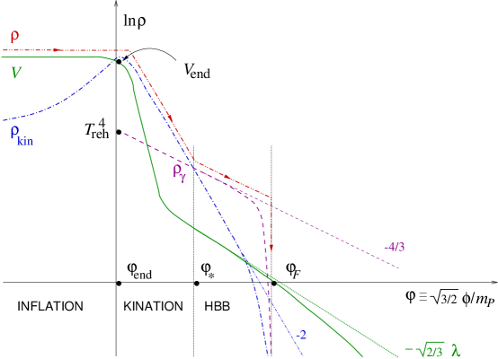
Figure 1: Schematic view of the scalar potential in Quintessential Inflation (solid line). The potential features two flat regions, the inflationary plateau and the quintessential tail. The global minimum is at $+\infty$ so that $V(+\infty)=0$. With such potential inflation is terminated by a drastic reduction of the potential energy density, leading to a rapid roll-down of the scalar field from the inflationary plateau towards the quintessential tail. During inflation $\rho_{\rm kin}=\varepsilon^{2}V$ so that, at the end of inflation ($\varepsilon\simeq 1$), we have $V_{\rm end}\simeq\rho_{\rm kin}(\phi_{\rm end})$. Due to this fact, after the end of inflation, the kinetic energy density of the scalar field $\rho_{\rm kin}$ (dash-dot line) dominates for a brief period the energy density of the Universe. During this kination phase the background energy density $\rho_{B}\simeq\rho_{\gamma}$ (dashed line) reduces less rapidly than $\rho_{\rm kin}$. As a result, even though at the end of inflation $\rho_{\gamma}(\phi_{\rm end})\sim T_{\rm reh}^{4}\ll V_{\rm end}$, beyond a certain value $\phi_{*}$ of the scalar field, the Universe becomes radiation dominated and the Hot Big Bang (HBB) begins. After that the kinetic energy of the scalar filed reduces rapidly to zero (i.e. $\rho_{\rm kin}\rightarrow 0$) and the field (asymptotically) freezes to a value $\phi_{F}$, while the overall density of the Universe $\rho$ (dash-dot-dot line) continues to decrease due to Hubble expansion. In the above figure we have plotted the energy densities of the various components of the Universe, as well as the overall energy density of the Universe, with respect to the dimensionless quantity $\varphi\equiv\sqrt{3/2}\,\phi/m_{P}$. Note that in a logarithmic plot, it is easier to depict the difference of the scaling of the various components of the Universe density. For example, during kination, it can be shown that $t\propto e^{\varphi}$ so that $\rho_{\rm kin}\propto e^{-2\varphi}$ and $\rho_{\gamma}\propto e^{-\frac{4}{3}\varphi}$. Assuming a quasi-exponential quintessential tail of the form given by (57) we have $V\propto e^{-\sqrt{2/3}\,\lambda\varphi}/\varphi^{k}$. Hence, the potential energy density in the above plot falls logarithmicaly away from the pure-exponential case (dotted line). In the HBB era it can be shown that $t\propto(\varphi_{F}-\varphi)^{-2}$ so that $\rho_{\rm kin}\propto(\varphi_{F}-\varphi)^{6}$ and $\rho_{\gamma}\propto(\varphi_{F}-\varphi)^{4}$. Consequently, in the above plot, $\rho_{\rm kin},\rho_{\gamma}\rightarrow 0$ while $\phi\rightarrow\phi_{F}$.

2.3.2 Kination

After the end of inflation the Universe is dominated, for some time, by the kinetic energy of the scalar field. Such a period is refereed to as kination or deflation [28][29]. During this epoch $w_{D}=w_{\phi}=1$ (c.f. (8) ) and, from (4), $\rho_{\rm kin}\equiv\frac{1}{2}\dot{\phi}^{2}\propto a^{-6}$, i.e. the kinetic energy of $\phi$ decreases faster than $\rho_{B}$. Thus, in due time $\rho_{B}$ will catch up with $\rho_{\rm kin}$ and kination will be terminated (see Fig. 1).

From (5) we have $a\propto t^{1/3}$ and $H=1/3t$. In view of this and using, (13) and (25) we find that kination ends at,

$$t_{*}=\big{(}\frac{30}{\pi^{2}g_{*}}\big{)}^{3/2}t_{\rm end}\,\frac{V_{\rm end}^{3/2}}{T_{\rm reh}^{6}}=\frac{1}{9}\Big{(}\frac{6\sqrt{\pi}}{\alpha}\Big{)}^{6}\Big{(}\frac{10}{g_{*}}\Big{)}^{3/2}\frac{m_{P}^{7}}{V_{\rm end}^{2}}$$ (27)

where, in view of (5), $t_{\rm end}=m_{P}/\sqrt{3V_{\rm end}}$ is the time when inflation ends and $V_{\rm end}\equiv V(t_{\rm end})$.

The corresponding temperature is obtained with the use of (5) and (10),

$$T_{*}=\pi\sqrt{\frac{g_{*}}{30}}\,\frac{T_{\rm reh}^{3}}{V_{\rm end}^{1/2}}=\frac{\alpha^{3}}{72\pi^{2}}\sqrt{\frac{g_{*}}{30}}\,\frac{V_{\rm end}}{m_{P}^{3}}$$ (28)

Note that we require $t_{*}$ to be before Big Bang Nucleosynthesis (BBN). Thus,

$$T_{\rm\sc bbn}<T_{*}$$ (29)

where $T_{\rm\sc bbn}\simeq 0.5$ MeV is the temperature at the onset of BBN. Note that, in view of (28), the above constraint provides a lower bound on $V_{\rm end}$.

During kination the scalar field equation of motion (9) is written as,

$$\ddot{\phi}+(\dot{\phi}/t)\simeq 0$$ (30)

Solving we find that the scalar field rolls down until the value,

$$\phi_{*}\equiv\phi(t_{*})\simeq\phi_{\rm end}+\sqrt{6}\,\left[2\,\ln\Big{(}\frac{m_{P}}{V^{1/4}_{\rm end}}\Big{)}+\ln\Big{(}\frac{12\pi}{\alpha^{2}}\mbox{\Large$\sqrt{\frac{30}{g_{*}}}$}\,\Big{)}\right]m_{P}$$ (31)

where $\phi_{\rm end}\equiv\phi(t_{\rm end})$ is the value of $\phi$ at which inflation is terminated.

2.3.3 Hot Big Bang

At the onset of the radiation era $\rho_{\rm kin}$ decreases rapidly as, $\rho_{\rm kin}\propto t^{-3}$ since $a\propto t^{1/2}$. Thus $\dot{\phi}\to 0$ in a short time and the field freezes at a value $\phi_{F}$. Indeed, during the radiation era, $H=1/2t$ and (30) suggests,

$$\phi(t)=\phi_{*}+2\dot{\phi_{*}}t_{*}\Big{(}1-\sqrt{\frac{t_{*}}{t}}\,\Big{)}$$ (32)

where $\dot{\phi}_{*}\equiv\dot{\phi}(t_{*})$ is the value of $\dot{\phi}$ at the onset of radiation domination $t_{*}$. From the above we see that for $t>t_{*}$ the value of $\phi$ approaches a freezing point , $\phi_{F}\simeq\phi_{*}+2\dot{\phi_{*}}t_{*}$,

$\phi_{F}\simeq\phi_{*}+2\dot{\phi_{*}}t_{*}$.

For gravitational reheating, (32) gives,

$$\phi_{F}\simeq\phi_{\rm end}+2\sqrt{\frac{2}{3}}\left[1+\frac{3}{2}\ln\Big{(}\frac{12\pi}{\alpha^{2}}\mbox{\Large$\sqrt{\frac{30}{g_{*}}}$}\,\Big{)}+3\ln\Big{(}\frac{m_{P}}{V_{\rm end}^{1/4}}\Big{)}\right]\,m_{P}$$ (33)

where we have used (31) and that, during kination, $\dot{\phi}=\sqrt{\frac{2}{3}}\,m_{P}/t$.

2.4 Quintessence

2.4.1 Frozen and attractor quintessence

After the freezing of the scalar field its energy density is again $V$-dominated. Thus, its evolution is described by (13), in which, however, $H^{-1}=\frac{3}{2}(1+w_{B})t$ as suggested by (5), because the Universe is now dominated by $\rho_{B}$. The solution of the equation of motion is of the form,

$$f(\phi\mbox{\small$(t)$})-f(\phi_{F})=F(t)$$ (34)

where

$$F(t)\equiv\frac{1}{4}(1+w_{B})t^{2} f(\phi)\equiv-\int^{\prime}\frac{d\phi}{V^{\prime}(\phi)}$$ and (35)

where the prime on the integral means that one should not consider constants of integration.

Thus, the above suggests

$$\phi(t)\simeq\left\{\begin{array}[]{lrl}\phi_{F}&\mbox{when}\hskip 14.22636ptf(\phi_{F})\gg F(t)&\;\mbox{\ Frozen}\\ &&\\ \phi_{\rm atr}(t)&\mbox{when}\hskip 14.22636ptf(\phi_{F})\ll F(t)&\;\mbox{\ Attractor}\end{array}\right.$$ (36)

where $\phi_{\rm atr}(t)$ is the solution of

$$f(\phi)\simeq F(t)\Leftrightarrow\frac{1}{4}(1+w_{B})t^{2}=-\int^{\prime}\frac{d\phi}{V^{\prime}(\phi)}$$ (37)

typically referred to as attractor solution [11]. Because $F(t)$ is a growing function of time we expect that initially the field remains frozen at $\phi_{F}$ until some time later when it unfreezes and starts following the attractor solution (see Fig. 2). This occurs when $V(\phi_{\rm atr})\simeq V(\phi_{F})$ so that, at all times,

$$V(\phi)=\mbox{min}\{V(\phi_{F}),V(\phi_{\rm atr})\}$$ (38)

Note that throughout the quintessential evolution of the scalar field the field’s acceleration $\ddot{\phi}$ is ignored because $\phi$, at most, gently rolls down the “quintessential tail” of its potential. It should be pointed out here that this may not be quite true after unfreezing if the tail is steep. However, as will be explained in 3.1.2, such case is not relevant for successful quintessence.

$\begin{array}[]{cc}\leavevmode\hbox{ \epsfbox{q2.eps}}^{(a)}&\leavevmode\hbox{ \epsfbox{q2a.eps}}^{(b)}\\ &\\ \leavevmode\hbox{ \epsfbox{q2b.eps}}^{(c)}&\leavevmode\hbox{ \epsfbox{q2c.eps}}^{(d)}\end{array}$

Figure 2: Diagrams depicting the behaviour of the energy density of the scalar field $\rho_{\phi}$ (solid line) and the background energy density $\rho_{B}$ (dash-dot line) as a function of the scale factor $a$ after the end of inflation, when $a=a_{\rm end}$ until today, when $a=a_{0}$. After the end of inflation the scalar field continues to dominate the Universe through its kinetic energy, because its energy density is initially much larger than the energy density of the background thermal bath, $V_{\rm end}\gg\rho_{B}(a_{\rm end})\sim T_{\rm reh}^{4}$. However, during kination $\rho_{\phi}$ reduces faster than $\rho_{B}$ and, at $a=a_{*}$, the background density becomes dominant and the Hot Big Bang begins. Soon the kinetic energy of the scalar field is reduced to zero and the field freezes when $a=a_{F}$, after which, its energy density is kept constant and equal to $V_{F}$. The various types of attractor and frozen quintessence are shown depending on the position and steepness of the attractor solution (dashed line). In (a) the attractor meets the frozen field only after the present time, resulting in frozen quintessence and eternal acceleration. In (b) the case of a steep attractor is shown, with slope steeper than the background density. Such an attractor meets the frozen field soon after the end of inflation and renders late $\phi$-domination of the Universe impossible. In (c) the case of the exponential attractor is shown, which mimics the background density and results in a constant ratio between $\rho_{\phi}$ and $\rho_{B}$. Eternal acceleration is avoided in this case. Finally, in (d) the case of a mild attractor is shown, with slope not as steep as the background density. This attractor results in attractor quintessence with eternal acceleration.

2.4.2 Coincidence and acceleration requirements

Accounting for the fact that dark energy seems to begin dominating again today requires,

$$V(\phi_{0})=\Omega_{\phi}\rho_{0}$$ (39)

where $\phi_{0}\equiv\phi(t_{0})$ is evaluated at the present time $t_{0}$ and $\Omega_{\phi}\simeq 0.65$ is the ratio of $\rho_{\phi}(t_{0})$ over the critical density today [4], $\rho_{0}\simeq 10^{-120}m_{P}^{4}$.

Moreover, as mentioned above, in order to explain the current accelerated expansion of the Universe we require, $w_{\phi}<-\frac{1}{3}$. Finally, due to (38), the following constraint should be satisfied,

$$\phi_{0}=\left\{\begin{array}[]{llc}\phi_{F}&&V(\phi_{0})<V(\phi_{\rm atr}\mbox{\small$(t_{0})$})\\ &\Leftrightarrow&\\ \phi_{\rm atr}(t_{0})&&V(\phi_{F})>V(\phi_{0})\end{array}\right.$$ (40)

3 How to model quintessential inflation

Apart from the requirements of inflation and quintessence discussed above, quintessential inflationary models must satisfy some additional generic conditions, such as

• “Sterile” inflaton: It is necessary that the scalar field should not be coupled to the standard model fields so that it cannot decay into them at the end of inflation. This is so in order for the field to survive until today and play the role of quintessence. This is most easily realized by having the scalar field be a gauge singlet.

• Quintessential tail: The scalar field should not have reached the minimum of its potential by the present time because it must have a tiny residual potential energy density today. Thus, the minimum of the potential should be placed rather far from the initial value (probably at infinity). Therefore, the required form of the potential contains two flat regions: the inflationary plateau and the quintessential tail.

Finally, it should be mentioned that, since quintessence is introduced to dispense with the pure cosmological constant $\Lambda$, in quintessential inflation we take $\Lambda=0$ and $V_{\rm min}=0$. A qualitative view of the form of the potential for Quintessential Inflation is shown in Fig. 1. We now give some further insights on quintessential and inflationary evolution that will be useful in developing successful forms of the scalar potential.

3.1 Quintessence attractors and trackers

The quintessential tail requirement results in the existence of attractor solutions, which, when followed by the rolling scalar field, lead to dynamics and general behaviour independent of the initial conditions [11]. These attractor solutions may be a benefit or a hazard as regarding the quintessential requirements. Since the nature of the attractor is decided by the specific form of the potential, constraining the attractor is the first step towards the successful modeling of quintessential inflation.

3.1.1 Tracker solutions

A quintessential attractor solution is referred to as a “tracker” when it is such that it enables and assists attractor quintessence to dominate the Universe at late times. This is achieved by having an attractor which leads to late $\phi$-domination of $\rho_{B}$. As a consequence, when the scalar field begins the attractor phase of its evolution, it will inevitably come to dominate the Universe and play the role of quintessence.

The tracker concept is relevant only in attractor quintessence (see Fig. 2(d) ), since in frozen quintessence (Fig. 2(a) ) the attractor is never reached. As explained above, after kination the field lies frozen with potential energy $V_{F}$ much smaller than $\rho_{B}$ so that the Universe evolves according to the SHBB. In attractor quintessence the attractor solution meets the frozen field before the latter dominates the Universe so that, at the onset of the attractor evolution $V_{\rm atr}<\rho_{B}$. Thus, if the attractor is a tracker the ratio $V_{\rm atr}/\rho_{B}$ should be an increasing function of time (or, equivalently, of $\phi$). From the attractor equation (37) and using also the equation of motion of $\phi$ (13) we find,

$$\frac{m_{P}^{2}}{3(1+w_{B})}\Big{(}\frac{V_{\rm atr}}{\rho_{B}}\Big{)}=-V\int^{\prime}\frac{d\phi}{V^{\prime}}$$ (41)

Taking the time derivative of the above we find that the criterion for a tracker attractor is

$$\frac{d}{dt}\Big{(}\frac{V_{\rm atr}}{\rho_{B}}\Big{)}\geq 0\Leftrightarrow V\geq(V^{\prime})^{2}\int^{\prime}\frac{-dV}{(V^{\prime})^{2}}$$ (42)

Similarly, it can be shown that

$$\Gamma\equiv\frac{VV^{\prime\prime}}{(V^{\prime})^{2}}\geq 1\Leftrightarrow\frac{d^{2}}{dt^{2}}\Big{(}\frac{V_{\rm atr}}{\rho_{B}}\Big{)}\geq 0$$ (43)

which is usually enough for the kind of potentials used in quintessence [11]. The case of equality in the above corresponds to potentials with exponential quintessential tail [16][31] and is the limiting case of the tracker solution. As we will discuss below, tracker solutions exist only for potentials with tails of slope milder than that of the exponential tail.

3.1.2 Attractors and slope

The behaviour of the attractor is strongly related to the slope of the quintessential tail of the potential. This can be demonstrated as follows. Derivating (41) with respect to $\phi$ and using also (11) we obtain,

$$\frac{d(1/V_{\rm atr})}{d(1/\rho_{B})}=\frac{2\varepsilon^{2}}{1+w_{B}}$$ (44)

Let us parametrize the behaviour of $\varepsilon(V)$ around the region of $V$ of interest (the quintessential tail) as a power-law,

$$\varepsilon^{2}\equiv C\Big{(}\frac{1}{V}\Big{)}^{q}$$ (45)

where $C$ is a positive constant. The actual value of $\varepsilon^{2}(V\to 0)$ depends on the slope since, $\varepsilon^{2}\propto(V^{\prime})^{2}/V^{2}$ and $V^{\prime}\to 0$ as $V\to 0$. For the exponential slope $\varepsilon^{2}$=const.$>0$. For steeper slopes $(V^{\prime})^{2}$ is larger than the exponential case and thus, $\varepsilon^{2}(V\!\to\!0)\to+\infty$, whereas for milder slopes $(V^{\prime})^{2}$ is smaller than the exponential case so that $\varepsilon^{2}(V\!\to\!0)\to 0$. Thus, in (45) we may consider,

$$\begin{array}[]{rl}q>0&{\rm steep}\\ q=0&{\rm exp}\\ q<0&{\rm mild}\end{array}$$ (46)

Inserting (45) into (44) we find,

$$\frac{V_{\rm atr}}{\rho_{B}}=\frac{(1+w_{B})V^{q}}{2C(1-q)}\propto\Big{(}\frac{1}{V}\Big{)}^{-q}$$ (47)

From the above it is evident that for quintessential-tail with steep {mild} slope $V_{\rm atr}$ reduces with time faster {slower} than $\rho_{B}$. This means that, in the mild case the attractor is such that $V_{\rm atr}$ approaches the background density and, therefore, it is a tracker. In the steep case, however, if the attractor evolution begins, there is no chance that the scalar field will come to dominate the Universe and, therefore, such a case cannot result in quintessential evolution. Thus, for potentials with steeper than exponential tails only frozen quintessence is, in principle, possible.

One can imagine that, even if the onset of the steep attractor is disastrous for quintessence, a steep-tail model may still be acceptable in the case of frozen quintessence with the steep attractor beginning after today. However, it turns out that a steep attractor begins very soon after the end of inflation, which renders frozen quintessence in this case also impossible to attain. This can be understood as follows. From (44) after some trivial algebra we get

$$\frac{1}{2}\frac{d}{d(\ln t)}\Big{(}\frac{\rho_{B}}{V_{\rm atr}}\Big{)}=\frac{2\varepsilon^{2}}{1+w_{B}}-\frac{\rho_{B}}{V_{\rm atr}}$$ (48)

where we also used $\rho_{B}\propto t^{-2}$. In the steep case, before the cross-over of $V_{\rm atr}$ and $\rho_{B}$, we have $V_{\rm atr}\gg\rho_{B}$. Also, in this case $\varepsilon^{2}>1$. Thus, one can ignore the last term of (48) and obtain,

$$\frac{\rho_{B}}{V_{\rm atr}}\simeq\int\frac{4\varepsilon^{2}d(\ln t)}{1+w_{B}}$$ (49)

The above suggests that, because $\varepsilon^{2}$ is very large, the time required for the cross-over is small. Indeed, considering that in such little time $\varepsilon^{2}$ does not change much, we may estimate the cross-over time as,

$$t_{\times}\simeq t_{\rm end}\exp\Big{[}\frac{1}{4}(1+w_{B})\varepsilon^{-2}\Big{]}\sim t_{\rm end}$$ (50)

Thus, we see that the steep-tail attractor begins very soon after the end of inflation and, therefore, one cannot achieve frozen quintessence. The above are illustrated in Fig. 2(b).

It should be noted here that, for steep quintessential tails the $\ddot{\phi}$ term in the equation of motion cannot be ignored. The action of this term intensifies the rapid roll of the field and steepens the attractor even more.

3.1.3 The exponential tail

The exponential tail is the interface between steep and mild slopes. In this case $\varepsilon^{2}=$ const. and (41) gives,

$$\frac{\rho_{B}(t)}{V_{\rm atr}(t)}=\frac{2\varepsilon^{2}}{1+w_{B}}={\rm constant}$$ (51)

Therefore, we see that the scalar field attractor mimics the behaviour of the background matter and evolves as $V_{\rm atr}\propto t^{-2}$.

The exponential tail is also marginally affected by the $\ddot{\phi}$ term in the equation of motion of the scalar field. If this term is also taken into account the above equation becomes,

$$\frac{\rho_{B}(t)}{V_{\rm atr}(t)}=\frac{4\varepsilon^{2}}{1-w_{B}^{2}}={\rm constant}$$ (52)

It is evident that the $\ddot{\phi}$ term is insignificant for milder slopes, where slow–roll conditions are truly satisfied.

Since the attractor solution breaks down when $\rho_{B}\sim V_{F}$ we see that for frozen quintessence we must require,

$$\frac{V_{\rm atr}}{\rho_{B}}>1\Leftrightarrow\varepsilon^{2}<\frac{1}{4}(1-w_{B}^{2})$$ (53)

If the above is violated we have attractor quintessence. In this case we have $V_{\rm atr}\propto\rho_{B}\propto t^{-2}$. Also, using (1) and the field equation (13) we find, $\rho_{\rm kin}\equiv\frac{1}{2}\dot{\phi}^{2}=\varepsilon^{2}V_{\rm atr}^{2}/\rho_{B}\propto t^{-2}$. Thus, in overall $\rho_{\phi}=\rho_{\rm kin}+V_{\rm atr}\propto t^{-2}$, or equivalently, $\rho_{\phi}/\rho_{B}=$ constant [16]. This, in view of (4), implies that $w_{\phi}=w_{B}\geq 0$. Therefore, in attractor quintessence an exponential tail cannot lead to acceleration. Moreover, in this case, because the attractor solution is such that $V_{\rm atr}<\rho_{B}$ at all times, the scalar field never comes to dominate the Universe but remains a constant fraction of the overall density (see Fig. 2(c) ). Therefore, if the scalar field were to account for the dark energy component of the late-time Universe then, at present, we should demand that,

$$V_{\rm atr}\mbox{\raisebox{-3.87495pt}{~{}$\stackrel{{\scriptstyle\mbox{$<$}}}{{\sim}}$~{}}}\rho_{B}$$ (54)

meaning that $V_{\rm atr}$ should be very close but not larger than $\rho_{B}$.

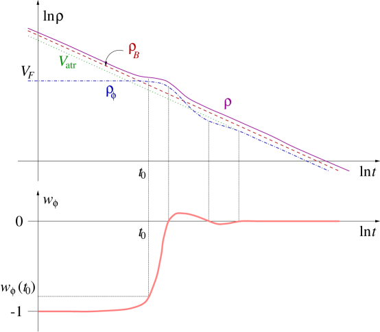
Figure 3: Diagram illustrating the behaviour of the energy density $\rho_{\phi}$ of the scalar field as well as the equation of state parameter $w_{\phi}$ at the moment of unfreezing in the case of the exponential attractor, when coincidence is fixed near this moment. The upper graph shows the evolution of $\rho_{\phi}$ (dot-dash line) and of the background density $\rho_{B}$ (dashed line) near their cross-section point (it may be considered as a close-up of Fig. 2(c) ). When $\rho_{\phi}$ meets the attractor solution $V_{\rm atr}$ (dotted line) it does not immediately unfreeze. Instead it remains “superfrozen” for a brief period, during which it dominates $\rho_{B}$ and results in a “bump” in the down-slope of the decreasing overall energy density $\rho$ (solid line). Then it oscillates briefly around the attractor before settling down to follow it. The above “bump” results in brief acceleration of the Universe expansion, which is necessary to explain the current observations, while avoiding eternal acceleration. During this transition a corresponding change of $w_{\phi}$ from -1 to 0 occurs, as shown in the lower graph. During the brief oscillation period of the system around the attractor, $w_{\phi}$ oscillates around zero. However, during the “bump” in $\rho$ the value of $w_{\phi}$ is still close to -1 because $\rho_{\phi}$, being “superfrozen”, remains almost flat.

It has been shown by numerical simulations that when the scalar field unfreezes and begins to follow the attractor, its trajectory in phase space, just after the transition, oscillates briefly around the attractor evolution path (see Copeland et al. in [16]). This fact, in the case of the exponential tail and when the attractor is really close to dominating the Universe energy density (as suggested by (54) ), enables the field to achieve some acceleration for a limited time interval until it settles to the attractor (see Fig. 3). Thus, attractor quintessence with exponential tail can result in brief but not eternal acceleration [31].

3.1.4 The choice of quintessential tail

String theory considerations disfavor a Universe with eternal acceleration because such a Universe features a future event horizon, which renders the $S$-matrix construction problematic because the asymptotic states of observables are not well defined [33], similarly to the case of de-Sitter space [34]. Moreover, since the de-Sitter vacuum has finite temperature, a system cannot relax into a zero-energy supersymmetric vacuum while accelerating if the evolution is dominated by a single scalar field with a stable potential. If we take this constraint into consideration on our quintessence models then all of frozen quintessence, as well as mild-slope attractor schemes (Figs. 2(a) and 2(d) ) become ruled out. Thus, since steep-slope quintessential tails (Fig. 2(b) ) have disastrous attractors, we conclude that only attractor quintessence with an exponential-tail is admissible for quintessential evolution. Moreover, if we want to achieve brief acceleration we must consider the unfreezing of the field near the present time. Therefore, the best choice seems to be considering $\phi_{0}\simeq\phi_{F}$ and also implementing the attractor constraint (54).

Thus, in search of a model that communicates information from the inflationary era down to the quintessential tail (i.e. a model without phase transitions or a multi-branch potential), we are led to try a quintessential tail of the form,

$$V(\phi\gg\phi_{\rm end})\simeq V_{\rm end}\exp(-\lambda\phi/m_{P})$$ (55)

where $\lambda>0$ is a parameter. Using (11) we obtain $\varepsilon=-\lambda/\sqrt{6}$. Hence, in view of (54) we find for $\lambda$,

$$\lambda\mbox{\raisebox{-3.87495pt}{~{}$\stackrel{{\scriptstyle\mbox{$>$}}}{{\sim}}$~{}}}\sqrt{3/2}$$ (56)

meaning that $\lambda$ should be close but not smaller than $\sqrt{3/2}$. Using this we may employ the coincidence requirement (39), using (33) for $\phi_{0}=\phi_{F}$, to find the corresponding value for $V_{\rm end}$. However, if one does that then it can be shown that, in this case, it is impossible to satisfy the BBN constraint (29). This is because the slope of the exponential tail when $\lambda$ is given by (56) is not sufficient to achieve coincidence and simultaneously retain a high value of $V_{\rm end}$, which would have enabled kination to terminate before the onset of BBN.

Fortunately, there is a way out from this disappointing result. What one may do is attempt to modify the quintessential tail in such a way that the attractor may be preserved, more or less intact but the magnitude of the potential energy density of the scalar field become nevertheless additionally suppressed, compared to the pure exponential tail. This is possible to achieve if one combines the exponential tail with another tail of milder slope. The obvious candidate is the Inverse Power-Law (IPL) tail, which is rather popular in quintessence models and may even have some theoretical motivation [15]. Thus, the suggested quintessential tail is of the form,

$$V(\phi\gg\phi_{\rm end})\simeq V_{\rm end}\frac{\exp(-\lambda\phi/m_{P})}{(\phi/m)^{k}}$$ (57)

where $k\geq 1$ is an integer and $m<m_{P}$ is a mass-scale characteristic of the IPL-slope. The above quasi-exponential quintessential tail has the same attractor solution with the pure exponential one for large values of $\phi$. Indeed, from (33) we see that $\phi_{F}\gg m_{P}$, which suggests,

$$V^{\prime}(\phi_{F})=-\frac{V}{m_{P}}\Big{[}\lambda+k\Big{(}\frac{m_{P}}{\phi_{F}}\Big{)}\Big{]}\simeq-\frac{\lambda V}{m_{P}}$$ (58)

i.e. $V^{\prime}$ approaches the value of the pure exponential tail (corresponding to $k=0$). Thus, since the form of the attractor solution (37) is decided by $V^{\prime}$ and not by $V$, we find that the exponential-tail attractor is attained while there is an additional suppression of the potential energy due to the contribution of the IPL factor.

It is evident that, given a large enough $V_{\rm end}$ (to satisfy the BBN constraint), coincidence is attained with low values of $k$ only when using adequately low values for $m$.

3.2 Insights for the inflationary era

It is easy to see that the exponential behaviour of the potential at the quintessential tail cannot carry over to the inflationary era because of the steepness it results to. Indeed, suppose that the IPL contribution is somehow eliminated at the inflationary part of the potential so that during inflation $V(\phi)$ is given by (55). Then in view of (56) and using (11) we find , $\eta\mbox{\raisebox{-3.87495pt}{~{}$\stackrel{{\scriptstyle\mbox{$>$}}}{{\sim}}$~{}}}1$ i.e. the second slow–roll condition cannot be satisfied and it is impossible to achieve inflation. Obviously any IPL contribution would only make matters worse. Thus, both the exponential and the IPL features have to be modified during the inflationary era. This modification is not trivial.

The prime obstacle is the huge difference between the energy scales of the inflationary plateau and the quintessential tail, $V_{\rm end}\gg V_{F}\sim\rho_{0}$ as required by BBN and coincidence. Given that BBN requires, roughly, that $V_{\rm end}\mbox{\raisebox{-3.87495pt}{~{}$\stackrel{{\scriptstyle\mbox{$>$}}}{{\sim}}$~{}}}10^{13}$GeV, a steep inflationary plateau results either in very brief inflation, which cannot account for the horizon and flatness problems, or, if not taken to be brief, in strongly super-Planckian inflationary energy scale. A flat inflationary plateau, however, because it has to “prepare” for the deep dive towards $V_{F}$ after the end of inflation, typically features a large value of $|V^{\prime\prime}|$, which, through $\eta$, results in unacceptably large values of the spectral index $n$ [c.f. (19)]. Thus, it is not at all easy to design a successful potential for quintessential inflation, let alone using few mass scales and parameters. Nevertheless, it is not impossible as we show in the following example.

4 A Concrete Example

Following the insights given in Sec. 3 we now present a concrete model realization in terms of a specific form of the scalar potential and demonstrate how it meets all the necessary requirements which have been outlined in Sec. 2.

4.1 The model

Consider the potential,

$$V(\phi)=M^{4}[1-\tanh(\phi/m_{P})]\Big{[}1-\sin\Big{(}\frac{\pi\phi/2}{\sqrt{\phi^{2}+m^{2}}}\Big{)}\Big{]}^{k}$$ (59)

where the scalar field $\phi$ lies in the range $-\infty<\phi<+\infty$, $M,\>m<m_{P}$ are two mass parameters and $k>0$ is an integer. This is schematically illustrated in Fig. 4. The above may be written in terms of the dimensionless field variable

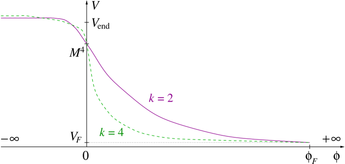
Figure 4: Artist’s view of the potential (59) for $k=2,4$ (solid line and dashed lines respectively). The decrease between the inflationary plateau and the quintessential tail corresponds to a drastic reduction of the energy density by more than a hundred orders of magnitude. However, the differences on the inflationary energy scale, which depend on $k$ are only a few factors of 2. All the models of the family cross at the value $V(\phi=0)=M^{4}$ and $V_{F}=V(\phi_{F})$.

$$x\equiv\frac{\phi}{m}$$ (60)

as follows,

$$V(x)=M^{4}[1-\tanh(zx)]\Big{[}1-\sin\Big{(}\frac{\pi x/2}{\sqrt{1+x^{2}}}\Big{)}\Big{]}^{k}$$ (61)

where

$$z\equiv\frac{m}{m_{P}}$$ (62)

Typically, $0<z\ll 1$. For negative values of $x$ the above becomes,

$$V(x\ll 0)\simeq 2^{k+1}M^{4}(1-e^{2zx}-\frac{k\pi^{2}}{64x^{4}})\simeq 2^{k+1}M^{4}$$ (63)

i.e. it approaches a constant, non-zero, false vacuum energy density which is responsible for driving the inflationary era. On the other hand, for very large positive values of $x$ the potential (61) becomes,

$$V(x\gg 0)\simeq 2^{1-k}(\frac{\pi}{4})^{2k}e^{-2zx}\frac{M^{4}}{x^{4k}}$$ (64)

which has the desired form of the quasi-exponential tail appropriate for quintessence. Note that, in view of (62) and comparing the above with (57) we see that $\lambda=2$, a value which is in good agreement with (56). From (61) we find,

$$V^{\prime}=-\frac{V}{m}\,W\hskip 11.38092pt\mbox{where}\hskip 11.38092ptW(x)\equiv\frac{2z}{1+e^{-2zx}}+\frac{k\pi}{2}\tan\Big{[}\frac{\pi}{4}\Big{(}1+\frac{x}{\sqrt{1+x^{2}}}\Big{)}\Big{]}(1+x^{2})^{-3/2}$$ (65)

and also,

$$V^{\prime\prime} = \frac{V}{m^{2}}\,\left(W^{2}-\frac{dW}{dx}\right)\hskip 56.9055pt\mbox{where}$$ (66)

$$\frac{dW}{dx} = \frac{z^{2}}{[\cosh(zx)]^{2}}+\frac{2k(\pi/4)^{2}}{(1+x^{2})^{3}}\left\{\cos\Big{[}\frac{\pi}{4}\Big{(}1+\frac{x}{\sqrt{1+x^{2}}}\Big{)}\Big{]}\right\}^{-2}-\frac{3k\pi x}{2(1+x^{2})^{5/2}}\tan\Big{[}\frac{\pi}{4}\Big{(}1+\frac{x}{\sqrt{1+x^{2}}}\Big{)}\Big{]}$$

4.2 Inflation

Inflation corresponds to $\phi\ll 0$ or, equivalently, $x\ll 0$. From (11), (65) and (66) we find that, in this region

$$\varepsilon(x\ll 0) \simeq -\frac{1}{\sqrt{6}}\Big{(}\frac{m_{P}}{m}\Big{)}\Big{(}2ze^{2zx}-\frac{k\pi^{2}}{16x^{5}}\Big{)}$$

$$\eta(x\ll 0) \simeq -\frac{1}{3}\Big{(}\frac{m_{P}}{m}\Big{)}^{2}\Big{(}4z^{2}e^{2zx}+\frac{5k\pi^{2}}{16x^{6}}\Big{)}$$

It can be checked that, in the above, the exponential term is dominant in the inflationary region. In view of this fact one finds that inflation is terminated when the second slow-roll condition is violated, i.e. $|\eta(x_{\rm end})|=1$, where $x_{\rm end}\equiv\phi_{\rm end}/m$. Hence, we find,

$$\phi_{\rm end}\simeq-\ln(2/\sqrt{3})\,m_{P}$$ (68)

Thus, we see that $\phi_{\rm end}$ is independent of the mass scales and of $k$.

Inserting the above into (63) we obtain,

$$V_{\rm end}\simeq 2^{k-1}M^{4}$$ (69)

Now, using (14), we find,

$$\phi_{N}\equiv\phi(N)=-\frac{1}{2}\ln[4(N+1/3)]\,m_{P}$$ (70)

which is again independent of $M,m$ and $k$.

Using the above (16) and (17) provide the COBE constraint,

$$\frac{2^{\frac{k+1}{2}}}{\sqrt{3}\,\pi}\Big{(}\frac{M}{m_{P}}\Big{)}^{2}(N_{\rm dec}+1/3)=10^{-5}$$ (71)

This constraint determines the magnitude of the inflationary energy scale $M$ in terms of $k$ and of the reheating efficiency factor $\alpha$. Using (15) and taking $\alpha\simeq 1/100$ and $k\leq 4$ we find,

$$M\sim 10^{15}\>\mbox{GeV}$$ (72)

which is roughly the scale of grand unification similarly to the cases of Chaotic, Hybrid and Natural inflation.

Let us also calculate the spectral index of the density perturbation spectrum. Using (19), (LABEL:neweps) and (70) we find,

$$n(N)-1\simeq-\frac{6}{3N+1}\Big{[}1+\frac{9}{8(3N+1)}\Big{]}$$ (73)

which is independent of $k$ and of the inflationary energy scale $M$. With $\alpha\simeq 1/100$ and using (26) the above gives,

$$n(N_{\rm dec})\approx n(N_{\rm eq})\simeq 0.97$$ (74)

which is in excellent agreement with observations [3].

Using (12), (25), (69) and (71) one finds,

$$T_{\rm reh}\simeq\frac{\alpha}{4}\frac{10^{-5}m_{P}}{\sqrt{N_{\rm dec}+1/3}}\sim 10^{9}\>\mbox{GeV}$$ (75)

which actually saturates the gravitino bound. Finally, from (28), (69) and (71), while also using $g_{*}=106.75$, one obtains,

$$T_{*}\simeq\frac{\alpha^{3}\pi^{2}}{96}\sqrt{\frac{g_{*}}{30}}\frac{10^{-10}m_{P}}{(N_{\rm dec}+1/3)^{2}}\sim 10\;\mbox{MeV}>T_{\rm\sc bbn}$$ (76)

i.e. the BBN constraint is satisfied. Note that the above estimates of $T_{\rm reh}$ and $T_{*}$ are $k$-independent.

Finally, evaluating (22) and (26) one finds that $N_{F}\simeq 57$ and $N_{H}\simeq 74$ respectively, which, using (70), suggests that the horizon and flatness problems are solved if the initial value of the field is,

$$\phi_{\rm in}<-\frac{1}{2}\ln[4(N_{H}+1/3)]\,m_{P}\simeq-2.85\,m_{P}$$ (77)

which is natural to satisfy if one considers that we expect $|\phi_{\rm in}|\sim M_{P}$. Thus, no fine-tuning of initial conditions for inflation is required.

4.3 Quintessence

The quintessential region of the potential (61) corresponds to $\phi\gg 0$. According to (64) the quintessential tail is,

$$V(\phi\gg 0)\simeq 2^{1-k}(\frac{\pi}{4})^{2k}e^{-2\phi/m_{P}}M^{4}\Big{(}\frac{m}{\phi}\Big{)}^{4k}$$ (78)

Let us find the attractor first. Using (35) we find,

$$f(\omega)=\frac{2^{k-3}m^{2}}{\pi^{2k}z^{2(2k+1)}M^{4}}\times I(\omega)\hskip 28.45274pt\mbox{with}\hskip 28.45274pt\omega\equiv 2\phi/m_{P}$$ (79)

where

$$I(\omega)\equiv\int^{\prime}\frac{e^{\omega}\omega^{4k}d\omega}{1+\frac{4k}{\omega}}\simeq e^{\omega}\omega^{4k}\hskip 28.45274pt\mbox{when}\hskip 28.45274pt\omega>4k$$ (80)

In this case we may use (5) and (52) to obtain the attractor solution,

$$V_{\rm atr}(t)=\frac{1}{2}\Big{(}\frac{1-w_{B}}{1+w_{B}}\Big{)}\Big{(}\frac{m_{P}}{t}\Big{)}^{2}\propto t^{-2}$$ (81)

Thus, in view of (5) and (62) we obtain,

$$\frac{V_{\rm atr}}{\rho_{B}}=\frac{3}{8}\,(1-w_{B}^{2})\hskip 28.45274pt\mbox{for}\hskip 28.45274pt\phi_{\rm atr}(t)>2k\,m_{P}$$ (82)

which is in agreement with (54).

As explained in Sec. 3.1.4, in order to achieve a brief period of acceleration (to account for the SN Ia observations) but not eternal acceleration (disfavored by string theory considerations) we need to have attractor quintessence beginning today, i.e. $\phi_{\rm atr}(t_{0})=\phi_{F}$. In this case, since $w_{B}(t_{0})=w_{m}=0$, we have,

$$V_{F}=V_{\rm atr}(t_{0})=\frac{3}{8}\rho_{B}(t_{0})=\frac{3}{11}\,\rho_{0}$$ (83)

where $\rho_{0}=\rho_{B}(t_{0})+V_{F}$. Hence, we see that, because $\Omega_{\phi}\approx 2/3$ coincidence, as defined in (39), is not quite attained when the attractor is met. Indeed, for coincidence we need $V_{F}=2\rho_{B}(t_{0})$. However, if this were so, because $V_{\rm atr}(t_{0})=V_{F}$ we would have had eternal acceleration, according to (53). Still, coincidence may be attained briefly because of the oscillations of the scalar field evolutionary track around the attractor (81), just after the unfreezing of the field. These oscillations are due to the fact that the field retains its frozen value for a little while after crossing over the attractor’s path, being effectively “superfrozen”. This may increase somewhat the ratio $V_{F}/\rho_{0}$ before the field actually unfreezes. Since we only require an increase of the order of $\sim\frac{\Delta\Omega_{\phi}}{\Omega_{\phi}}\approx 3/5$, we feel that coincidence is realistically possible to achieve. Moreover, while the field is “superfrozen” we expect that $w_{\phi}\approx-1$. However, in order to obtain a specific value of $w_{\phi}$ numerical simulations are necessary. Still, we are confident that successful coincidence can be attained by minute adjustments of the mass scales, which suggests that our treatment is sufficient for order of magnitude estimates of $m,M$ (see also Sec. 5).

In the following we will use (83) to estimate the mass-scale $m$. The frozen value of the field is estimated by (33), (68) and (69) to be,

$$\phi_{F}=\sqrt{6}\left\{\frac{2}{3}-\frac{1}{\sqrt{6}}\ln(2/\sqrt{3})+\ln\left[\frac{24}{\alpha^{2}}\sqrt{\frac{10}{g_{*}}}(N_{\rm dec}+1/3)10^{5}\right]\right\}m_{P}$$ (84)

where we have also used (71). Note that $\phi_{F}$ is independent of the mass scales $M,m$ and of $k$, similarly to $\phi_{\rm end}$. For $\alpha\simeq 1/100$ and $g_{*}=106.75$ the above suggests that $\phi_{F}\simeq 67\,m_{P}$, i.e. $\phi_{F}/m_{P}>4k$  for $k\leq 4$ and we are, therefore, safely into the region of the exponential attractor, as previously assumed in (80).

Inserting (84) into (64) and employing (83), after a little algebra we find,

$$m = 4\sqrt{3\pi}\left\{\frac{2}{3}-\frac{1}{\sqrt{6}}\ln(2/\sqrt{3})+\ln\left[\frac{24}{\alpha^{2}}\sqrt{\frac{10}{g_{*}}}(N_{\rm dec}+1/3)10^{5}\right]\right\}\;\times$$

$$\times \left\{\frac{3}{44\pi^{2}}(N_{\rm dec}+1/3)^{2}10^{10}\left[\frac{24e^{2/3}}{\alpha^{2}}\sqrt{\frac{10}{g_{*}}}(N_{\rm dec}+1/3)10^{5}\right]^{2\sqrt{6}}\right\}^{1/4k}\Big{(}\frac{\rho_{0}^{1/4}}{m_{P}}\Big{)}^{1/k}m_{P}$$

where we used (62) and (71). With $\alpha\simeq 1/100$ and $g_{*}=106.75$ the above becomes,

$$m\sim 4\times 10^{2}(3\times 10^{70})^{1/4k}10^{-30/k}\,m_{P}$$ (86)

Thus, we see that the highest the value of $k$ the largest the magnitude of $m$. This is easily understood as follows. Since $k$ determines the IPL decrease of the potential energy $V$ of the scalar field in the quintessential part of its evolution, a large $k$ results in substantial suppression of $V$. This allows $m$, to which $V$ is proportional [c.f. (78)], to be large. In the opposite case, however, the decrease of $V$ is not as substantial. As a result $m$ has to be small so that $V$ may manage to drop as low as $\rho_{0}$.

In the next table we show the values of $m$ for small values of $k$.

$k$	1	2	3	4
$m$	$10^{8}$ GeV	$10^{15}$ GeV	$10^{17}$ GeV	$10^{18}$ GeV

From this table it is clear that we should consider only $k\leq 4$ in order to avoid super-Planckian values of $m$, which would result by higher values of $k$. Note also that for $m\sim m_{P}$ we have $\phi_{\rm end},\phi_{F}={\cal O}(1)\times m_{P}$ and, therefore, the approximations used to obtain (63) and (64) are challenged. Still, we believe that even in this case our treatment remains valid for order-of-magnitude estimates, especially for quantities like $T_{*},T_{\rm reh},n$ or even $M$, which are essentially independent of $k$. From the above table we notice also that for $k=2$ we may identify $m=M$. Similarly, for $k=4$ we may consider $m=m_{P}$. Thus, in these cases we attain successful quintessential inflation with the use of only two, natural mass scales, the Planck mass and the scale of grand unification. These two models are:

• Model 1:

  $$V(\phi)=M^{4}[1-\tanh(\phi/m_{P})]\Big{[}1-\sin\Big{(}\frac{\pi\phi/2}{\sqrt{\phi^{2}+M^{2}}}\Big{)}\Big{]}^{2}$$ (87)

• Model 2:

  $$V(\phi) = M^{4}(\phi)\;[1-\tanh(\phi/m_{P})]$$

  $$M(\phi) \equiv M\Big{[}1-\sin\Big{(}\frac{\pi\phi/2}{\sqrt{\phi^{2}+m_{P}^{2}}}\Big{)}\Big{]}$$

Both these models provide inflation at the scale of grand unification, with reheating temperature $T_{\rm reh}\sim 10^{9}$GeV and spectral index of the density perturbation spectrum $n\simeq 0.97$. Also, since the field unfreezes at the present time we expect a brief period of acceleration with $w_{\phi}\approx-1$.

However, to obtain a precise value of $w_{\phi}$ one would have to employ numerical simulations. In the first of [31] such numerical simulations suggest that successful coincidence may be achieved with $\lambda\approx 3/2$. We can obtain this in our model if we take $m_{P}\rightarrow\frac{4}{3}\,m_{P}$ in (59). The subsequent results are largely unaffected, except the value of $m$ which is reduced, as expected. It turns out that, in this case, one can have $m\sim M\sim 10^{15}$GeV for $k=4$. Thus, according to those numerical simulations, another successful quintessential inflationary model would be,

$\bullet$ Model 3:

$$\begin{array}[]{lll}V(\phi)&=&M^{4}(\phi)\;[1-\tanh(\frac{3}{4}\phi/m_{P})]\\ &&\\ M(\phi)&\equiv&M\Big{[}1-\sin\Big{(}\mbox{\large$\frac{\pi\phi/2}{\sqrt{\phi^{2}+M^{2}}}$}\Big{)}\Big{]}\end{array}$$ (89)

Note that Model 1 of the above models may be constructed in the context of the theoretical framework of [24] by considering the pre-potentials, $V_{1}(\phi)\equiv M^{4}\sin\Big{(}$$\frac{\pi\phi/2}{\sqrt{\phi^{2}+M^{2}}}$$\Big{)}$ and $V_{2}(\phi)\equiv\frac{1}{4}M^{4}/[1-\tanh(\phi/m_{P})]=\frac{1}{8}M^{4}(e^{2\phi/m_{P}}+1)$.

5 Discussion and conclusions

We have developed general criteria required in unified frameworks for inflation and quintessence in which a single scalar field is chosen to drive both. By using such a minimal field content we avoid having to fine-tune couplings and mass-scales. Moreover, the initial conditions for quintessence are fixed at the end of the inflationary epoch.

Quintessential inflation is realized if the scalar potential features two flat regions, the inflationary plateau and the quintessential tail. Inflation in such models is of the non-oscillatory type, in which reheating is achieved due to the gravitational production of particles at the end of the inflationary period. Such reheating is inefficient and leads to a brief period of kination, which has to be terminated before Big Bang Nucleosynthesis. After kination the Universe evolves according to the Standard Hot Big Bang, while the scalar field lies frozen until the present epoch, when, once more, its potential energy density becomes comparable with the background density of the Universe, leading to the currently observed accelerated expansion.

Our treatment suggests that, in order to achieve a brief acceleration period occurring at present the quintessential tail of the scalar potential should be of quasi-exponential form. Also, the inflationary plateau should be such that the deep drop towards the quintessential tail does not result in an excessive value for the spectral index of density perturbations and CMBR anisotropies. We have demonstrated that the above are, indeed, possible to achieve and have presented and analyzed a class of successful models. In our quintessential inflationary models the inflationary energy scale is of the order of the scale of grand unification, similarly to Hybrid, Chaotic and Natural inflation. The reheating temperature, however, is low enough not to violate the gravitino constraint. Moreover, inflation manages to satisfy the COBE normalization constraint, to easily account for the horizon and flatness problems and, finally, to result in a CMBR spectral index $n\approx 0.97$, in remarkable agreement with the latest CMBR data. As far as the quintessential part is concerned our models lead to a brief acceleration period by unfreezing the scalar field at present. Because the field is briefly “superfrozen” we expect that $w_{\phi}\approx-1$ as required.

Two of our models are singled out because they achieve the desired results with the use of only two, natural mass scales, namely the Planck mass and the grand unification energy scale. Thus, these models do not introduce any additional fine tunning for quintessence and in that respect they outshine the cosmological constant alternative.

Similar to other models of quintessence, ours also requires the expectation value of the field today to be of order the Planck mass. This fact is an indicator that we may realize our model in the context of supergravity. Indeed, hidden sector fields in supergravity and/or superstring models offer, potentially natural, candidates for our “double-task” scalar field $\phi$. Other alternatives include moduli fields or the radion field in models with large extra dimensions. Seeking for a detailed derivation of the possible forms of the scalar potential from a “Theory of Everything” lies however outside the scope of our present paper, which is mainly phenomenological. Nevertheless, we find it remarkable that such quintessential inflationary potentials, meeting all the required constraints and requirements, are possible to construct with the use of only one scalar field and very few natural mass scales.

Acknowledgments

Work supported by Spanish grant PB98-0693 and by the European Commission RTN network HPRN-CT-2000-00148

References

- [1] S. Perlmutter et al. [Supernova Cosmology Project Collaboration], Astrophys. J. 517 (1999) 565 [astro-ph/9812133]; A. G. Riess et al. [Supernova Search Team Collaboration], Astron. J. 116 (1998) 1009 [astro-ph/9805201]; B. P. Schmidt et al., Supernovae,” Astrophys. J. 507 (1998) 46 [astro-ph/9805200]; P. M. Garnavich et al., Astrophys. J. 493 (1998) L53 [astro-ph/9710123].
- [2] R. G. Carlberg et al., Astrophys. J. 478 (1997) 462 [astro-ph/9703107]; N. Bahcall et al., Science 284 (1999) 1481 [astro-ph/9906463]; M. Tegmark, Astrophys. J. 514 (1999) L69 [astro-ph/9809201].
- [3] P. D. Mauskopf et al., Astrophys. J. 536 (2000) L59 [astro-ph/9911444]; N. W. Halverson et al., [astro-ph/0104489]; C. Pryke, N. W. Halverson, E. M. Leitch, J. Kovac, J. E. Carlstrom, W. L. Holzapfel and M. Dragovan, [astro-ph/010449]; S. Hanany et al., Astrophys. J. 545 (2000) L5 [astro-ph/0005123]; A. Balbi et al., Astrophys. J. 545 (2000) L1 [astro-ph/0005124].
- [4] A. H. Jaffe et al., Phys. Rev. Lett. 86 (2001) 3475 [astro-ph/0007333].
- [5] For a review see S. Weinberg, Rev. Mod. Phys. 61 (1989) 1.
- [6] J. D. Barrow and F. J. Tipler, “The anthropic Cosmological Principle”, Oxford University Press (1986) 668.
- [7] P. J. Peebles and B. Ratra, Astrophys. J. 325 (1988) L17.
- [8] K. Coble, S. Dodelson and J. A. Frieman, Phys. Rev. D 55 (1997) 1851 [astro-ph/9608122]; J. L. Lopez and D. V. Nanopoulos, Mod. Phys. Lett. A 11 (1996) 1 [hep-ph/9501293]; A. D. Linde, Phys. Lett. B 351 (1995) 99 [hep-th/9503097]; N. Weiss, Phys. Lett. B 197 (1987) 42.
- [9] L. Wang, R. R. Caldwell, J. P. Ostriker and P. J. Steinhardt, Astrophys. J. 530 (2000) 17 [astro-ph/9901388]; I. Zlatev, L. Wang and P. J. Steinhardt, Phys. Rev. Lett. 82 (1999) 896 [astro-ph/9807002]; G. Huey, L. M. Wang, R. Dave, R. R. Caldwell and P. J. Steinhardt, Phys. Rev. D 59 (1999) 063005 [astro-ph/9804285]; R. R. Caldwell, R. Dave and P. J. Steinhardt, Phys. Rev. Lett. 80 (1998) 1582 [astro-ph/9708069].
- [10] T. Matos and L. A. Urena-Lopez, Class. Quant. Grav. 17 (2000) L75 [astro-ph/0004332]; A. de la Macorra and G. Piccinelli, Phys. Rev. D 61 (2000) 123503 [hep-ph/9909459]; P. F. Gonzalez-Diaz, Phys. Rev. D 62 (2000) 023513 [astro-ph/0004125]; S. M. Carroll, Phys. Rev. Lett. 81 (1998) 3067 [astro-ph/9806099].
- [11] P. J. Steinhardt, L. Wang and I. Zlatev, Phys. Rev. D 59 (1999) 123504 [astro-ph/9812313]; S. C. Ng, N. J. Nunes and F. Rosati, Phys. Rev. D 64 (2001) 083510 [astro-ph/0107321]; V. B. Johri, Phys. Rev. D 63 (2001) 103504 [astro-ph/0005608].
- [12] K. Choi, Phys. Rev. D 62 (2000) 043509 [hep-ph/9902292]. M. C. Bento and O. Bertolami, Gen. Rel. Grav. 31 (1999) 1461 [gr-qc/9905075]. R. Bean and J. Magueijo, Phys. Lett. B 517 (2001) 177 [astro-ph/0007199].
- [13] L. Amendola, Mon. Not. Roy. Astron. Soc. 312 (2000) 521 [astro-ph/9906073]. F. Perrotta, C. Baccigalupi and S. Matarrese, Phys. Rev. D 61 (2000) 023507 [astro-ph/9906066]; Y. Fujii, Phys. Rev. D 62 (2000) 044011 [gr-qc/9911064]; N. Bartolo and M. Pietroni, Phys. Rev. D 61 (2000) 023518 [hep-ph/9908521]; O. Bertolami and P. J. Martins, Phys. Rev. D 61 (2000) 064007 [gr-qc/9910056]; T. Chiba, Phys. Rev. D 60 (1999) 083508 [gr-qc/9903094].
- [14] A. Albrecht, C. P. Burgess, F. Ravndal and C. Skordis, [astro-ph/0107573]; S. H. Tye and I. Wasserman, Phys. Rev. Lett. 86 (2001) 1682 [hep-th/0006068]; P. F. Gonzalez-Diaz, Phys. Lett. B 481 (2000) 353 [hep-th/0002033]; C. P. Burgess, R. C. Myers and F. Quevedo, Phys. Lett. B 495 (2000) 384 [hep-th/9911164]; N. Arkani-Hamed, S. Dimopoulos, N. Kaloper and R. Sundrum, Phys. Lett. B 480 (2000) 193 [hep-th/0001197]; J. M. Cline, C. Grojean and G. Servant, Phys. Rev. Lett. 83 (1999) 4245 [hep-ph/9906523]; V. A. Rubakov and M. E. Shaposhnikov, Phys. Lett. B 125 (1983) 139.
- [15] E. J. Copeland, N. J. Nunes and F. Rosati, Phys. Rev. D 62 (2000) 123503 [hep-ph/0005222]; P. Brax and J. Martin, Phys. Lett. B 468 (1999) 40 (1999) [astro-ph/9905040]; Annalen Phys. 11 (2000) 507 [astro-ph/9912005]; A. Masiero, M. Pietroni and F. Rosati, Phys. Rev. D 61 (2000) 023504 [hep-ph/9905346]; P. Binetruy, Phys. Rev. D 60 (1999) 063502 [hep-ph/9810553].
- [16] T. Barreiro, E. J. Copeland and N. J. Nunes, Phys. Rev. D 61 (2000) 127301 [astro-ph/9910214]; E. J. Copeland, A. R. Liddle and D. Wands, Phys. Rev. D 57 (1998) 4686 [gr-qc/9711068]; P. G. Ferreira and M. Joyce, Phys. Rev. D 58 (1998) 023503 [astro-ph/9711102]; Phys. Rev. Lett. 79 (1997) 4740 [astro-ph/9707286].
- [17] C. Kolda and D. H. Lyth, Phys. Lett. B 458 (1999) 197 [hep-ph/9811375].
- [18] A. Albrecht and P. J. Steinhardt, Phys. Rev. Lett. 48 (1982) 1220.
- [19] P. de Bernardis et al., Nature 404, 955 (2000) [astro-ph/0004404].
- [20] For a review see D. H. Lyth and A. Riotto, Phys. Rept. 314 (1999) 1 [hep-ph/9807278] and references therein.
- [21] R. A. Frewin, J. E. Lidsey, Int. J. Mod. Phys. D 2 (1993) 323
- [22] P. J. Peebles and A. Vilenkin, Phys. Rev. D 59 (1999) 063505 [astro-ph/9810509]; see also C. Baccigalupi and F. Perrotta, [astro-ph/9811385]; M. Giovannini, Class. Quant. Grav. 16 (1999) 2905 [hep-ph/9903263].
- [23] W. H. Kinney and A. Riotto, Astropart. Phys. 10 (1999) 387 [hep-ph/9704388]; M. Peloso and F. Rosati, JHEP 9912 (1999) 026 [hep-ph/9908271].
- [24] A. B. Kaganovich, Phys. Rev. D 63 (2001) 025022 [hep-th/0007144].
- [25] G. Huey and J. E. Lidsey, Phys. Lett. B 514 (2001) 217 [astro-ph/0104006]; A. S. Majumdar, Phys. Rev. D 64 (2001) 083503 [astro-ph/0105518].
- [26] G. N. Felder, L. Kofman and A. D. Linde, Phys. Rev. D 60 (1999) 103505 [hep-ph/9903350].
- [27] L. H. Ford, Phys. Rev. D 35 (1987) 2955.
- [28] M. Joyce and T. Prokopec, Phys. Rev. D 57 (1998) 6022 [hep-ph/9709320].
- [29] B. Spokoiny, Phys. Lett. B 315 (1993) 40 [gr-qc/9306008].
- [30] K. Dimopoulos, Proceedings of the EURESCO Conference on Frontiers in Particle Astrophysics and Cosmology, San Feliu de Guixols, Spain, edited by M. Hirsch, G. Raffelt, J. W. F. Valle, ISSN 0920-5632, Nucl. Phys. Proc. Suppl. 95 (2001) 70 [astro-ph/0012298].
- [31] J. M. Cline, JHEP 0108 (2001) 035 [hep-ph/0105251]. C. Kolda and W. Lahneman, [hep-ph/0105300].
- [32] M. Li, W. Lin, X. Zhang and R. H. Brandenberger, [hep-ph/0107160].
- [33] S. Hellerman, N. Kaloper and L. Susskind, JHEP 0106 (2001) 003 [hep-th/0104180]; W. Fischler, A. Kashani-Poor, R. McNees and S. Paban, JHEP 0107 (2001) 003 [hep-th/0104181].
- [34] E. Witten, [hep-th/0106109].
- [35] E. Halyo, [hep-ph/0105216]; J. A. Gu and W. Y. Hwang, [astro-ph/0106387]; X. G. He, [astro-ph/0105005]; M. C. Bento, O. Bertolami and N. C. Santos, [astro-ph/0106405].