Temperature Isotropization in Solar Flare Plasmas due to the Electron Firehose Instability

The isotropization process of a collisionless plasma with an electron temperature anisotropy along an external magnetic field ($T_{\|}^{e}\gg T_{\perp}^{e}$, $\|$ and $\perp$ with respect to the background magnetic field) and isotropic protons is investigated using a particle-in-cell (PIC) code. Restricting wave growth mainly parallel to the external magnetic field, the isotropization mechanism is identified to be the Electron Firehose Instability (EFI). The free energy in the electrons is first transformed into left-hand circularly polarized transverse low-frequency waves by a non-resonant interaction. Fast electrons can then be scattered towards higher perpendicular velocities by gyroresonance, leading finally to a complete isotropization of the velocity distribution. During this phase of the instability, Langmuir waves are generated which may lead to the emission of radio waves. A large fraction of the protons is resonant with the left-hand polarized electromagnetic waves, creating a proton temperature anisotropy $T_{\|}^{p}<T_{\perp}^{p}$. The parameters of the simulated plasma are chosen compatible to solar flare conditions. The results indicate the significance of this mechanism in the particle acceleration context: The EFI limits the anisotropy of the electron velocity distribution, and thus provides the necessary condition for further acceleration. It enhances the pitch-angle of the electrons and heats the ions.

1 Introduction

The energization of large numbers of particles to high energies is still an unsolved problem in solar flare research. The vast diversity of observational data imposes severe constraints, for which any acceleration model has to account. The current models can broadly be assigned to three different categories: Shock acceleration, acceleration by parallel electrical fields and stochastic acceleration by cascading MHD waves. For a review of these mechanisms, see e.g. Miller et al (1997).

One restriction on the acceleration model is imposed by the time scales at which the process has to operate: Hard X-ray observations revealed spiky structures as short as $\approx 400$ ms (Kiplinger et al, 1984; Machado et al, 1993). Assuming a thick-target emission process for the radiation, the electrons have to be accelerated to energies above $20$ keV within the given time in each of these spikes. It is believed that these ‘energy release fragments’ are the basic constituent of the entire impulsive phase (Machado et al, 1993). Further fragmentation of the energy release and electron acceleration process was proposed based on decimetric radio emission (Benz, 1985), with temporal structures well below $\approx 10$ ms.

Assuming an isotropic electron velocity distribution, Miller et al (1996) showed that stochastic acceleration can account for energization of electrons from thermal energies up and above $20$keV in less than $400$ ms. However, the actual particle acceleration mechanism in this model, Transit-Time Damping (Fisk, 1976; Stix, 1992), increases only the velocity component parallel to the external magnetic field. In absence of an additional pitch-angle scattering mechanism, this would lead to an anisotropic electron velocity distribution, reducing the efficiency of the acceleration mechanism. Due to the low density and the high temperature, the mean free path between Coulomb collisions in a solar flare plasma is large. The scattering mechanism has therefore to be of a different nature, presumably a wave-particle interaction.

Predominant acceleration along an external magnetic field $B_{0}$ compared to the acceleration in perpendicular direction is not only a problem of Transit-Time damping, but common to all the aforementioned acceleration mechanisms. The isotropization in case of particle acceleration by a sub-Dreicer DC field has been investigated by Moghaddam-Taaheri and Goertz (1990). Assuming quasi-linear diffusion and a wave spectrum due to the runaway electrons (Gandy et al, 1983), they found that the actual isotropization mechanism is anomalous Doppler resonance of fast particles and that a bump in the reduced velocity distribution is formed.

In this paper, the isotropization process of an electron temperature anisotropic plasma without further energy input is addressed. The free energy in the anisotropic electron velocity distribution may drive an instability. The instability would lead to wave growth which in turn can scatter the particles in velocity space. One proposed instability for a electron temperature anisotropic plasma is the Electron Firehose Instability (EFI) (Hollweg and Völk, 1970; Paesold and Benz, 1999; Li and Habbal, 2000). It is a kinetic version of the MHD firehose instability (Rosenbluth, 1956; Parker, 1958) with a lower threshold in electron velocity anisotropy. But is this mechanism actually responsible for the isotropization of the electron velocity anisotropy? The previous investigations of this mechanism were based on linear theory, thus stopped before wave growth effects the particle distribution. If the EFI actually grows or if another instability isotropizes the plasma quicker cannot be answered within the framework of linear theory. Also questions about wave growth saturation are beyond reach of linear theory.

Here, the isotropization mechanism of an electron temperature anisotropy is investigated by means of particle-in-cell (PIC) simulations, giving access to the non-linear effects on the particle distribution as well as the saturation of the instability. The parameters for the simulation are chosen to be compatible with parameters expected under solar flare conditions. While rough estimates for density, ambient magnetic field and electron temperature exist (e.g. Miller et al, 1997), values of the actual anisotropy depend on the exact details of the acceleration mechanism. The anisotropy chosen here is $T^{e}_{\|}/T^{e}_{\perp}=20$ in accordance with earlier estimates (Paesold and Benz, 1999). The simulated plasma corresponds to a population of electrons accelerated from $3$keV to $25$keV without any instabilities.

The paper is organized as follows: Section 2 describes the simulation model, followed by a presentation of the overall development of the isotropization process in Sect. 3. The responsible instability is then identified by comparison with linear theory in Sect. 4. Non-linear processes are discussed in Sect. 5, followed by an investigation of the energy flow in Sect. 6. A discussion of the applicability of result onto real plasmas (Sect. 7) and of the relevance of the described mechanism summarizes the results in Sect. 8.

2 Simulation Model

The simulations were performed with the fully 3D relativistic electromagnetic particle-in-cell code par-T (Messmer, 2000), a parallel implementation of TRISTAN (Buneman, 1993). As both particle species are expected to play a role in the electron firehose instability, they both have to be treated kinetically. This prevents the use of hybrid simulations which treat one particle species as a fluid.

A PIC code traces the trajectories of a representative number of particles under the influence of the Newton-Lorentz force in their self-consistent electromagnetic fields. The particles can be placed anywhere within the computational domain, whereas the field quantities are located on a regular spatial grid. Subgrid resolution, e.g. in order to determine the forces at the particle positions, is obtained by linear interpolation. For an introduction on PIC see e.g. Birdsall and Langdon (1985).

Time integration for both particles and fields is performed by a leap-frog scheme. The fields are staggered in space (Yee, 1966), allowing e.g. to update the B-field by computing the curl of the E-field, using finite differences. This method has the advantage of being simple to implement and additionally to keep $\nabla B=0$, if it was satisfied initially. In oder to update the E-field, the current density has to be determined in addition to the curl of B. Instead of solving the Poission equation explicitly, the herein used code applies a charge conserving current deposition algorithm (Villasenor and Buneman, 1992). This scheme allows to update the E-field entirely from information within a few grid cells. Additionally it keeps $\nabla E=\rho$ satisfied, if it was satisfied initially, down to machine accuracy.

The size of the simulation box is $L_{x}\times L_{y}\times L_{z}=8\Delta\times 8\Delta\times 768\Delta$, where $L_{j}$ is the length of the system in dimension $j$, $\Delta=0.13c/\omega_{e}$ represents the cell size, $\omega_{e}$ is the electron plasma frequency and $c$ is the speed of light. Periodic boundary conditions in all three dimensions are applied on both particles and fields. The total particle number is $2\cdot n_{p}=3.17\cdot 10^{6}$ particles, an average of 32 electron-proton pairs per cell. The particles are placed uniformly within the computational domain. The simulation time step is $\omega_{e}\Delta t=2\pi/100$. Along the $z$-axis, the external magnetic field $B_{0}$ is applied, leading to a ratio $\Omega_{e}/\omega_{e}=0.13$, where $\Omega_{e}$ is the electron cyclotron frequency. Assuming a particle density of $n=5\cdot 10^{10}{\rm cm}^{-3}$, the external magnetic field is $B_{0}=91$ Gauss. As the isotropization is expected to take place on proton time scales, an artificial proton/electron-mass ratio $m_{p}/m_{e}=49$ is chosen, a tribute to computing time. The proton plasma frequency is therefore $\omega_{p}/\omega_{e}=0.14$ and the proton cyclotron frequency $\Omega_{p}/\omega_{e}=0.0026$. The initial electric field is $E_{0}=0$ everywhere within the computational domain by placing electrons and protons at the same positions.

Initially, the electron temperature parallel to the external field is $T_{\|}^{e}=2.3\cdot 10^{8}$ K while the perpendicular electron temperature $T_{\perp}^{e}$ is identical to the isotropic proton temperature $T^{p}=1.2\cdot 10^{7}$ K. The electron temperature ratio is therefore $T_{\|}^{e}/T_{\perp}^{e}\approx 20$. The corresponding thermal velocities are for electrons $v_{\|}^{e}/c=0.2$ and $v_{\perp}^{e}/c=0.045$. The Debye lengths are $\lambda_{D,\|}=1.53\Delta$ and $\lambda_{D,\perp}=0.34\Delta$.

By choosing a rod shaped geometry, wave numbers at oblique angles are limited to values $k>k_{\perp}^{\min}=k_{\|}^{\min}L_{z}/L_{x}=42\omega_{p}/c$, where $k_{\|}^{\min}$ is the minimum wave number in parallel direction. The simulation can therefore be considered as a 1D simulation.

The instability is expected to grow on timescales of proton cyclotron periods. This makes it necessary to run the simulation at least for several proton cyclotron periods. On the other hand, the free energy is carried by the electrons, requiring resolution of the electron plasma frequency. Even with an artificially low mass ratio, this leads to several thousand timesteps per inverse proton cyclotron frequency. To overcome the enormous computing effort, a parallelized simulation code was applied. Ideally, such a code requires a computing time $\tau_{p}=\tau/N_{p}$, where $N_{p}$ is the number of processors, as compared to $\tau$, the time required by the sequential code. In a more realistic model, the speedup $S=\tau/\tau_{p}<N_{p}$, mainly due to the overhead introduced by the communication among the processors. However, in case of a particle-in-cell code with charge conserving current update (Villasenor and Buneman, 1992) only local information is used to solve the field equations. Consequently most of the time is spent in pushing particles and updating field quantities, letting communication be of minor influence. The code does therefore not benefit from a highly sophisticated interconnection network. It can easily be run on a cluster of workstations, which are usually much cheaper and more available than commercial parallel computers. The simulations were therefore performed on a Beowulf-Cluster featuring 48 Pentium-III processors. The total simulation time of 120’000 time steps requires 24 hours, including diagnostics. At a lower limit of the parallel efficiency of $\epsilon\approx 0.8$ on $48$ processors (Messmer, 2000), this corresponds to about $920$ hours of the original TRISTAN code on a single Pentium III processor.

3 Overall Development

Figure 1: Temporal development of the local electron temperatures (top) and proton temperatures (bottom), compared to the temperature development in case of an isotropic plasma (thin dash-dotted lines). Temperatures are shown along the three spatial dimensions $x,y,z$ (dotted, dashed, solid).

Figure 1 shows the development of the local temperatures for both the electrons and the protons during the instability. As both the electron and the proton velocity distribution may not stay Maxwellian throughout the instability, a global temperature is not defined. The local temperature is defined as the standard deviation in one velocity component for a set of particles in a small subdomain of the computational domain. The temperature of the distribution is then defined as the average of all local temperatures.

During the simulated time of $18\Omega_{p}^{-1}$, the inital electron temperature ratio reduces to $T_{\|}^{e}/T_{\perp}^{e}\leq 1.2$. The free energy in the electrons goes partially into the waves, but mainly into the perpendicular electron temperature. This will be shown in Sect. 6. Additionally the protons are slightly heated in all directions. At about $8\Omega_{p}^{-1}$, the proton velocity distribution is becoming anisotropic with $T^{p}_{\perp}>T^{p}_{\|}$. The oscillations are an indicator of energy transfer between the protons and the waves.

For comparison, the parallel temperature development of an isotropic plasma is also plotted in Fig. 1. As expected, the temperature does practically not change throughout the simulated time. This is a first indicator of energy conservation within the simulation.

Figure 2: Temporal development of $B_{\perp}^{2}/B_{\|}^{2}$ for the anisotropic electron velocity distribution with $T_{\|}^{e}/T_{\perp}^{e}\approx 20$ (solid) and $T_{\perp}^{e}=T^{p}$, compared to the development of $B_{\perp}^{2}/B_{\|}^{2}$ for an isotropic electron distribution with $T_{\|}^{e}=T_{\perp}^{e}=T^{p}$ (dotted).

Figure 2 shows the time history of the perpendicular magnetic field energy $B_{\perp}^{2}=\int\!\!\!\int\!\!\!\int(B_{x}^{2}+B_{y}^{2})dx\,dy\,dz$. The development of $B_{\perp}^{2}$ for a simulated plasma with isotropic temperatures $T_{\|}^{e}=T_{\perp}^{e}=T^{p}$ but otherwise identical parameters is again included for comparison.

After a slow increase during $8\Omega_{p}^{-1}$, the energy in $B_{\perp}$ increases explosively, saturates at $12.5\Omega_{p}^{-1}$ and then starts to oscillate, indicating the growth of transverse (electro)magnetic waves.

4 Comparison with Linear Theory

Figure 3: Temporal development of $|B_{x}|$ for the wave number $kc/\omega_{p}=1.32$.

In order to investigate the isotropization further, the excited waves have to be identified. The wave numbers are determined by Fourier transform of $B_{x}$, one component of the perpendicular B-field. Figure 3 shows the temporal evolution of the spatial mode $kc/\omega_{p}=1.32$ propagating parallel to $B_{0}$. After an initial phase of $\approx 1\Omega_{p}^{-1}$, a regular oscillation starts with exponentially growing amplitude. Close to $13\Omega_{p}^{-1}$, the wave growth stops and the oscillation continues.

To identify the wave mode responsible for the growing field $B_{\perp}$, the growth rates of different wave numbers are compared to the values obtained by WHAMP (Rönnmark, 1982). This program allows to evaluate the plasma dispersion function numerically for arbitrary temperature ratios.

Figure 4: Growth rate of $B_{x}$ determined from simulations with $m_{p}/m_{e}=49$ (asterisk) and $m_{p}/m_{e}=81$ (boxes) compared to results obtained from linear theory for $m_{p}/m_{e}=[49,81,1836]$ (dotted, dashed, dash-dotted) for the initial electron temperature ratio $T^{e}_{\|}/T^{e}_{\perp}\approx 20$. In addition, the growth rate for $T^{e}_{\|}/T^{e}_{\perp}\approx 6$ and $m_{p}/m_{e}=49$ is shown (dotted, thin).

Figure 4 shows a comparison of the growth rates between linear theory and PIC simulation. The linear theory results are determined for the initial plasma parameters. The growth rates of the PIC simulation are measured by a linear fit in the time series of spatial Fourier transforms of $B_{x}$ in the time interval $2-8\Omega_{p}^{-1}$. The three growing waves and the suppressed growth at $kc/\omega_{p}=1.76$ are well in accordance with linear theory. However, the growth rates for $kc/\omega_{p}=[0.44,0.88]$ are too low, whereas the one for $kc/\omega_{p}=1.32$ is too high. This will be investigated in Sect. 5.1.

In order to check the influence of the artificial mass ratio, the growth rates are determined for an increased mass ratio of $m_{p}/m_{e}=81$ and otherwise identical plasma parameters (see Fig. 4). Due to the larger mass ratio and the fixed simulation box size of $100c/\omega_{e}$, the resolution in wave numbers decreases. Again, the waves grow in accordance with linear theory, but the determined growth rates are lower than expected for $kc/\omega_{p}=0.59$ and a bit larger for $kc/\omega_{p}=1.18$. For comparison, the growth rates for the real mass ratio $m_{p}/m_{e}=1836$ is included in Fig. 4. The hypothetical light weight protons inhibit wave growth at large k.

Figure 5: Comparison of the dispersion relations obtained by the simulation (asterisk) and by WHAMP (dashed). For comparison, the dispersion relation for the real mass ratio $m_{p}/m_{e}=1836$ is included (dash-dotted).

Figure 5 shows a comparison of the dispersion relation determined both by WHAMP and from the simulation. Due to the limited resolution in k-space, only 3 samples lie within the range of non-zero growth (see Fig. 4). According to linear theory, the period of the sample with smallest wave number, $kc/\omega_{p}=0.44$, is $45\Omega_{p}^{-1}$ and thus much longer than the saturation time of the instability. The frequency can therefore not be measured in the simulation and only an upper bound can be given. For the other two samples, the frequencies are determined by removing the exponential growth and measuring the time between the first two amplitude minima, thus the first half period. Like the growth rates, the wave frequencies agree well with the values determined from linear theory. However, they are both too low.

Table 1: Comparison of growth rates $[\gamma_{0.44},\gamma_{0.88},\gamma_{1.32}]$ between simulation (bold) and linear theory at $kc/\omega_{p}=[0.44,0.88,1.32]$ and wave number of maximum growth $k_{m}$ for different electron temperature ratios $T^{e}_{\|}/T^{e}_{\perp}$. The other plasma parameters are identical to Sect. 2.

$T^{e}_{\|}/T^{e}_{\perp}$	$\gamma_{0.44}/\Omega_{p}$	$\gamma_{0.88}/\Omega_{p}$	$\gamma_{1.32}/\Omega_{p}$	$k_{m}c/\omega_{p}$
10	${\bf 0.2}\;\;\;0.2$	${\bf 0.4}\;\;\;0.4$	${\bf 0.3}\;\;\;0.4$	$1.6$
15	${\bf 0.2}\;\;\;0.4$	${\bf 0.6}\;\;\;0.7$	${\bf 0.7}\;\;\;0.7$	$1.2$
20	${\bf 0.4}\;\;\;0.4$	${\bf 0.7}\;\;\;0.7$	${\bf 0.5}\;\;\;0.4$	$1.0$
30	${\bf 0.6}\;\;\;0.7$	${\bf 0.6}\;\;\;0.8$	${\bf 0.0}\;\;\;0.0$	$0.7$

Additional simulations with varying initial temperature ratio have been carried out to test the agreement with linear theory. Table 1 shows the growth rates for varying temperature ratios $T^{e}_{\|}/T^{e}_{\perp}$, but otherwise identical parameters as in Sect. 2. A larger anisotropy leads to a shift of the maximum growth rate towards smaller wave numbers (see also Fig. 4).

The good agreement of both dispersion relation and growth rate indicates that the instability under investigation is indeed the Electron Firehose Instability.

5 Non-Linear Effects

5.1 Decreasing Temperature Anisotropy

The previous section showed that the rough estimates for the growth rates and the wave frequencies agree well with linear theory. The discrepancies can be qualitatively understood as an effect of the temperature anisotropy reduction: As mentioned in the last section, the growth rates are determined by linear fit between $2-8\Omega_{p}^{-1}$. They are therefore average growth rates over the whole time interval. However, during this time the temperature ratio is reduced to a value $T^{e}_{\|}/T^{e}_{\perp}\approx 6$ (see Fig. 4). This has an influence on the growth rates of the EFI, shown in Fig. 4: For lower anisotropy, the maximum growth rate is shifted towards larger wave numbers. For the reduced anisotropy, the growth rates for $kc/\omega_{p}<1.1$ are lower and for $kc/\omega_{p}>1.1$ are larger than for the initial anisotropy. Averaging the growth rates at $kc/\omega_{p}<1.1$ thus underestimates the initial growth rates, whereas for larger wave numbers the growth rates are overestimated. This agrees with the measurements in Fig. 4 and Tab. 1.

Figure 6: Temporal development of the wave frequency for $kc/\omega_{p}=1.32$ compared to the frequencies expected from linear theory according to the instantaneous temperature anisotropy.

The reduction of the anisotropy has not only an effect on the growth rate, but also on the real part of the wave frequency. Fig. 5 includes the dispersion relation for the reduced temperature ratio $T^{e}_{\|}/T^{e}_{\perp}\approx 6$, showing a frequency decrease for all wave numbers. Measuring the time between two minima in spectral power will only yield an average frequency.

Figure 6 shows the development of the average frequency for the wave number $kc/\omega_{p}=1.32$ (see also Fig. 3). The horizontal bars indicate the time interval between two amplitude minima. The errorbars in frequency represent the uncertainty in determing the time of the minimum amplitude. The average frequencies agree well with the frequencies expected from the linear theory for the instantaneous temperature anisotropies.

5.2 Saturation

Based on linear theory, Hollweg and Völk (1970) give an approximate instability criterion for growth of a left hand polarized electro-magnetic wave in a temperature anisotropic plasma,

$$1-\beta_{\|}^{e}A_{e}<0$$ (1)

where $\beta_{\|}^{e}=2(\omega_{e}/\Omega_{e})^{2}\cdot(v_{\|}^{e}/c)^{2}$ is the ratio of thermal to magnetic pressure, and $A_{e}=1-T_{\perp}^{e}/T_{\|}^{e}$ is the electron temperature anisotropy. This criterion is strictly valid only for small anisotropies $|1-\beta_{\|}^{e}A_{e}|\ll 1$. What happens in case of a larger anisotropy? The threshold is identical to the MHD firehose instability criterion in case of an isotropic proton velocity distribution. The simple physical interpretation is that the centrifugal force exerted by the electrons moving along a disturbed magnetic field line, destabilizes the wave. If the anisotropy is not large enough, the magnetic field stress and the thermal pressure perpendicular to the field line act as restoring forces. If the velocity anisotropy is large and the magnetic field is small enough, the restoring force is too weak and thus the wave destabilizes.

Figure 7 shows the temporal development of the anisotropy and instability criterion given in Eq. (1), assuming a constant background magnetic field. The initial setup lies within the unstable region, triggering the instability. As soon as the stable region is reached at time $12\Omega_{p}^{-1}$, wave growth stops. The instability criterion then states, that the anisotropy in the electron velocity distribution has mostly been eroded.

Figure 7: Temporal development of $1-\beta^{e}_{\|}A_{e}$ for $m_{p}/m_{e}=49$ (solid) and $m_{p}/m_{e}=81$ (dashed). The dotted line represents the instability criterion given by Eq. (1).

5.3 Electron Velocity Distribution

An advantage of self-consistent kinetic simulations is the possibility to investigate effects on the particle distributions due to wave growth.

Figure 8: Projection of the electron velocity distribution along $v_{y}$ at times $t=[0,6.5,7.8,10.7,12.7,18.0]\Omega_{p}^{-1}$ (left to right, top to bottom). The contour levels are at $[1,10,100,1000]$ particles. The ambient magnetic field points from left to right. Overplotted are the resonance curves for the three modes $kc/\omega_{p}=[0.89,1.32,1.76]$ (dotted, solid, dashed). The aspect ratio is chosen such that circular contour lines correspond to a thermal distribution.

Figure 8 shows the electron velocity distributions at times $t=[0,6.5,7.8,10.7,12.7,18.0]\Omega_{p}^{-1}$. It demonstrates that the initial velocity distribution isotropizes in the course of the simulated $18\Omega_{p}^{-1}$. This is a result of the EFI growing at the same time scales as the isotropization takes place. A closer look at the velocity distribution reveals two distinct features: on one hand, for the bulk of the electron velocity distribution, $v_{\perp}$ increases at small $v_{\|}$. On the other hand, particles with $|v_{\|}|\gg|v_{\|}^{e}|$ are ejected from the distribution to larger pitch angles in narrow velocity ranges (see Fig. 8, $t\Omega_{p}=7.8$). The first feature is a sign of non-resonant wave-particle interaction, whereas the second is a sign of resonant wave-particle interaction.

5.3.1 Non-Resonant Wave-Particle Interaction

According to Hollweg and Völk (1970), most of the electrons gain perpendicular momentum by a non-resonant wave-particle interaction. The effect of such an interaction is pitch-angle scattering of electrons with no preferred $v_{\|}$, increasing $|v_{\perp}|$ at the expense of $|v_{\|}|$ by randomly fluctuating wave fields. The non-resonant pitch-angle scattering can be seen in Fig. 8 before $t\approx 7.8\Omega_{p}^{-1}$, where the perpendicular velocity increases at all $v_{\|}$ concurrently. But is it actually pitch-angle scattering or heating in perpendicular direction?

Figure 9: Number of particles $N$ in a velocity range of $\Delta v_{\|}/c=0.04$ centered at a fixed $v_{\|}/c=[0,0.16,0.30,0.50]$ [solid, dotted, dashed, dash-dotted] as a function of time.

Figure 9 shows the temporal development of the electron number density $N$ in a velocity range of $\Delta v_{\|}/c=0.04$ centered at a fixed $v_{\|}/c=[0,0.16,0.30,0.50]$. The particle numbers are normalized to the particle numbers at $t=0$. The particle number for $v_{\|}/c=0.16\approx v_{\|}^{e}/c$ remains about constant throughout the growth of the instability. The particle number at low velocities ($v_{\|}/c=0$) increases with time, while the particle numbers for $v_{\|}/c\gg v_{\|}^{e}$ decrease. At $v_{\|}/c=0.50$ an increase of particles is visible at $8\Omega_{p}^{-1}$ due to the particles resonant with the wave. This will be discussed in Sect. 5.3.2.

The increase of particle number at low $|v_{\|}|$ and the decrease at high $|v_{\|}|$ indicates that the particles are not simply heated in perpendicular direction, but that they are scattered towards lower parallel velocities. How is the magnetic field built up? The scattering of a single particle due to randomly fluctuating fields corresponds to an acceleration, inducing a magnetic field pulse, which propagates as a wave. Most of these waves are not linear modes of the given plasma and are therefore highly damped. However, some of these waves correspond to the linear eigenmodes of the plasma with positive growth rates. After a certain build-up time, the amplitude of the induced wave is large enough to influence the particle velocity distribution. In the present simulation, this happens at about $7.5\Omega_{p}^{-1}$. At this time, fast electrons start to gyroresonate with the growing wave.

5.3.2 Resonant Wave-Particle Interaction

In presence of an external magnetic field, anomalous gyroresonance of the electrons in the form

$$\omega-kv_{\|}=-s\frac{\Omega_{e}}{\gamma}$$ (2)

can be expected, where $\omega$, and $k$ are frequency and wave number of the resonant wave, $v_{\|}$ is the parallel velocity of the resonant electrons, $s$ is the harmonic resonance number, $\Omega_{e}$ the non-relativistic electron cyclotron frequency due to the external magnetic field and $\gamma$ the Lorentz factor of the particle.

The frequencies for the fastest growing modes are determined by linear theory (see Sect. 4). The relativistic gyroresonance condition can be solved numerically for an electron with parallel speed $\beta=v_{\|}/c$,

$$\Phi=\kappa\beta\mu+\frac{s}{\gamma}$$ (3)

where $\Phi=\omega/\Omega_{e}$ and $\kappa=kc/\Omega_{e}$ (Steinacker and Miller, 1992). For a detailed discussion of gyroresonance see e.g. Benz (1993).

The resulting resonance curves for the growing waves due to the EFI, $kc/\omega_{p}=[0.88,1.32,1.76]$ are plotted in Fig. 8. Although the wave at $kc/\omega_{p}=1.76$ does not grow initially, it becomes unstable as soon as the temperature ratio is small enough. This is the case at about $8.3\Omega_{p}^{-1}$. The resonance curves are also affected by the reduction in temperature anisotropy, but the effect is small.

Up to $\approx 6.5\Omega_{p}^{-1}$, no specific features in the velocity distribution can be seen close to the resonance curves. $B_{\perp}$ is growing, but it is not yet strong enough to affect the electron velocity distribution. At $\approx 7.8\Omega_{p}^{-1}$, particles with velocities close to the resonance velocity of the fastest growing wave $kc/\omega_{p}=1.32$ are in resonance and as a consequence, are scattered towards higher perpendicular velocities. According to linear theory, the growing wave is a left hand polarized electromagnetic wave. The interaction with the electrons is therefore anomalous Doppler resonance. At a later stage, the wave amplitude of the slower growing waves can also interact with the electrons, scattering them to even lower $v_{\|}$ and higher $v_{\perp}$.

Only the high velocity tails of the distribution are affected by the anomalous Doppler resonance. The major fraction of the electron particle distribution gains perpendicular velocity by the non-resonant interaction.

During the phase of anomalous Doppler resonance, the reduced electron velocity distribution can generate a bump on the velocity distribution tail. Figure 10 shows the temporal development of the reduced electron velocity distribution parallel to the external magnetic field, $f_{R}(v_{\|},t)=\int f(v_{\perp},v_{\|},t)\,dv_{\perp}$, where $f(v_{\perp},v_{\|},t)$ is the electron velocity distribution at time $t$, between times $8.11\Omega_{p}^{-1}$ and $9.08\Omega_{p}^{-1}$ at intervals of $0.16\Omega_{p}^{-1}$ for high velocities. Throughout this time interval, a plateau persists in the distribution between the two resonance velocities for $kc/\omega_{p}=[0.88,1.32]$. At the time $8.43\Omega_{p}^{-1}$, a clear bump between $v_{\|}/c=-0.62$ and $v_{\|}/c=-0.66$ is visible in the reduced electron velocity distribution. Due to the symmetry of the problem, a similar plateau with bump exists for the positive velocities $0.62<v_{\|}/c<0.66$.

Figure 10: Evolution of the reduced electron velocity distribution $f_{R}(v_{\|})$ between $t=8.11\Omega_{p}^{-1}$ (bottom) and $t=9.03\Omega_{p}^{-1}$ (top) at intervals of $0.16\Omega_{p}^{-1}$. The bold line indicates the distribution at $t=8.43\Omega_{p}^{-1}$ with a clearly visible bump. The vertical lines represent the resonant velocities $v_{\|}$ and $0<v_{\perp}/c<0.4$ for the wave numbers $kc/\omega_{p}=0.88$ (dashed) and $kc/\omega_{p}=1.32$ (dotted).

A bump on the reduced velocity distribution leads to the bump-on-tail instability, generating Langmuir waves. The wave numbers, $k_{L}$, of the Langmuir waves generated by particles with velocity $v_{\|}$ can be estimated by combining the Langmuir dispersion relation with the Čerenkov resonance condition,

$$k_{L}^{2}=\frac{\omega_{p}^{2}+\omega_{e}^{2}}{v_{\|}^{2}-3v_{e}^{2}}.$$ (4)

Figure 11 shows the temporal evolution of the parallel electric field amplitude $E_{z}$ for different wave numbers. Only field amplitudes exceeding the mean amplitude by $4\sigma$ are shown, $\sigma$ being the standard deviation. Overplotted are the Langmuir wave numbers for the beam velocities $v_{\|}/c=0.62$ and $v_{\|}/c=0.66$. The bump-on-tail distribution in Fig. 10 leads obviously to the emission of Langmuir waves.

One could expect these longitudinal waves (L) to couple to the transverse EFI waves (T), generating observable transverse radio emission, $L+T\rightarrow T$. However, the large wave numbers of the Langmuir waves and the low frequencies of the EFI waves make it impossible to satisfy the parametric equations for observable radio waves. Whether these waves can couple to other plasma waves in a more complicated way, yielding narrowband radio emission, needs to be investigated further.

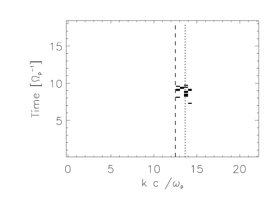
Figure 11: Temporal evolution of the parallel electric field amplitude $E_{z}$ for different wave numbers. Dark corresponds to locations where the amplitude exceeds the average field amplitude by $4\sigma$. Overplotted are the wave numbers for Langmuir waves generated by a parallel propagating weak beam with $v_{\|}/c=0.62$ (dotted) and $v_{\|}/c=0.66$ (dashed).

5.4 Proton Velocity Distribution

Figure 12: Projection of the protons in phase space to the plane $v_{x}$ vs. $z$ at $t=10.7\Omega_{p}^{-1}$. Contour levels are at $[1,10,100]$ particles. The ambient magnetic field points from left to right.

The initial proton velocity distribution is assumed to be isotropic at a temperature of $T^{p}=T_{\perp}^{e}$. Although protons do not contribute any free energy to the instability, they play a significant role in the course of the instability. As the growing wave due to the EFI is left hand polarized, the protons come in normal Doppler resonance with the wave. Unlike electrons, where only the high velocity tails of the distribution are affected by resonance, the resonance velocity for the protons lies within the bulk of the proton velocity distribution. Therefore the protons are expected to absorb energy from the wave. The non-collisional electron-proton coupling leads to a partial transfer of thermal energy from the electrons to the protons. This energy transfer was already conjectured by Hollweg and Völk (1970).

Due to the low thermal velocities of the protons, the gyroresonance velocity can be estimated in a non-relativistic limit, simplifying Eq. (3) to

$$v_{\|}=\frac{\omega-\Omega_{p}}{k}=\frac{\omega/\Omega_{p}-1}{kc/\omega_{p}}c_{A}$$ (5)

for resonance with an left hand polarized wave, where $c_{A}=c\Omega_{p}/\omega_{p}$ is the Alfvén-speed. The initially fastest growing waves $(kc/\omega_{p};\omega/\Omega_{p})=(0.88;0.68)$ and $(1.32;1.82)$ have resonance velocities $v_{\|}/v^{p}=-1.0$ and $1.8$. Both waves could be in resonance with some of the protons but due to the small amplitude of the waves, their influence is small.

Due to the isotropization of the electron velocity distribution, the wave frequencies at fixed wave number change and therefore the proton resonance velocities have changed to $v_{\|}/v^{p}=-2.1$ for $(0.88;0.33)$ and to $v_{\|}/v^{p}=0.2$ for $(1.32;1.07)$ at time $7.3\Omega_{p}^{-1}$. The resonance velocity for $kc/\omega_{p}=0.88$ is already far out in the proton velocity distribution and does not affect the proton velocity distribution any more. For the wave $(1.32;1.07)$ on the other hand, a large fraction of the proton distribution can be in resonance.

Figure 12 shows the proton distribution in a projection of phase space at $10.7\Omega_{p}^{-1}$. The spatial wave pattern corresponds to $kc/\omega_{p}=0.88$, which is not in resonance with the protons. The wave with $kc/\omega_{p}=1.32$ on the other hand is in resonance with the bulk of the proton velocity distribution, leading to pitch angle scattering of the protons towards larger $|v_{\perp}|$ while reducing $|v_{\|}|$.

6 Energy and Temperature Development

The transfer of free energy from the electrons to the protons through wave-particle interaction can be observed by considering the relevant energies in the simulated system.

Figure 13: Energy development per particle: Total energy $E^{f}+E^{k}_{p}+E^{k}_{e}$ (dotted), electron kinetic energy $E^{k}_{e}$ (solid), electromagnetic field energy $E^{f}$ (dash-dotted), proton kinetic energy $E^{k}_{p}$ (dashed), and $E^{f}+E^{k}_{p}$ (dashed, thin).

Figure 13 shows the development of the different energies per particle, demonstrating the transfer of free electron energy into waves and from there into proton kinetic energy. The kinetic energy of species $i$ is given by

$$E^{k}_{i}=\frac{1}{n_{p}}\sum\limits_{j=1}^{n_{p}}m_{p}c^{2}(\gamma_{j}-1),$$ (6)

where $\gamma_{j}$ is the Lorentz-factor of particle $j$. The electromagnetic field energy is given by

$$E^{f}=\frac{1}{2n_{p}}\int\!\!\!\int\!\!\!\int(E^{2}+c^{2}B^{2})dx\,dy\,dz,$$ (7)

where $E^{2}=E_{x}^{2}+E_{y}^{2}+E_{z}^{2}$ and $B^{2}=B_{x}^{2}+B_{y}^{2}+B_{z}^{2}$.

First it should be noted that throughout the simulated time the total energy is conserved to less than $2\%$.

Initially, an electron has on average a total energy of $\approx 25$ keV, with $23$ keV in parallel direction and $1$ keV in each perpendicular direction. The protons are initially isotropic with $1$ keV per proton in all directions.

Up to $\approx 10\Omega_{p}^{-1}$, the electron kinetic energy remains about constant. At the same time the parallel electron temperature is reduced significantly, thus most of the free energy is used to heat the electrons in perpendicular direction. However, some of the electron energy is converted into magnetic field energy. Due to the high mobility of the electrons, large scale electric fields do not build up. Between $10-12\Omega_{p}^{-1}$, energy goes mainly into the magnetic field. After saturation, the electron energy remains constant, indicating that the electrons play a passive role in the later development. This is also supported by the almost constant $E^{f}+E^{k}_{p}$.

The protons do not increase their energy significantly up to about $10\Omega_{p}^{-1}$. At that time, the bulk of the protons becomes resonant with the waves, increasing their kinetic energy at the cost of the wave. However, due to the resonant character of the interaction between protons and the waves, the proton kinetic energy can also be fed back into the magnetic field, leading to the oscillations seen after $t\Omega_{p}\approx 15$.

7 Real Plasmas

The isotropization process of an electron temperature anisotropy has been investigated in case of a plasma with $m_{p}/m_{e}=49$. What happens in a real plasma with $m_{p}/m_{e}=1836$? As shown in Fig. 4 and Fig. 5, the effect of an increased proton mass is wave growth at larger $k$. Additionally the maximum growth rate will be slightly larger.

The shift of the maximum growing wave number for reduced anisotropy, as well as the reduction of the wave frequencies at fixed wave numbers, will also occur in a plasma with real mass ratio. E.g. a reduction of the electron temperature ratio from $T^{e}_{\|}/T^{e}_{\perp}\approx 20$ to $T^{e}_{\|}/T^{e}_{\perp}\approx 6$ will shift the wave number of maximum growth from $kc/\omega_{p}=1.2$ to $kc/\omega_{p}=1.8$.

What happens to the protons? Keeping the ratio $\Omega_{e}/\omega_{e}$ constant, the Alfvén-speed $c_{A}$ has to be scaled by $\sqrt{m_{r}}$, where $m_{r}$ is the ratio between artificial and real proton mass. At the same time, the thermal velocity has to be scaled by $\sqrt{m_{r}}$, thus the ratio $v_{\|}/v^{p}$ remains constant. However, for a fixed wave number, the frequency decreases due to the different dispersion relation. It was shown in Sect. 5.4, that the fastest growing wave was in resonance with protons much slower than the thermal velocity. This is still true in case of a plasma with real mass ratio, e.g. for a temperature ratio of $T^{e}_{\|}/T^{e}_{\perp}\approx 6$, the fastest growing mode is $(kc/\omega_{p};\omega/\Omega_{p})=(1.7;0.9)$ and the resonance velocity is $v_{\|}/v^{p}=0.16$.

Due to the resonant absorption of the waves by the protons and the broader wave spectrum excited in a real plasma, the heating of the protons due to the EFI may be larger than predicted by the simulations. Additionally it was demonstrated in the previous section, that the absorption of field energy by the protons has only minor influence on the electrons. As the only drain of free electron energy is either isotropization or wave growth, and a broader spectrum of waves is excited in a real plasma, the simulated electron temperature isotropization time can be assumed to be an upper limit. Faster isotropization is confirmed by a simulation with increased mass ratio of $m_{p}/m_{e}=81$ (see Fig. 7).

8 Summary

The preferred acceleration along an external magnetic field compared to the perpendicular direction causes an unsolved problem in solar flare particle acceleration mechanisms. Without additional scattering mechanisms, this leads to an anisotropic electron velocity distribution, which can in turn reduce the efficiency of the accelerator. The isotropization time of an anisotropic velocity distribution has to be short compared to the total acceleration time which is $0.4$ s or less to energize the electrons to $20$ keV.

Based on linear theory, the Electron Firehose Instability (EFI) has been proposed as a candidate for velocity space particle scattering. In the previous sections, the temporal development of the EFI and its influence on the particle velocity distribution has been shown, based on self-consistent electromagnetic PIC simulations. The plasma parameters were chosen to be comparable to expected values in a solar flare plasma.

In case of a rod shaped geometry, which allows long-wavelength modes to grow mainly parallel to the external magnetic field, the process responsible for isotropization is identified to be the Electron Firehose Instability. The identification is made by comparison of the growth rate and the dispersion relation between simulations and linear theory.

The EFI is driven by the bulk of the electron velocity distribution, and is thus non-resonant. Most of the parallel electron energy is thereby converted into perpendicular electron energy. However, some free energy is converted into magnetic field energy.

The growing waves are left hand polarized electromagnetic waves with frequencies close to $\Omega_{p}$. As soon as the wave amplitudes are large enough, they start to scatter the electrons in velocity space by anomalous Doppler resonance. In this phase, the electrons emit most of their free energy as waves by reducing quickly their anisotropy. Wave growth stops after the anisotropy has been reduced below the instability criterion.

The strong waves generated by the instability mainly show up in the perpendicular magnetic field. Due to their left hand polarization, they are normal Doppler resonant with the protons. The resonance velocities of the waves generated by the EFI are in the bulk of the proton velocity distribution, and can thus be easily absorbed by the protons. This leads to perpendicular heating of the protons.

At the time of the anomalous Doppler resonance of the electrons with the wave, the electrons build up bumps in the reduced velocity distribution. They are the source of Langmuir waves, which in turn may yield observable radio emission.

Under solar flare conditions, the simulated plasma corresponds to a plasma with electrons of 2 keV in perpendicular direction and 23keV parallel to the external field. According to the simulations, this distribution isotropizes within about $20\Omega_{p}^{-1}$, corresponding to $2\cdot 10^{-5}{\rm s}$. The resulting isotropic energy of the electrons is about $7{\rm keV}$. The isotropization is fast compared to the timescales needed to accelerate the whole electron distribution to $25$keV, which is expected to be on many orders of magnitude larger time scales. The electron anisotropy originating from acceleration can therefore not be maintained.

Due to the large growth rates of the EFI at oblique angles, occurrence of the oblique firehose instability in a real plasma is even more likely. However, it is not yet clear how much energy is carried by those modes and what their influence on the particle distribution is. Additionally, due to the artificial mass ratio, the isotropization time may be overestimated. The given isotropization time due to the EFI can therefore be considered as an upper limit for an anisotropy to exist. Increasing computing resources will allow to tackle the problem in a slap shaped or even fully 3D geometry with larger mass ratios. This is the topic of current investigations.

In these simulations, most of the free energy is used to heat the electrons in perpendicular direction. Little energy goes into the protons, heating them in perpendicular direction and cooling them in parallel direction. The isotropization process can therefore not be used to explain bulk heating of the protons.

For the assumed plasma parameters, the Electron Firehose Instability limits the anisotropy. The particle distribution can therefore be assumed to be isotropic throughout the acceleration process.