Intrinsic Variability of the Vela Pulsar: Lognormal Statistics and Theoretical Implications

Abstract

Individual pulses from pulsars have intensity-phase profiles that differ widely from pulse to pulse, from the average profile, and from phase to phase within a pulse. Widely accepted explanations for pulsar radio emission and its time variability do not exist. Here, by analysing data near the peak of the Vela pulsar’s average profile, we show that Vela’s variability corresponds to lognormal field statistics, consistent with the prediction of stochastic growth theory (SGT) for a purely linear system close to marginal stability. Vela’s variability is therefore a direct manifestation of an SGT state and the field statistics constrain the emission mechanism to be linear (either direct or indirect), ruling out nonlinear mechanisms like wave collapse. Field statistics are thus a powerful, potentially widely applicable tool for understanding variability and constraining mechanisms and source characteristics of coherent astrophysical and space emissions.

1 Introduction

Pulsars are highly magnetized neutron stars whose rotation causes highly nonthermal beams of radiation to be swept across the Earth (Manchester & Taylor, 1977), similar to the periodic viewing of a lighthouse beam. Most likely the radio emission is produced over the star’s (magnetic) polar caps (Manchester & Taylor, 1977; Melrose, 1996; Asseo, 1996). Since their discovery in 1967 it has been recognized that only suitably long time averaging leads to a stable intensity profile versus pulsar phase. While this average profile is unique, individual pulses vary widely in intensity, often by a factor of $5$ or more, from one phase to another in a given pulse and from one pulse to the next at a given phase, as in Fig. 1. This variability (Manchester & Taylor, 1977; Hankins, 1996) includes phenomena known as drifting sub-pulses (Drake & Craft, 1968), microstructure (Craft et al., 1968), giant pulses (Cognard et al., 1996) and giant micropulses (Johnston et al., 2001). Sub-pulses are features which drift in time across the pulse window whereas microstructure are concentrated features superposed on a subpulse that are sometimes quasiperiodic. Giant pulses and micropulses are very rare pulses with fluxes $\stackrel{{\scriptstyle>}}{{\scriptstyle\sim}}10$ times the average flux (Cognard et al., 1996; Johnston et al., 2001). No accepted explanation exists for these forms of variability or, indeed, for the mechanism(s) producing pulsar radio emission (Manchester & Taylor, 1977; Melrose, 1996; Asseo, 1996; Hankins, 1996).

The high brightness temperatures of pulsars require coherent emission processes such as plasma microinstabilities or nonlinear processes. Linear mechanisms include (Melrose, 1996; Asseo, 1996; Luo & Melrose, 1995):(1) linear acceleration and maser curvature emission, in which electrons radiate coherently while accelerating in an oscillating large-scale field or on curved magnetic field lines, respectively, and (2) relativistic plasma emission, in which a streaming instability either directly generates escaping radiation near harmonics of the electron plasma frequency $f_{pe}$ or else drives localized (non-escaping) waves near $f_{pe}$ that are converted into escaping harmonic radiation by linear mode conversion or nonlinear processes. Nonlinear mechanisms can produce radiation by wave coalescence and scattering processes or as intense localized wavepackets, perhaps driven near $f_{pe}$ by a streaming instability, undergo modulational instabilities and strong turbulence wave collapse (Asseo et al., 1990; Asseo, 1996; Weatherall, 1998). Since existing analyses suggest that many mechanisms are viable, in part due to large uncertainties in the plasma properties and location of the emitting regions (e.g., above the polar cap or near the light cylinder), new approaches are necessary.

Analyses of intensity scintillations and angular broadening, corresponding primarily to Fourier analyses of data, are standard for astrophysical and solar system radiation sources (Rickett, 1990). In contrast, distributions of electric field strengths or intensities were rarely analyzed until recently, perhaps because their strong theoretical motivations and benefits were not clear before the advent of stochastic growth theory (SGT) (Robinson, 1992; Robinson et al., 1993; Cairns and Robinson, 1999; Cairns et al., 2000; Robinson and Cairns, 2001) and other theories like self-organized criticality (SOC) (Bak et al., 1987). However, recent analyses of 7 different solar system wave phenomena show that all have well-defined field distributions that agree very well with the predictions of SGT (Robinson et al., 1993; Cairns and Robinson, 1999; Cairns et al., 2000; Robinson and Cairns, 2001), resolving longstanding theoretical problems pertaining to the burstyness, widely varying fields, and persistence of the waves. Similarly, the giant pulses of some pulsars have power-law flux distributions (Cognard et al., 1996), sometimes interpreted qualitatively in terms of SOC (Young & Kenny, 1996). With the advent of rapid time resolution, coherently de-dispersed data for Vela and other pulsars (Johnston et al., 2001) the time is ripe for analyzing pulsar variability and its statistics in terms of SGT, SOC and other theories.

This paper directly addresses pulsar variability and emission mechanisms by analysing the radiation’s statistics near the peak of the Vela pulsar’s average profile and interpreting the results in terms of the theoretical predictions and formalism of SGT. After summarizing the predictions of SGT and other theories for wave growth (Section 2), Section 3 shows that Vela’s intrinsic variability near the peak of the average pulse profile corresponds to lognormal statistics in the electric field (or intensity), not Gaussian or power-law statistics in the intensity. Pulse variability is thus a direct manifestation of an SGT state. The consistency with the SGT prediction then strongly constrains the emission mechanism and source plasma (Section 4), with nonlinear emission mechanisms being non-viable in the phase range analysed. Preliminary results at other phases of Vela’s pulse profile and for other pulsars are then briefly discussed (Section 5). This analysis provides a first demonstration that radiation statistics for astrophysical sources are a powerful and potentially widely applicable tool for strongly constraining emission mechanisms and source plasmas.

2 Theories for Wave Statistics

Wave-particle interactions are expected to drive natural plasmas towards marginal stability, where wave emission and damping (as well as total energy inflow and outflow) are balanced. SGT treats systems in which an unstable particle distribution interacts self-consistently with its driven waves in an inhomogeneous plasma background and evolves to a state in which (i) the particle distribution is close to time- and volume-averaged marginal stability but with stochastic fluctuations that (ii) cause the wave gain $G$ to be a stochastic variable (Robinson, 1992; Robinson et al., 1993; Cairns and Robinson, 1999; Cairns et al., 2000; Robinson and Cairns, 2001). Here $G(t)$ is related to the wave growth rate $\Gamma(t)$ by $G(t)=\int_{-\infty}^{t}dt^{\prime}\Gamma(t^{\prime})$ and to the time-varying wave electric field $E(t)$ and a reference field $E_{0}$ by $E^{2}(t)=E_{0}^{2}\exp G(t)$. Rewriting this time integral as a summation over fluctuations $\Delta G_{i}=\Gamma_{i}\Delta t_{i}$ then, provided only that sufficiently many fluctuations in $\Delta G_{i}$ occur in some characteristic time, the Central Limit Theorem requires that $G(t)$ is a Gaussian random variable irrespective of the detailed distribution of $\Delta G_{i}$. Hypotheses (i) and (ii) thus have simple and natural physical justifications. The hypothesized random walk in $G\propto\ln E$ then implies that the waves should be bursty and widely varying in amplitude, while the closeness to marginal stability implies that the waves and driving distribution should persist far from the latter’s source. These characteristics are very attractive for pulsars, given the existence of intrinsic variability and the radiation’s broad bandwidth (and so large radial extension of the source inferred therefrom), as well for many other astrophysical and space phenomena.

Due to $G$ being a Gaussian random variable, pure SGT predicts that the probability distributions of wave field and intensity are lognormal (Robinson et al., 1993; Cairns and Robinson, 1999; Robinson and Cairns, 2001); i.e.,

$$P(\log E)=(\sqrt{2\pi}\ \sigma)^{-1}\exp(-(\log E-\mu)^{2}/2\sigma^{2})\ ,$$ (1)

where $\log$ means to the base $10$, $\mu$ and $\sigma$ are the average and standard deviation of $\log E$, respectively, and $\int d({\rm log}E)P(\log E)=1$. Nonlinear 3-wave processes active at high $E$ above a threshold $E_{c}$, which remove energy from the waves, reduce the $P(\log E)$ distribution below the prediction (1) near and above $E_{c}$ with known analytic form (Robinson et al., 1993; Robinson and Cairns, 2001). Processes like wave collapse and modulational instability cause a power-law tail with $P(E)\propto E^{-\alpha}$, with $\alpha$ ranging from $4$ to $6$, to develop above $E_{c}$ (Robinson, 1997; Robinson and Cairns, 2001). Waves driven from thermal levels by an instability, and which retain memory of their thermal past, also develop a power-law tail, but usually with a smaller index (Cairns et al., 2000; Robinson and Cairns, 2001). Finally, SOC should produce a power-law distribution with index close to $-1$ (Bak et al., 1987) and the usual model for wave growth in plasmas (uniform secular growth with constant growth rate) should produce a uniform distribution at fields below $E_{c}$ (Robinson et al., 1993; Cairns and Robinson, 1999; Robinson and Cairns, 2001). In contrast, scattering by density turbulence or radiation from multiple incoherently superposed sources is expected to produce Gaussian intensity distributions (Rickett, 1990). Rigorous testing of theories for wave growth is thus possible using the observed field statistics, as already demonstrated in multiple space contexts referenced above.

3 Statistics of Vela’s intrinsic variability

The data set consists of 20085 contiguous pulses (30 minutes) of the Vela pulsar, measured at 1413 MHz by the Parkes radio telescope and processed using coherent dedispersion and other techniques by Johnston et al. (2001). There are 2048 phase (time) bins per pulse period, each of $44\ \mu$s length (comparable to the scatter broadening time). Vela’s average intensity (over many pulses) is restored by adding $I_{0}=1250$ mJy to each sample. Fig. 1 shows the average pulse profile for relevant phase bins in mJy, together with $3$ superposed pulses which illustrate the variability. Note that the noise level is very low compared with earlier analyses, allowing detailed investigation of the intrinsic field statistics.

Analysis of data in the off-pulse phase bins lead to Gaussian statistics in the intensity $I$, as expected for instrumental and background noise. For instance, fitting the $P(I)$ distribution for phases 391-399 to a Gaussian, by using the Amoeba algorithm to minimize $\chi^{2}$ (Press et al., 1986), yields $\langle I\rangle=1215$ mJy (agreeing with $I_{0}$ to within less than the $100$ mJy bin width), $\sigma_{I}=1420$ mJy, $\chi^{2}=66$ for $N_{DF}=46$ degrees of freedom, and a significance probability $P(\chi^{2})=0.03$. (Fitting is restricted to intensity bins with $\geq 100$ pulse samples). This fit has good statistical significance.

Fig. 2 shows the $P(I)$ distribution and its best Gaussian fit for phase bin 490, close to the peak in Vela’s average profile. The fit clearly fails at both low and high $I$, entirely missing the long tail at large $I$, as confirmed by it having $\chi^{2}=301$ for $N_{DF}=53$ and $P(\chi^{2})<10^{-36}$. The variability at this phase is thus not described by Gaussian intensity statistics.

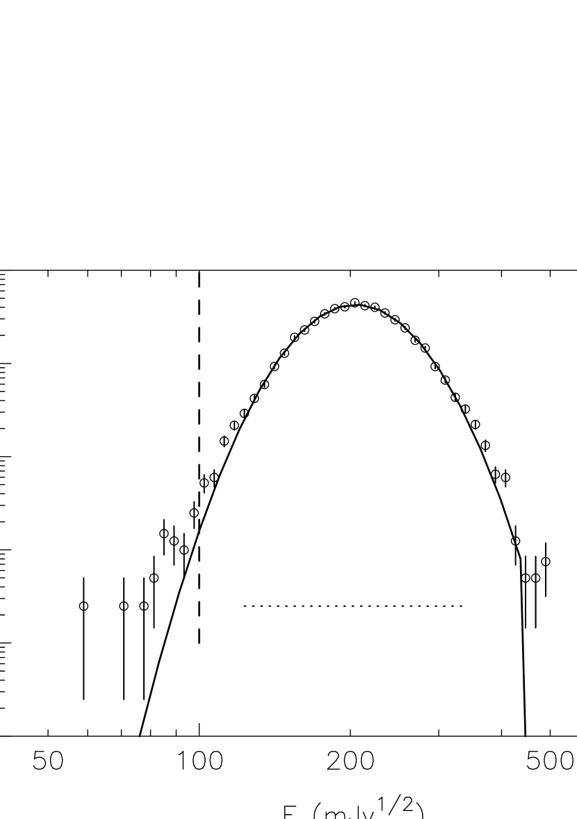
Figure 3: The observed distribution $P(\log E)$ at phase 490 (open circles and $\pm\sqrt{N}$ error bars), formed by binning the data linearly in $\log E$ and normalizing, is compared with the prediction (1) for lognormal field statistics. The symbols and dashed line are as in Figure 2.

In contrast, defining the electric field $E=I({\rm mJy})^{1/2}$, Fig. 3 shows that the $P(\log E)$ distribution for phase 490 is well fitted by the SGT prediction (1): for bins with $\geq 100$ pulse samples and $E\geq 10^{2}$ units (intensities above $10^{4}$ mJy, which is $6\sigma_{I}$ above the noise), $\mu=2.3$, $\sigma=0.096$, $\chi^{2}=27$ for $N_{DF}=19$, and $P(\chi^{2})=0.12$. The Kolmogorov-Smirnov test (Press et al., 1986) yields a significance probability of $47\%$. This fit is strongly statistically significant, clearly demonstrating that pulsar variability at this phase is lognormally distributed and quantitatively consistent with the theoretical form predicted by simple SGT. The fit matches the data well even outside the fitted range of fields (dotted line), although the effects of the noise background become increasingly evident at fields $\leq 80$ units.

Results similar to Fig. 3 are found for phases 485 - 540, for which the average pulsar intensity is well above the noise level, although the statistical significance varies. Rather than showing more results for individual phases, Fig. 4 shows the $P(X)$ distribution observed for phases 485 - 500 simultaneously, where $X=(\log E-\mu(\phi))/\sigma(\phi)$ is the field variable resulting from detrending variations in $\mu$ and $\sigma$ with phase $\phi$. Comparison with (1) shows that SGT predicts the $P(X)$ distribution to be Gaussian with zero mean and unit standard deviation (solid curve) (Cairns and Robinson, 1999). The agreement is very good, with the Kolmogorov-Smirnov test yielding a significance probability of $0.1\%$.

4 Theoretical Implications for Vela

For phases 485 - 540, where Vela’s average pulse profile is well above the noise, the field distributions do not have power-law tails or nonlinear cutoffs. Instead, the data have lognormal statistics and the variability is a direct manifestation of a simple SGT state, with no evidence for nonlinear processes, SOC, or uniform secular growth. This absence of a power-law tail or cutoff in the $P(\log E)$ distributions for these phases rules out pulsar emission mechanisms based on nonlinear processes (Asseo et al., 1990; Asseo, 1996; Weatherall, 1998) such as wave collapse, modulational instability, and three-wave processes. Instead, the observed consistency with simple (linear) SGT means that only linear emission mechanisms are viable, meaning that a plasma instability in a SGT state either directly generates the radiation or else generates non-escaping waves that are tranformed into escaping radiation by linear processes (e.g., mode conversion) alone.

From the definitions of $\mu$ and $\sigma$ and the intensity decreasing with distance $R$ as $R^{-2}$, it is easy to show that $\sigma(R)$ is constant and that $\mu(R)=\mu(R_{0})-\log(R/R_{0})$, where $\mu(R_{0})$ is the value at the source’s edge ($R=R_{0}$). Taking the values $\mu=2.0$ and $\sigma=0.1$ to be representative of these phases, the distance $R=350$ pc for Vela, and the value $R_{0}=30$ m, yields $\mu(R_{0})\approx 20$. The value $R_{0}=30$ m results from assuming that the overall source is annular, with radius equal to the neutron star radius $\approx 10$ km, and dividing by the $2048$ phase bins used for Vela. Accordingly, the ratio $\mu_{0}/\sigma\approx 200$ in the source. The values $\mu_{0}$ and $\sigma$ will constrain future theoretical models for why SGT applies.

5 Discussion and Conclusions

The foregoing analyses are the first applications of SGT to propagating EM radiation and, simultaneously, to extra-solar system sources. Their success implies that radiation statistics are an underappreciated and potentially very powerful tool in astrophysics (and space physics), and suggests that SGT may well be widely applicable to coherent astrophysical sources. As to whether the Vela results are representative of other pulsars, analyses are ongoing. Our results to date for pulsar PSR 1641-45, see also Johnston & Romani (2001), suggest that the variability near the peak of the average profile also corresponds to lognormal statistics, thereby being consistent with SGT and the Vela results above.

Of course, SGT is not likely applicable to all sources or indeed to all components of pulsar emissions. For instance, Jovian “S bursts” have a power-law flux distribution with index $2.0\pm 0.5$ (Queinnec & Zarka, 2001) and the peak flux distribution of solar microwave spikes can be fitted with an exponential or perhaps a lognormal form (Isliker & Benz, 2001). Moreover, this richness in possible wave statistics also appears in phase bins away from the peak in Vela’s average profile and for pulsars with giant pulses, where the observed $P(\log E)$ distributions are often approximately power-law. Detailed interpretations will be described in detail elsewhere. For now, we mention only that indices $\approx 4.5\pm 1.0$ are likely too high for SOC but are instead probably due to either driven thermal waves (Cairns et al., 2000) and/or due to strongly nonlinear processes like modulational instability and wave collapse (Robinson, 1997; Robinson and Cairns, 2001). The latter idea complements earlier suggestions (Asseo et al., 1990; Weatherall, 1998) and appears particularly attractive for giant pulses and giant micropulses.

In conclusion, analysis of rapidly-sampled, coherently de-dispersed data near the peak of the Vela pulsar’s average intensity-phase profile show that the field statistics are lognormal and quantitatively consistent with SGT’s prediction for a purely linear system near marginal stability. The variability is thus a direct manifestation of an SGT state and only linear emission mechanisms (either direct or indirect) are viable. Observations for other pulsars and at other phases for Vela yield both similar and different results, hinting at a possible richness of wave statistics and emission mechanisms. Analysis of field statistics is thus a powerful tool for understanding source variability and constraining the emission mechanisms and source characteristics that may be widely useful for coherent astrophysical and solar system radio emissions, as already found for plasma waves in space.

Figure 1: Average intensity-phase profile of the Vela pulsar for the dataset (thick solid line) together with three superposed individual pulses (other lines).

Figure 2: The observed distribution $P(I)$ at phase 490, formed by binning the data linearly in the intensity and normalizing by $\int dIP(I)=1$, is shown with open circles and $\pm\sqrt{N}$ error bars. The solid line shows the best-fit Gaussian, calculated for the domain shown by the dashed line.

Figure 4: The distribution $P(X)$ for all data in phases 485 – 500 (crosses), inclusive, is compared with the SGT prediction (solid line). See text for details.

References

- Asseo (1996) Asseo, E. 1996, in ASP Conf Ser. 105, Pulsars: Problems and Progress, ed. S. Johnston, M. A. Walker, & M. Bailes (San Francisco: ASP), 147
- Asseo et al. (1990) Asseo, E., Pelletier, G., and Sol, H. 1990, MNRAS, 247, 529
- Bak et al. (1987) Bak, P., Tang, C., and Weisenfeld, K. 1987, Phys. Rev. Lett., 59, 381
- Cairns and Robinson (1999) Cairns, I. H., and Robinson, P. A. 1999, Phys. Rev. Lett., 82, 3066
- Cairns et al. (2000) Cairns, I. H., Robinson, P. A., and Anderson, R. R. 2000, Geophys. Res. Lett., 27, 61
- Cognard et al. (1996) Cognard, I., Shrauner, J.A., Taylor, J.H., and Thorsett, S.E. 1996, ApJ, 457, L81
- Craft et al. (1968) Craft, H. D., Comella, J. M., and Drake, F. D. 1968, Nature, 218, 1122
- Drake & Craft (1968) Drake, F. D., and Craft, H. D. 1968, Nature, 220, 231
- Hankins (1996) Hankins, T. H. 1996, in ASP Conf. Ser. 105, Pulsars: Problems and Progress, ed. S. Johnston, M. A. Walker, & M. Bailes (San Francisco: ASP), 197
- Isliker & Benz (2001) Isliker, H., and Benz, A. 2001, A.&A., 375, 1040
- Johnston & Romani (2001) Johnston, S., and Romani, R. 2001, MNRAS, submitted
- Johnston et al. (2001) Johnston, S., van Straten, W., Kramer, M., and Bailes, M. 2001, ApJ, 549, L101
- Luo & Melrose (1995) Luo, Q., and Melrose, D.B. 1995, MNRAS, 276, 372
- Manchester & Taylor (1977) Manchester, R. N., and Taylor, J. H. 1977, Pulsars (San Francisco:Freeman), 281
- Melrose (1996) Melrose, D. B. 1996, in ASP Conf. Proc. 105, Pulsars: Problems and Progress, ed. S. Johnston, M. A. Walker, & M. Bailes et al. (San Francisco: ASP), 139
- Press et al. (1986) Press, W. H., Flannery, B. P., Teukolsky, S. A., and Vetterling, W. T. 1986, Numerical Recipes (New York, Cambridge)
- Queinnec & Zarka (2001) Queinnec J., and Zarka, P. 2001, Plan. Space Sci., 49, 365
- Rickett (1990) Rickett, B. J., 1990 Ann. Rev. Astron. & Astrophys., 28, 561
- Robinson (1992) Robinson, P.A. 1992, Sol. Phys., 139, 147
- Robinson (1997) Robinson, P.A. 1997, Rev. Mod. Phys., 69, 507
- Robinson and Cairns (2001) Robinson, P. A., and Cairns, I. H. 2001, Phys. Plasmas, 8, 2394
- Robinson et al. (1993) Robinson, P. A., Cairns, I. H., and Gurnett, D. A 1993, ApJ, 407, 790
- Weatherall (1998) Weatherall, J.C. 1998, ApJ, 506, 341
- Young & Kenny (1996) Young, M.D.T., and Kenny, B.G. 1996, in ASP Conf Ser. 105, Pulsars: Problems and Progress, ed. S. Johnston, M.A. Walker, & M. Bailes (San Francisco, ASP), 179