Extinction calculations of multi-sphere polycrystalline graphitic clusters

Certain dust particles in space are expected to appear as clusters of individual grains. The morphology of these clusters could be fractal or compact. In this paper we study the extinction by compact and fractal polycrystalline graphitic clusters consisting of touching identical spheres, based on the dielectric function of graphite from Draine & Lee (draine+lee (1984)). We compare three general methods for computing the extinction of the clusters in the wavelength range $0.1-100\leavevmode\nobreak\ \mu$m, namely, a rigorous solution (Gérardy & Ausloos GA (1982)) and two different discrete-dipole approximation methods – MarCODES (Markel markel (1998)) and DDSCAT (Draine & Flatau draine+flatau (1994)). We consider clusters of $N=$ 4, 7, 8, 27, 32, 49, 108 and 343 particles of radii either 10 nm or 50 nm, arranged in three different geometries: open fractal (dimension D $=1.77$), simple cubic and face-centred cubic. The rigorous solution shows that the extinction of the fractal clusters, with $N\leq 50$ and particle radii 10 nm, displays a peak within 2% of the location of the observed interstellar extinction peak at $\sim 4.6\mu$m^-1; the smaller the cluster, the closer its peak gets to this value. By contrast, the peak in the extinction of the more compact clusters lie more than 4% from $4.6\mu$m^-1. At short wavelengths ($0.1-0.5\mu$m), all the methods show that fractal clusters have markedly different extinction from those of non-fractal clusters. At wavelengths $>5\mu$m, the rigorous solution indicates that the extinction from fractal and compact clusters are of the same order of magnitude. It was only possible to compute fully converged results of the rigorous solution for the smaller clusters, due to computational limitations, however, we find that both discrete-dipole approximation methods overestimate the computed extinction of the smaller fractal clusters.

1 Introduction

The shape of interstellar and circumstellar grains is still an outstanding issue. For many years, the complexity of the electromagnetic scattering problem to solve has limited the shapes studied to spheres, infinite cylinders and spheroids. However, the shape of many interstellar grains are expected to be non-spherical and maybe even highly irregular. One way to deal with irregular particles and so with clusters of dust grains is to assume that they consist of touching spheres. With such an assumption it is possible to construct many distinct different morphologies which can then be compared with observations.

The problem of evaluating the extinction efficiency ($Q_{\rm ext}$) is that of solving Maxwell’s equations with appropriate boundary conditions at the cluster surface. A solution was formulated by Lorenz (lorenz (1890)) and Mie (mie (1908)) for a homogeneous single sphere and the complete formalism is therefore often referred to as Lorenz-Mie theory. A complementary solution based on expansion of scalar potentials was given by Debye (debye (1909)). A detailed description of this exact electromagnetic solution can be found in Bohren & Huffman (bohren+huffman (1983)). For a comprehensive review on the optics of cosmic dust see Voshchinnikov (nicolai02 (2002)).

An updated overview of exact theories and numerical techniques for computing the scattered electromagnetic field by clusters of particles is given in (Mishchenko et al. 2000a ; 2000b ; Fuller & Mackowski Fuller (2000); Ciric & Coorey Ciric (2000); Draine draine00 (2000); Voshchinnikov nicolai02 (2002) and references therein). All of these methods are based on solving Maxwell’s equations. For clusters of spheres embedded in non-absorbing media one such method is based on the Gérardy and Ausloos theory (Gérardy & Ausloos GA4 (1980); GA (1982); GA2 (1983); GA3 (1984)) which recently has been extended to also treat clusters embedded in absorbing media (Lebedev & Stenzel lebedev1 (1999); Lebedev et al. lebedev2 (1999)). Another method that is often used in practice is the discrete dipole approximation (DDA); it has been used in a wide range of scattering problems concerning clusters of particles including the extinction of interstellar dust grains (e.g. Vaidya et al. vaidya (2001); Bazell & Dwek bazell (1990)).

The Galactic interstellar extinction curve displays a “2175 Å peak”, which has presented an astrophysical puzzle since its discovery by Stecher (stecher (1965)). Fitzpatrick & Massa (fitzpatrick+massa86 (1986)) studied the interstellar extinction in the direction of 45 reddened stars, and found that it displays a peak whose central wavelength $\lambda_{0}$ is remarkably constant ($\lambda_{0}=2174.4\pm 17$ Å), even though its full width at half maximum (FWHM) varies considerably from $\leavevmode\nobreak\ 360$ to $\leavevmode\nobreak\ 600$ Å; they also found no apparent correlation between the small variation in $\lambda_{0}$ and the large variation in the FWHM.

Graphite has long been considered a very promising though controversial candidate for explaining the 2175 Å peak (e.g. Stecher & Donn stecher+donn (1965); Fitzpatrick & Massa fitzpatrick+massa (1988); Mathis mathis (1994); Voshchinnikov nicolai90 (1990); Sorell sorell (1990); Draine & Malhotra draine+malhotra (1993); Rouleau et al. rouleau (1997); Will & Aannestad will+aannestad (1999)). It is considered a promising candidate because small, 0.015 $\mu$m, graphitic spheres display an extinction peak at about the right wavelength with a FWHM in accordance with the observations (Gilra gilra (1972)), and because its abundance do not seem to contradict the cosmic abundance constraints (Snow & Witt snow+witt (1995)). It is considered a controversial candidate, however, because increasing the size of a small graphitic particle simultaneously increases the central wavelength and FWHM of its extinction peak. The peak will shift to longer wavelengths when the particle size is increased, when the particle shape is oblate spheroidal and when the particles are coated with a dielectric substance such as ice; it will shift to shorter wavelengths when the particle shape is prolate spheroidal (Gilra gilra (1972); Hecht hecht (1981); Draine & Malhotra draine+malhotra (1993)). The observed lack of correlation between the position and FWHM of the peak therefore presents a challenge to the hypothesis that graphite particles originate this peak. In an extensive investigation, Draine & Malhotra (draine+malhotra (1993)) conclude that if graphite particles are the carriers of the 2175 Å peak, a variation in their optical properties ought to be present. This may be the result of varying amounts of impurities, variations in crystallinity, or changes in its electronic structure due to surface effects. Clustering effects have also been considered; Rouleau et al. (rouleau (1997)) have shown that compact clusters of graphitic spheres satisfy the criterion that the position of the peak remain stable while the width varies.

To investigate the clustering effect further we here compute and analyse the extinction of different polycrystalline graphitic clusters. We have chosen clusters ranging from small to large, and that are either sparse or compact. In this way we intend to evaluate how the extinction is influenced by the structure. We focus on clusters consisting of 4, 7, 8, 27, 32, 49, 108 and 343 touching polycrystalline graphitic spheres. The extinction of the clusters is calculated by the use of a rigorous (GA) method (Gérardy & Ausloos GA (1982)) as well as by two DDA methods – MarCODES (Markel markel (1998)) and DDSCAT (Draine & Flatau draine+flatau (1994)) – to test how well these approximations perform when applied to clusters with different morphology. Recently Xu & Gustafson (xu+gustafson (1999)) compared light-scattering calculations by a rigorous solution similar to the GA method, with DDSCAT for two identical polystyrene spheres in contact. They found that DDSCAT worked reasonably well on small volume structures while its validity is challenged on large structures. We find a tendency for both the DDA codes to overestimate significantly the extinction for small (N $<10$) fractal clusters and to a much larger extent than for the comparable compact clusters.

By studying clusters consisting of polycrystalline graphitic particles we deal with the anisotropy of graphite in a different way than usual (e.g. Draine draine88 (1988)) and it turns out that this has an influence on the comparison of the calculated extinction with the observed interstellar extinction.

This paper is structured as follows. Section 2 deals with the anisotropy of graphite. Section 3 introduces the fractal and compact clusters studied in this work. Section 4 describes the computational methods under scrutiny; the exact GA solution (Gérardy & Ausloos GA (1982)) and the two different DDA methods, developed by Draine & Flatau (DDSCAT, draine+flatau (1994)) and Markel (MarCoDES, markel (1998)). Section 5 presents and dicusses our results for clusters from one up to 343 particles, in the wavelength range $0.03-100\leavevmode\nobreak\ \mu$m. Section 6 discusses the implications of our results in the interpretation of the interstellar extinction curve. Section 7 presents the conclusions.

2 Graphite

Theoretical computation of absorption and scattering by graphitic particles is difficult because graphite is a semi-metal with high anisotropy. Graphite can be characterised by two different dielectric functions, $\epsilon_{\perp}$ and $\epsilon_{\parallel}$, corresponding to the electric-field vector $\mathbf{E}$ being perpendicular ($\epsilon_{\perp}$) and parallel ($\epsilon_{\parallel}$) to the symmetry axis of the crystal ($c$-axis), which is perpendicular to the basal plane. It is a lot easier to experimentally determine $\epsilon_{\perp}$ than $\epsilon_{\parallel}$, because graphite cleaves readily along the basal plane and hence reflectivity measurements can be made with normally incident light, whereas it is very difficult to prepare suitable optical surfaces parallel to the $c$-axis.

In this work we deal with the anisotropy of graphite by assuming that in all our clusters, each individual particle is polycrystalline having a dielectric function $\epsilon_{\rm ave}$ given by the arithmetic average of $\epsilon_{\parallel}$ and $\epsilon_{\perp}$, namely $\epsilon_{\rm ave}=\frac{1}{3}\epsilon_{\parallel}+\frac{2}{3}\epsilon_{\perp}$. For a polycrystal, this arithmetic average is in fact an attainable upper bound for its dielectric function (Avellaneda et al. avellaneda (1988)). We use the dielectric functions $\epsilon_{\parallel}$ and $\epsilon_{\perp}$ derived by Draine & Lee (draine+lee (1984)) covering the region from the far-IR to the far-UV. The data agree well in the 0.03$-$62 $\mu$m region with those published by Borghesi & Guizzetti (borghesi+guizzetti (1991)).

In constrast, the usual “1/3$-$2/3” approximation, treats individual particles as mono-crystalline - 1/3 of the cluster particles are assumed to have dielectric function $\epsilon_{\parallel}$ and the remaining 2/3 to have dielectric function $\epsilon_{\perp}$. This approximation has been shown by Draine (draine88 (1988)) and Draine & Malhotra (draine+malhotra (1993)) to have a surprisingly good accuracy for graphite grains with radii $\leq 200$ Å. However, considering grain formation and grain growth in stellar environments (Sedlmayr sedlmayr (1994)), mono-crystalline particles do not seem to be as valid an assumption as polycrystalline ones. Also, investigations of presolar nano-diamond grains from meteorites - direct specimens of surviving physical material formed in past stellar environments which can be quantitatively analysed in the laboratory - show a clear tendency towards being polycrystalline (Daulton et al. daulton (1994); Phelps phelps (1999)).

Figure 1: The average dielectric function ($\epsilon_{ave}=\frac{2}{3}\epsilon_{\perp}+\frac{1}{3}\epsilon_{\parallel}$; see text) of graphite based on the dielectric functions derived by Draine & Lee (draine+lee (1984)).

A particle in vacuum will show a Lorenz-Mie absorption peak whenever the real part of its dielectric function, $\Re(\epsilon)$, satisfies $\Re(\epsilon)=-2$. Looking at the average dielectric function of graphite shown in Fig. 1, absorption peaks should occur at about $0.220\leavevmode\nobreak\ \mu$m and $14.6\leavevmode\nobreak\ \mu$m. The latter should be much more damped due to the higher value of the imaginary part of $\epsilon$.

3 Structure of the clusters

We consider three-dimensional clusters of identical touching spherical particles arranged in three different geometries: fractal, simple cubic, and face-centred cubic. The structures do not have shapes expected to be found in space, but will provide us with boundary conditions for the problem of calculating the extinction from clusters of grains of different morphology. Table 1 lists all the clusters used in this work.

Table 1: The clusters presented in this paper have three different geometries: fractal (frac; D$=1.77$), face-center cubic (fcc) and simple cubic (sc).

Cluster	# particles	Designation in
structure	in cluster	this paper
frac	7	frac7
frac	49	frac49
frac	343	frac343
fcc	4	fcc4
fcc	32	fcc32
fcc	49	fcc49
fcc	108	fcc108
sc	8	sc8
sc	27	sc27

The fractal clusters, frac7, frac49, and frac343, are obtained from the first three stages of the recursive construction of the snowflake fractal. This construction can be summarised as follows: a seed particle is put at the origin of the coordinate system. In the first step a generator is built by symmetrically gluing to the seed particle six copies of itself along the x, y, and z axes. Next, each particle in the first configuration, the generator, is substituted by the whole generator itself. In the next steps the same rule is applied: each particle is replaced by the generator. Fig. 2 shows this procedure up to the second stage. For a fractal cluster its dimension $D$ is defined by

$$M(r)=M_{0}\left[\frac{r}{r_{0}}\right]^{D},$$ (1)

where $M(r)$ is the mass of material contained within a sphere of radius $r$. For a solid grain of constant density $D=3$, whereas for a fractal grain $D<3$ (Mandelbrot mandelbrot (1983)); in particular, for the snowflake fractal $D={\rm ln7}/{\rm ln3}=1.77$ (Vicsek vicsek (1983)).

Although such a deterministic structure (Fig. 2) is not expected to occur in nature, its fractal dimension is close to that of more realistic random cluster-cluster aggregation models. In particular, small particles in space may move in straight, ballistic trajectories and form larger aggregates upon collisions. Numerical simulation of this process yields a value of around 1.9 for the fractal dimension of the resulting aggregates (Meakin meakin (1988); Botet and Jullien botet (1988); Meakin & Jullien meakin+jullien (1988)); this value has also been confirmed by experimental results (Wurm & Blum wurm (1998)). Moreover, optical properties of fractal clusters with $D<2$ are predicted to be significantly different from those with $D>2$ (Berry & Percival berry (1986)); hence we consider important to use a fractal with a realistic dimension in our computations. The open fractal structure presents a challenge for modelling due to the high porosity and large surface area.

As a contrast to the fractal structure, compact crystalline structures are studied, namely, face-centred cubic and simple cubic, see e.g. Kittel (kittel (1986)) for a discussion on crystal structures. All the clusters listed in Table 1 are symmetric except the fcc49. The non-fractal clusters are a challenge to model since they are far from being spherical.

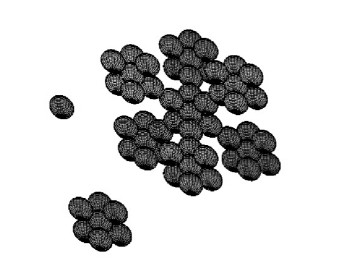
Figure 2: Stages of fractal construction. The seed particle, the generator (quasi-fractal clusters consisting of 7 particles) and the 3-D structure of the 49 particle fractal cluster (D$=1.77$), see text for more details.

4 The computational methods

4.1 Gérardy and Ausloos theory

A rigorous and complete solution to the multi-sphere light scattering problem has been given by Gérardy & Ausloos (GA) (GA4 (1980); GA (1982); GA2 (1983); GA3 (1984)) as an extension of the Mie-Ruppin theory (Mie mie (1908); Ruppin ruppin (1975)). It is based on the exact solution of Maxwell’s equations for arbitrary cluster geometries, polarisation and incidence direction of the light. This is done by expanding the various fields involved in terms of the vector spherical harmonics (VSH). The usual boundary conditions are extended to take into account the possible existence of longitudinal plasmons in the spheres. High-order multipolar electric and magnetic interaction effects are included. We summarise their work as used throughout the paper.

We consider a cluster of $N$ homogeneous spheres of radius $R$ and dielectric function $\epsilon(\omega)$, embedded in a matrix of dielectric constant $\epsilon_{M}$ and submitted to a plane polarised time harmonic electromagnetic field. The total scattered field from the cluster is represented as a superposition of individual fields scattered from each sphere. The electromagnetic field impinging on each sphere consists of the external incident wave and the waves scattered by the other spheres. For any sphere, the incident, internal and scattered fields are expressed in VSH centred at the sphere origin. The boundary conditions on its surface are solved by transforming all relevant field expansions into the sphere coordinate system, yielding the following system of linear coupled equations for the expansion coefficients $c_{\mu}$ and $d_{\mu}$ of the scattered field (Gérardy & Ausloos GA (1982)):

$$c_{\mu} =\Gamma_{q}\,\{\,{a_{0}}_{\mu}+\sum_{\nu}^{{}^{\prime}}(J_{\mu\nu}\ c_{\nu}+C_{\mu\nu}\ d_{\nu})\,\},$$ (2)

$$d_{\mu} =\Delta_{q}\{\,{b_{0}}_{\mu}+\sum_{\nu}^{{}^{\prime}}(C_{\mu\nu}\ c_{\nu}+J_{\mu\nu}\ d_{\nu})\,\},$$ (3)

where $\mu=(q,p,i)$ and $\nu=(n,m,j)$. The indices $q$ and $n$ denote the polar order, $p=-q,\dots,q,\ m=-n,\dots,n$, and the indices $i,j$ number the particles in the cluster. Moreover, ${a_{0}}_{\mu}$ and ${b_{0}}_{\mu}$ are the coefficients of the expansion of the external incident wave in VSH in the coordinate frame of the $i$ th sphere (Gérardy & Ausloos GA (1982)). The multi-polar electric and magnetic susceptibilities of a sphere (Gérardy & Ausloos GA (1982)) are denoted by $\Delta_{q}$ and $\Gamma_{q}$ respectively. The coefficients $J_{\mu\nu}$ and $C_{\mu\nu}$ describe the transformation of the VSH from a frame centred on particle $j$ to another centred on particle $i$. Analytical expressions for these coefficients have been given by Gérardy and Ausloos (GA (1982)). The primes in the sums in Eqs. (2) and (3) indicate that terms with $j=i$ are omitted. The solution to this system of equations can be written in matrix form as

$$\left[{\begin{array}[]{c}\mathbf{c}\\ \mathbf{d}\end{array}}\right]=\left[{\begin{array}[]{cc}\mathbf{T}_{N11}&\mathbf{T}_{N12}\\ \mathbf{T}_{N21}&\mathbf{T}_{N22}\end{array}}\right]\left[{\begin{array}[]{c}\mathbf{a_{0}}\\ \mathbf{b_{0}}\end{array}}\right],$$ (4)

where $\mathbf{T}_{N}$ is the T-matrix (Waterman waterman (1971); Tsang et al. tsang (1985); Mishchenko et al. 2000b ) of the cluster with components

$$\mathbf{T}_{N11} = (\,(\mathbf{\Gamma}^{-1}-\mathbf{J})-\mathbf{C}(\mathbf{\Delta}^{-1}-\mathbf{J})^{-1}\mathbf{C}\,)^{-1}$$ (5)

$$\mathbf{T}_{N12} = \mathbf{T}_{N11}\mathbf{C}\,(\mathbf{\Delta}^{-1}-\mathbf{J})^{-1}$$

$$\mathbf{T}_{N21} = (\mathbf{\Delta}^{-1}-\mathbf{J})^{-1}\mathbf{C}\,\mathbf{T}_{N11}$$

$$\mathbf{T}_{N22} = (\mathbf{\Delta}^{-1}-\mathbf{J})^{-1}(\mathbf{C}\,\mathbf{T}_{N12}+\mathbf{I}),$$

and $\mathbf{I}$ is the identity matrix. When $N=1$, Eq. (4) is just the Mie-Ruppin result (Mie mie (1908); Ruppin ruppin (1975))

$$\left[{\begin{array}[]{c}\mathbf{c}\\ \mathbf{d}\end{array}}\right]=\left[{\begin{array}[]{cc}\mathbf{\Gamma}&\mathbf{0}\\ \mathbf{0}&\mathbf{\Delta}\end{array}}\right]\left[{\begin{array}[]{c}\mathbf{a_{0}}\\ \mathbf{b_{0}}\end{array}}\right].$$ (6)

The extinction efficiency, $Q_{ext}$, i.e. the extinction cross-section in units of the total geometrical cross-section can then be obtained from Gérardy & Ausloos (GA (1982))

$$Q_{ext}=-\frac{1}{\pi Nk^{2}R^{2}}\,\Re(\mathbf{a}_{0}^{*T}\mathbf{c}+\mathbf{b}_{0}^{*T}\mathbf{d}),$$ (7)

where $k=2\pi/\lambda$ and $\lambda$ is the wavelength in the matrix. The extinction cross section per unit volume is then computed as

$$\frac{C}{V}=\frac{3}{4R}Q_{ext}.$$ (8)

Limiting $q$ and $n$ in Eqs. (2) and (3) to integers less than or equal to $L$, we obtain a system of $2NL(L+2)$ equations whose solution, Eq. (4), is the $2^{L}$-polar approximation to the electromagnetic response of the cluster; $\mathbf{a}_{0},\,\mathbf{b}_{0},\,\mathbf{c}\,\mbox{ and }\mathbf{d}$ are complex vectors of dimension $NL(L+2)$, while the $\mathbf{T}_{Nij},\,i,j=1,2$, are complex square matrices of dimension $NL(L+2)$. In this case Eqs. (7) and (8) determine the $2^{L}$-polar approximation to the cluster extinction efficiency and the cluster extinction per unit volume respectively.

The extension of this theory to treat the case of absorbing embedding media is given in (Lebedev & Stenzel lebedev1 (1999); Lebedev et al. lebedev2 (1999)).

4.2 The DDA method

The discrete dipole approximation (DDA) - also known as the coupled dipole approximation - method is one of several discretisation methods (e.g. Draine draine88 (1988); Hage & Greenberg hage+greenberg (1990)) for solving scattering problems in the presence of a target with arbitrary geometry. The discretisation of the integral form of Maxwell’s equations is usually done by the method of moments (Harrington harrington (1968)). Purcell & Pennypacker (purcell (1973)) were the first to apply this method to astrophysical problems; since then, the DDA method has been improved greatly by Draine (draine88 (1988)), Goodman et al. (goodman (1991)), Draine & Goodman (draine+goodman (1993)), Draine & Flatau (draine+flatau (1994)), Markel (markel (1998)), and Draine (draine00 (2000)). The DDA method has gained popularity among scientists due to its clarity in physical principle and the FORTRAN implementation which have been made publicly available by Draine & Flatau (DDSCAT package, Draine & Flatau draine+flatau (1994)) and by Markel (MarCoDES, Markel markel (1998)).

When considering the problem of scattering and absorption of linearly polarised light

$$E_{0}=e_{0}\exp\left(ikr\right)$$ (9)

by an isotropic graphitic grain, then within the concept of the DDA method, the grain is replaced by a set of discrete elements of volume $V_{i}$ with relative dielectric constant $\epsilon_{i}$ and dipole moments $d_{i}=d\left(r_{i}\right)$, $i=1,...,N,$ whose coordinates are specified by vectors $r_{i}$. The equations for the dipole moments can be written using simple considerations based on the concept of the exciting field, which is equal to the sum of the incident wave and the fields of the rest of the dipoles in a given point

$$\mathbf{d}_{i}\left(r_{i}\right)=\alpha_{i}\left[E_{0}\left(r_{i}\right)+k^{3}\sum_{j\neq i}\mathbf{G}_{ij}\mathbf{d}_{j}\left(r_{j}\right)\right]$$ (10)

where the dipole scattering tensor $\mathbf{G}_{ij}$ has the following form in dyad notations:

$$\mathbf{G}_{ij} = \left[A\left(kr\right)\delta_{ij}+B\left(kr\right)\frac{r_{i}r_{j}}{r^{2}}\right]$$ (11)

$$A\left(x\right) = \left[x^{-1}+ix^{-2}-x^{-3}\right]\exp\left(ix\right)$$

$$B\left(x\right) = \left[-x^{-1}-3ix^{-2}+3x^{-3}\right]\exp\left(ix\right)$$

$$\mathbf{r} \equiv \mathbf{r}_{ij}=\mathbf{r}_{i}-\mathbf{r}_{j}.$$

The solution of the set of Eqs. (10) and (11) yields all the basic optical characteristics of a particle such as the integrated extinction $\left(Q_{\rm ext}\right)$ and absorption $\left(Q_{\rm abs}\right)$:

$$Q_{\rm ext} = 4\pi k\Im\left[\sum_{i}\left(e_{0}d_{i}\right)\exp(-ik_{0}r_{i})\right]$$ (12)

$$Q_{\rm abs} = 4\pi k\sum_{i}\eta_{i}\left|d_{i}\right|^{2},\hskip 11.38092pt\eta_{i}=\frac{4\pi\Im\left(\epsilon_{i}\right)}{V_{i}\left|\epsilon_{i-1}\right|^{2}},$$

and scattering $\left(Q_{\rm sca}=Q_{\rm ext}-Q_{\rm abs}\right)$ efficiencies. Here $\Im$ means the imaginary part of the expression in the argument.

Once the location and polarisability of the points are specified, calculations of the scattering and absorption of light by the array of polarisable points can be carried out to in principle whatever accuracy is required. The limiting factor is the capacity of computing resources.

4.2.1 DDSCAT

In this work we use the DDSCAT code version 5a10 (Draine & Flatau draine+flatau (1994); Draine & Flatau draine+flatau00 (2000)). This version contains a new shape option where a target can be defined as the union of the volumes of an arbitrary number of spheres. In DDSCAT the considered grain/cluster is replaced by a cubic array of point dipoles. The cubic array has numerical advantages because the conjugate gradient method can be efficiently applied to solve the matrix equation describing the dipole interactions (Goodman et al. goodman (1991)). When knowing the dipole strength of each cell in the particle it is possible to compute the optical properties of arbitrary dust configurations.

There are three criteria for validity of DDSCAT:

1. The wave phase shift $\rho=|m|kd$ ($m=\sqrt{\epsilon}$ being the complex refractive index of the target material) over the distance $d$ between neighbouring dipoles should be less than 1 for calculations of total cross sections and less than 0.5 for phase function calculations.

2. $d$ must be small enough to describe the object shape satisfactorily.

3. The refractive index $m$ must fulfill $|m|<2$.

A comparison study by Draine & Flatau (draine+flatau (1994)) shows that scattering and absorption cross sections can be calculated with DDSCAT to accuracies of a few percent, provided that the criteria elaborated above are satisfied.

Xing & Hanner (xing+hanner (1997)) state that the $Q$ efficiency factor is generally much less sensitive to those criteria, and that it is usually sufficient to let the value of $\rho$ be around 1 or possible bigger. Xu & Gustafson (xu+gustafson (1999)) show through a comparison between the exact solution for two spheres in contact and DDSCAT that the criterion set up by Draine & Flatau (draine+flatau (1994)) is not sufficient to ensure high accuracy if the particles are large and strongly interacting (high refractive index). They, therefore, recommend to use a validity criteria of $\rho<0.3$ when calculating total cross sections.

The typical number of dipoles needed to obtain a reliable computational result using the DDSCAT code can be determined by calculating the minimum number of dipoles needed per particle. When a particle is represented by a 3-dimensional array of $N$ dipoles, its volume is $Nd^{3}$, which must be equal to $4\pi R^{3}/3$,

$$N=\frac{4\pi}{3}\left(\frac{R}{d}\right)^{3}=\frac{4\pi}{3}\left(\frac{2\pi R|m|}{\rho\lambda}\right)^{3}\approx 1039\left(\frac{R|m|}{\rho\lambda}\right)^{3}$$ (13)

since $d$ is related to the wave phase shift $\rho$ by $d=\rho/(|m|k)$ (Draine & Flatau draine+flatau00 (2000); Xing & Hanner xing+hanner (1997)). The number of dipoles needed to satisfactorily describe the shape of the object considered might be larger than indicated by Eq. (13) if the shape is “challenging”. It is important to remember that Eq. (13) only fulfills the first of the three criteria set by Draine & Flatau (draine+flatau00 (2000)).

For materials with large refractive index ($|m|>2$), Draine & Goodman (draine+goodman (1993)) show that especially the absorption is overestimated by DDA. The limitation in DDSCAT is set by the use of the lattice dispersion relation (LDR) for electromagnetic waves propagating on an infinite cubic lattice of point dipoles of polarisability $\alpha_{i}$ and spacing $d$. According to Draine & Goodman (draine+goodman (1993)), the LDR prescription for $\alpha_{i}$ gives fair accuracy for scattering but poorer results for absorption. When $|m-1|$ is large the continuum material is effective at screening the external field: in the limit $|m-1|\rightarrow\infty$ the internal field generated by the polarisation would exactly cancel the incident field, so that the continuum material in the interior of the target would be subjected to zero field. In the case of a discrete dipole array, the dipoles in the interior will also be effectively shielded, while the dipoles located on the target surface are not fully shielded and, as a result, absorb energy from the external field at an excessive rate. This error can be reduced to any desired level by increasing the number $N$ of dipoles, thereby minimising the fraction $\leavevmode\nobreak\ N^{-1/3}$ of the dipoles which are at surface sites, but very large values of $N$ are required when $|m|$ is large (Draine & Goodman draine+goodman (1993)).

Graphite is characterised by having a high refractive index. This means that the criterion $|m|<2$ is only fulfilled shortward of 0.072 $\mu$m ($m=n+ik=0.58+i1.42$) and relaxing the criterion a little (to account for the variability of $m$ that occurs) gives an upper limit of 0.216 $\mu$m ($m=0.66+i1.35$).

4.2.2 MarCoDES

Another efficient code based on DDA is the Markel Coupled Dipole Equation Solver (MarCoDES, Markel markel (1998)). This code is designed to solve the coupled Eq. (10) for an arbitrary cluster of $point$ dipoles using either conjugate gradient method (iterative method) or the LU expansion (direct method). The program is in principle applicable to clusters of small particles with arbitrary geometry, but is most computationally efficient for sparse clusters (i.e. when the volume fraction is very low) with significant number of particles $(\approx 10^{3}-10^{4})$. Contrary to DDSCAT the program does not use the Fast Fourier Transformation (FFT) because this might significantly decrease the computational performance for clusters with a low volume filling factor. When the volume filling fraction is close to unity, algorithms utilising FFT will be much faster. In the framework of the MarCoDES a spherical grain is considered to be equivalent to the single elementary dipole, this corresponds to $N=1$ in the DDSCAT case. The dimensionality of the coordinates of particles in MarCoDES require a special consideration. By replacing real particles by point dipoles located at their centres we significantly underestimate the strength of their interaction. In order to correct the interaction strength, the author of MarCoDES introduces geometrical intersection of particles. All coordinates are defined in terms of the distance between neighbouring dipoles $d$, which is given by $d=\left(4\pi/3\right)^{1/3}R$. So, for example, if two particles have radii 10 nm, then the distance between the dipoles is 16.12 nm. This suggested phenomenological procedure allows MarCoDES to be more accurate than the usual single dipole approximation since the intersection produces some analogy of including higher multipole interactions between particles. Application of MarCoDES to fractal sparse clusters allows, in principle, to introduce renormalisation on the sphere radii and number of particles depending on the fractal dimension of the cluster (Markel et al. markel00 (2000)), which will produce even further corrections to the strength. In this paper we use the simple particle intersection model given in the MarCoDES. The fact that the program only uses a single dipole for each particle in the cluster have significant benefits in computation efficiency when compared to other multi-polar approaches such as the GA method and DDSCAT.

5 Results

We present the results of the computation of the extinction of infrared, visible, and ultraviolet light by clusters of graphitic spheres of radii 10 nm and 50 nm, containing as few as 1 sphere to as many as 343 spheres. Specifically, our results concern the wavelength region from 0.1 to 100 $\mu$m. For convenience, we shall, from now onwards, call a cluster small if it has less than 10 particles, medium-size if it has between 25 and 50 particles, and large if it has more than 100 particles. With this convention, we shall first discuss the convergence of the GA computations, followed by a comparison of the three computational methods (GA, MarCoDES, and DDSCAT) when applied to the calculation of the extinction of a single polycrystalline graphitic sphere. Then we shall present in succession our results for small, medium-size, and large clusters, and end the section with an overall assessment of the computational methods in light of the results presented.

5.1 Convergence of GA method

As we stated in Sect. 4.1, with the GA method we can compute the extinction of a cluster in the $2^{L}$-polar approximation. We find that the smallest L needed for the convergence of the extinction of our clusters will be different for different regions of the optical spectrum. For small clusters, our full converged results show that in the UV-visible it is sufficient to use L = 7 for open clusters, and L = 9 for compact ones, to compute the extinction with an accuracy of 1%; whereas for longer wavelengths, at least L = 11 is required to ensure the same accuracy; this is so because in this region graphite has a metallic-like behaviour (high $|m|$), and, thus, higher order multipoles have to be included in the computation of the extinction to get the same accuracy as in the UV-visible range. We note that in the UV-visible range, by accepting an accuracy of 5% in the computation of the extinction, we can use L = 5 for open clusters and L = 7 for compact ones; we expect this to hold for clusters of up to a few tens of particles.

In column 2 of Table 2, we give the cut-off polar order L used in the calculation of the extinction of all our clusters. Full convergence was achieved only for small clusters; for the others, L indicates the maximum polar order obtained with our computer resources. In general, L = 11 was used for small clusters, L from 6 to 7 for medium-size clusters, and L from 2 to 3 for large clusters.

We show in Fig. 3 the convergence of the extinction of the frac7 cluster in the wavelength range $0.03-100\leavevmode\nobreak\ \mu$m. The inset shows the 2175 Å peak; around the peak maximum L = 3 already gives results accurate within 1%.

Figure 3: Solution of the GA method for the fractal cluster structure containing 7 polycrystalline graphitic particles. The solution is shown for different polar orders L. At L = 11 the solution was fully converged over the whole wavelength interval. The particle radius was 10 nm.

5.2 Single sphere

To set up a comparison baseline, we compute the extinction of af single sphere of radius 10 nm using the two DDA codes (DDSCAT and MarCoDES) and the GA solution. Since the GA theory extends that of Mie (Sect. 4.1), the GA and Mie solution coincide for a single sphere; this solution will be taken as a reference for the comparison.

It can be seen from Fig. 4 that DDSCAT is almost indistinguishable from the Mie solution for $\lambda\leq 1.0\leavevmode\nobreak\ \mu$m while MarCoDES is so for $\lambda\geq 0.6\leavevmode\nobreak\ \mu$m. The less good fit by DDSCAT for $\lambda>1.0\leavevmode\nobreak\ \mu$m is most likely a consequence of the refractive index of graphite having a modulus larger than 2 for these wavelengths, and of the 24 464 dipoles being inadequate to account for this.

Figure 4: A comparison between of DDSCAT, MarCoDES and the exact GA solution for a polycrystalline graphitic sphere with a 10 nm radius. The GA solution was fully converged at L = 2. The DDSCAT calculation was done with 24 464 dipoles.

5.3 Small ($N<10$) clusters

As before, we take the fully converged GA solutions as a reference for comparison. Fig. 5 shows the extinction of the frac7 cluster as computed with the three methods, while Fig. 6 shows similar information for the sc8 cluster. For the frac7 cluster (Fig. 5) MarCoDES underestimates the extinction for $0.2\leavevmode\nobreak\ \mu$m $<\lambda<0.25\leavevmode\nobreak\ \mu$m and systematically overestimates it for $\lambda>0.26\leavevmode\nobreak\ \mu$m. DDSCAT slightly underestimates the extinction for $\lambda<0.23\leavevmode\nobreak\ \mu$m and overestimates it for $\lambda>0.23\leavevmode\nobreak\ \mu$m. In the range $0.26\leavevmode\nobreak\ \mu$m $<\lambda<4\leavevmode\nobreak\ \mu$m the excess extinction from DDSCAT is smaller than for the MarCoDES calculations while for $\lambda>4\leavevmode\nobreak\ \mu$m DDSCAT gives a systematic relative increase in the excess extinction with wavelength which is much larger than the almost constant factor, $\sim 1.5$, seen for MarCoDES.

Figure 5: A comparison of the solutions from GA, MarCoDES and DDSCAT of the extinction cross section of the fractal cluster, shown in Fig. 2, consisting of 7 polycrystalline graphitic particles. The GA solution was fully converged at L = 11. In the DDSCAT calculation 6 838 dipoles were used. The particle radius was 10 nm.

For the sc8 cluster (Fig. 6) the trend is different. DDSCAT overestimates the extinction for $\lambda<0.3\leavevmode\nobreak\ \mu$m, underestimates it for $0.3\leavevmode\nobreak\ \mu$m $<\lambda<11\leavevmode\nobreak\ \mu$m and overestimates it again for $\lambda>11\leavevmode\nobreak\ \mu$m. MarCoDES also overestimates the extinction for $\lambda<0.26\leavevmode\nobreak\ \mu$m but then systematically underestimates it to a much larger extent than DDSCAT for $\lambda>0.26\leavevmode\nobreak\ \mu$m.

Figure 6: A comparison of the solutions from the GA, MarCoDES and DDSCAT calculations for the extinction cross section of the simple cubic cluster containing 8 polycrystalline graphitic particles. The GA solution was fully converged at L = 11. In the DDSCAT calculation 16 824 dipoles were used. The particle radius was 10 nm.

We have also investigated the effect of particle-size on a cluster’s extinction using the fully converged results of the GA solution. For this, in addition to the extinction of the frac7 cluster of spheres of radii 10 nm, we have also computed the extinction of a frac7 cluster of spheres of radii 50 nm; which was fully converged at L = 11 with a precision of 1.2%. Fig. 7 shows the results; what strikes the eye immediately is the high increase in the extinction over almost the entire wavelength range investigated, upon increasing the radii of the spheres. Still, for wavelengths $\lambda>1.1\leavevmode\nobreak\ \mu$m the shape of the extinction of both clusters look roughly the same. More important, however, are the differences observed in the wavelength range $\lambda<1.1\leavevmode\nobreak\ \mu$, where the extinction of the cluster with the larger spheres exhibits peaks at $0.11\leavevmode\nobreak\ \mu$m and $0.4\leavevmode\nobreak\ \mu$m in addition to the 2175 Å peak, which is the only peak displayed by the extinction of the cluster with the smaller spheres. All these observations agree with the finding of Kimura (2001) that the light scattering of fractal clusters depends strongly on the size parameter of the monomer.

Figure 7: The extinction cross section obtained with GA for frac7 with particle radius of 10 and 50 nm. The calculations were fully converged at L = 11.

5.4 Medium-size ($25<N<50$) clusters

Figure 8: A comparison of the solutions from GA, MarCoDES and DDSCAT for the extinction cross section of the frac49 cluster, shown in Fig. 2. The GA solution was truncated at L = 6. In the DDSCAT calculation 1 722 dipoles were used. The particle radius was 10 nm.

Figure 9: A comparison of the solutions from the GA, MarCoDES and DDSCAT calculations for the extinction cross section of the sc27 cluster. The GA solution was truncated at L = 7. In the DDSCAT calculation 16 783 dipoles were used. The particle radius was 10 nm.

Figure 10: A comparison of the solutions from the GA and DDSCAT calculations for the extinction cross section of the fcc32 cluster. The GA solution was truncated at L = 7. In the DDSCAT calculation 17 942 dipoles were used. The particle radius was 10 nm.

For the frac49 cluster, shown in Fig. 2, the extinction cross section obtained by the three methods is displayed in Fig. 8. For this structure neither DDSCAT nor MarCoDES gets close to the solution suggested from the GA calculations with L = 6. The GA solution is not fully converged at long wavelengths due to computational limitations; however, in the UV-visible region convergence is ensured at least with an accuracy of 5%. Both MarCoDES and DDSCAT greatly overestimates the extinction cross section for this cluster at longer wavelengths.

As a comparison to the frac49 cluster we have carried out calculations for two symmetric clusters, sc27 and fcc32, and an asymmetric one, fcc49.

For the sc27 cluster (Fig. 9) the GA solution was truncated at L = 7. MarCoDES underestimates the extinction for $0.17\leavevmode\nobreak\ \mu$m $<\lambda<0.22\leavevmode\nobreak\ \mu$m and $\lambda>0.29\leavevmode\nobreak\ \mu$m. DDSCAT also slightly underestimates the extinction for $0.17\leavevmode\nobreak\ \mu$m $<\lambda<0.22\leavevmode\nobreak\ \mu$m and $0.26\leavevmode\nobreak\ \mu$m $<\lambda<0.4\leavevmode\nobreak\ \mu$m, but systematically overestimates it for $\lambda>1\leavevmode\nobreak\ \mu$m.

We found that the version of MarCoDES tested here can not calculate a face-center cubic structure of touching particles because in this case the lattice cells representing neighbouring particles will touch only at the corners, giving as a consequence a spectrum corresponding to non-touching particles. The extinction of fcc32 and fcc49 clusters were therefore only calculated with the GA theory and DDSCAT. The results for fcc32 are displayed in Fig. 10; the results for the fcc49 cluster look similar. The GA calculations were truncated at L = 7 for fcc32 and at L = 6 for fcc49. For the DDSCAT calculations a $32\times 32\times 32$ dipole grid was used; for the fcc32 cluster this provides 17 942 dipoles ($\sim$ 561 dipoles per particle). For fcc49 a $48\times 32\times 40$ dipole grid was used; this provides 29 849 dipoles ($\sim$ 609 dipoles per particle). As can be seen in Fig 10, DDSCAT systematically overestimates the extinction especially at long wavelengths. The overestimation of the extinction cross section as calculated by DDSCAT is a general tendency for all the clusters we have studied. Also DDSCAT does not reproduce the absorption hump expected for graphite around $10-15\leavevmode\nobreak\ \mu$m, which is reproduced in the GA and MarCoDES calculations and also in Lorenz-Mie calculations by Draine & Li (draine+li (2001)).

5.5 Large ($N>100$) clusters

The GA solution could only be calculated to L = 3 for the fcc108 cluster and to L = 2 for the frac343 cluster due to computational limitations. The extinction of the fcc108 and frac343 clusters looks very similar to that of the fcc32 and frac49 clusters shown in Figs. 10 and 8, respectively. For the frac343 cluster the whole spectrum is shifted to longer wavelengths by about 0.002 $\mu$m and for the fcc108 cluster the whole spectrum is shifted 0.01 $\mu$m to longer wavelengths compared to the frac49 and fcc32 cluster, respectively. It was not possible to calculate these large clusters with DDSCAT.

5.6 Discussion

Figure 11: A comparison of the extinction cross section obtained with GA theory for the clusters frac49, fcc49, fcc32 and sc27. The 49 particle clusters were truncated at L = 6, while the two other clusters were truncated at L = 7. The particle radius was 10 nm.

It is seen that both DDA codes overestimate the extinction of the fractal structures at long wavelengths. A likely explanation is that the DDA model considers only point dipole interactions, whereas the GA solution matches the boundary conditions on the surface of the spherical particle and solves the problem of scattered and internal fields at the same time. Also, the large surface area of fractal clusters contributes to the complexity of the scattered field, which the GA method handles well because it takes into account the surface topology through the boundary conditions; the DDA codes, on the other hand, perform best when the surface to volume ratio is low. This interpretation is also supported by the calculations for the small compact sc8 cluster, see Fig. 6, where the DDA approximations perform reasonably well. For larger compact clusters, however, DDSCAT does not give good results at long wavelengths. This is due to computational limitations; the number of dipoles per particle that we could handle becomes lower as the cluster size increases. It is interesting to note that MarCoDES gives better results for compact than for fractal cluters of intermediate size. According to Markel et al. (markel00 (2000)), the performance of MarCoDES can be improved by altering the intersection parameter which determines if the particles touch or overlap, but we have not investigated that here. Nevertheless, the fact that MarCoDES in some cases overestimates the extinction, as compared to GA theory, and in other cases underestimates it, suggests that the determination of the rather arbitrary optimal intersection parameter is a very complex problem indeed.

We next compare the extinction of fractal and compact clusters of intermediate size. In Fig. 11, the GA calculation for frac49 is compared to that for fcc49 and fcc32. It is seen that the extinction of fractal and compact clusters are of the same order of magnitude. This is in contradiction to the DDA calculations which give a much higher extinction for fractal clusters (Figs. 5 - 11). We, therefore, recommend that great care should be taken when using these DDA codes at longer wavelengths for fractal clusters with low fractal dimension consisting of materials with high refractive index ($m$).

Concerning the effect of particle size on the extinction cross section, in classical electromagnetic theory the extinction is independent of cluster size in the long wavelength limit, i.e. when the size is much smaller than the wavelength. As seen in Fig. 7, clusters consisting of particles of radii 50 nm are clearly outside of this limit. Decreasing the particle radius below 10 nm, however, will give, in a classical theory, at most minor effects on the extinction of single particles and small clusters. Quantum mechanical effects, on the other hand, may influence the width and the position of the absorption peak for such small particles. A detailed study of these particle size effects on the extinction cross section is outside the scope of the present work.

6 The 2175 Å extinction peak

The main observational constraints concerning the 2175 Å peak are according to Fitzpatrick & Massa (fitzpatrick+massa86 (1986)) and Mathis (mathis (1994)):

1. The peak position is remarkably constant, $\nu_{\rm max}=4.6\pm 0.04\leavevmode\nobreak\ \mu$m^-1, where $\nu=1/\lambda$.

2. The peak width has a much larger range of variations of $1.0\pm 0.25\leavevmode\nobreak\ \mu$m^-1 (i.e. $\leq 25\%$).

3. The variation in peak position and the width ($\gamma$) are uncorrelated, except for the widest bumps ($\gamma\geq 1.2\leavevmode\nobreak\ \mu$m^-1) where a systematic shift to larger wavenumber is observed (Cardelli & Savage cardelli+savage (1988); Cardelli & Clayton cardelli+clayton (1991)). These later observations all have lines of sight passing through dark, dense regions.

Figure 12: Extinction cross section for polycrystalline graphitic clusters of different sizes calculated with the GA method. A difference in peak position can be seen between the fractal clusters and compact clusters. The lines in the plot indicate the peak position and width variation of the interstellar extinction curve. All clusters consist of particles with a 10 nm radius. Also shown is the GA solution for a sphere, radius 10 nm, which is equivalent to the Lorenz-Mie solution.

Table 2: Peak position and FWHM of different clusters, as calculated with the GA method. The value of L indicates at which polar order the GA calculations were truncated.

cluster name	L	peak	FWHM
		[$\mu$m-1]	[$\mu$m-1]
frac7	11	4.52	1.17
frac49	6	4.52	1.33
frac343	2	4.42	1.27
sphere	3	4.62	0.96
fcc4	11	4.43	1.15
fcc32	7	3.98	1.43
fcc 49	6	3.71	1.52
fcc108	3	3.98	2.01
sc8	11	4.41	1.27
sc27	7	4.12	1.62

Table 2 lists the peak position and width for the different cluster structures, as computed with the GA method. The polar order at which the GA calculation was truncated is also indicated. The width was determined as the FWHM. For the asymmetric compact cluster, we have investigated the importance of the orientation of the cluster and it was found that the peak position was shifted less than 0.1 $\mu$m^-1 while the width of the feature was not affected.

It was shown in a study by Rouleau et al. (rouleau (1997)), that small compact clusters qualitatively satisfy the observational constraints on the 2175 Å peak, except that the peak position falls at the wrong wavelength. This result is not confirmed from our findings, since the compact clusters we have studied do not have a stable peak position. The clusters considered by Rouleau et al. (rouleau (1997)) all had peak positions at higher wavenumber than the 2175 Å peak while the clusters we have considered all have peak position at lower wavenumbers. Rouleau et al. (rouleau (1997)) also used optical constants from Draine & Lee (draine+lee (1984)), but they dealt with the anisotropy of the graphitic particles with the usual “$1/3-2/3$” approximation, see Sect. 2, which assumes the particles to be mono-crystalline. As argued in Sect. 2 assuming the particles to be polycrystalline seems much more reasonable. This implies that variations in crystallinity is indeed an important factor when discussing the 2175 Å peak as also suggested by Draine & Malhotra (draine+malhotra (1993)).

The fractal clusters considered here do not enhance the long wavelength wing and do not introduce additional structure as seen by Rouleau et al. (rouleau (1997)) for elongated and ”fluffy” structures. The frac7 and frac49 clusters do come close (peak position is off by $0.04-0.08\leavevmode\nobreak\ \mu$m^-1) to the observational constraints. This indicates that small ($N\sim 5-100$) fractal clusters ought to be investigated in more detail to determine if fractal clusters with low fractal dimension have a stable peak position around $4.6\leavevmode\nobreak\ \mu$m^-1 and produce a variable width depending on the number of particles in the cluster.

7 Conclusions

We computed the extinction of clusters of polycrystalline graphitic particles in the wavelength range $0.1$ to $100\leavevmode\nobreak\ \mu$m. Computations by the rigorous multipolar theory of Gérardy & Ausloos (GA (1982); GA) were compared to two formulations of the discrete dipole approximation (DDA).

We have compared the extinction of open fractal clusters and compact clusters. The fractal and compact clusters display an extinction at long wavelengths, of the same order of magnitude as computed with the GA method. It seems that the DDA approximations grossly overestimate the long-wavelength extinction of small fractal structures. If this also holds true for larger fractal clusters is not possible for us to say due to computational limitations. The DDA codes should, however, be used with caution for this type of problem.

The GA computations were compared to the observed interstellar extinction curve. We found that results for small and medium-size (less than 50 particles) fractal clusters are in fair agreement with observational constraints, while those of compact sc and fcc clusters are not.

Convergence of the GA computations for small (less than 10 particles) clusters was found by including 11 multipoles. Good approximative results were obtained for medium-size (between 25 and 50 particles) clusters. In most cases we found a substantial differences between the GA theory and the DDA approximations of Draine & Flatau (draine+flatau (1994); DDSCAT) and Markel (markel (1998); MarCoDES).

As predicted by Draine & Goodman (draine+goodman (1993)) the absorption is significantly overestimated by DDSCAT at the wavelengths where the modulus of the refractive index, $|m|$, is large, see Figs. 8, 9 and 10. For $|m|<2$, DDSCAT performs well and better than the MarCoDES. MarCoDES, however, is computationally much faster than DDSCAT and the GA calculations. With DDSCAT the accuracy is directly dependent on the number of dipoles used in the approximation. Hence, by using more dipoles than we have used here, a better accuracy could be obtained, but then the computational cost would increase. Which DDA code is best to use will therefore depend on the type of problem one wants to address and the accuracy needed.

- (1) Avellaneda M., Cherkaev A.M., Lurie K.A. & Milton G.W., 1988, J. Appl. Phys. 63, 4989
- (2) Bazell D. & Dwek E., 1990, ApJ 360, 262
- (3) Berry M.V. & Percival I.C., 1986, Opt. Acta 33, 577
- (4) Bohren C.F. & Huffman D.R., 1983, Absorption and Scattering of Light by Small Particles (John Wiley & Sons, New York)
- (5) Borghesi A. & Guizzetti G., 1991, in Handbook of optical constants of solids II, ed. E.D. Palik (Academic Press, New York), 449
- (6) Botet R. & Jullien R., 1988, Ann. Phys. (France) 13, 153
- (7) Cardelli J.A. & Savage B.D., 1988, ApJ 345, 245
- (8) Cardelli J.A. & Clayton G.C., 1991, AJ 101, 1021
- (9) Ciric I.R. & Cooray F.R., 2000, in Light Scattering by Nonspherical Particles: Theory, Measurements and Applications, eds. M.I. Mishchenko, J.W. Hovenier, L.D. Travis (Academic Press, New York), 89
- (10) Daulton T.L., Eisenhour D.D., Lewis R.S & Bernatowicz T.J., 1994, Lunar Planet. Sci. 25, 313
- (11) Debye P., 1909, Ann. Phys. 30, 57
- (12) Draine B.T., 1988, ApJ 333, 848
- (13) Draine B.T., 2000, in Light Scattering by Nonspherical Particles: Theory, Measurements, and Applications, ed. M.I. Mishchenko, J.W. Hovenier & L.D. Travis (Academic Press, New York), 131
- (14) Draine B.T. & Flatau P.J., 1994, J. Opt. Soc. Am. A 11, 1491
- (15) Draine B.T. & Flatau P.J., 2000, User guide for the Discrete Dipole Approximation Code DDSCAT (Version 5a10), http://xxx.lanl.gov/abs/astro-ph/0008151v3
- (16) Draine B.T. & Goodman J.J., 1993, ApJ 405, 685
- (17) Draine B.T. & Li A., 2001, ApJ 554, 778
- (18) Draine B.T. & Lee H.M., 1984, ApJ 285, 89
- (19) Draine B.T. & Malhotra S.K., 1993, ApJ 325, 864
- (20) Fitzpatrick E.L. & Massa D., 1986, ApJ 307, 286
- (21) Fitzpatrick E.L. & Massa D., 1988, ApJ 328, 734
- (22) Fuller, K.A. & Mackowski, D.W, 2000, in Light Scattering by Nonspherical Particles: Theory, Measurements and Applications, eds. M.I. Mishchenko, J.W. Hovenier & L.D. Travis (Academic Press, New York), 225
- (23) Gérardy J.M. & Ausloos M., 1980, Phys. Rev. B 22, 4950
- (24) Gérardy J.M. & Ausloos M., 1982, Phys. Rev. B 25, 4204
- (25) Gérardy J.M. & Ausloos M., 1983, Phys. Rev. B 27, 6446
- (26) Gérardy J.M. & Ausloos M., 1984, Phys. Rev. B 30, 2167
- (27) Gilra D.P., 1972, in The Scientific Results of OAO-2, ed. A.D. Code (NASA, SP310), 295
- (28) Goodman J.J., Draine B.T. & Flatau P.J., 1991, Opt. Lett. 16, 1198
- (29) Hage J.I. & Greenberg J.M., 1990, ApJ 361, 251
- (30) Harrington R.F., 1968, Field Computation by Moment Methods, (Macmillan, New York)
- (31) Hecht J., 1981, ApJ 246, 794
- (32) Kimura H., 2001, Journal of Quantitative Spectroscopy & Radiative Transfer 70, 581
- (33) Kittel C., 1986, Introduction to Solid State Physics, (Wiley, New York), 11
- (34) Lebedev A.N. & Stenzel O., 1999, Eur. Phys. J. D 7, 83
- (35) Lebedev A.N., Gartz M., Kreibig U. & Stenzel O., 1999, Eur. Phys. J. D 6, 365
- (36) Lorenz L., 1890, Vidensk. Selsk. Skr. T. VI(6), (Bianco Lunos Kgl. Hof-Bogtrykkeri, Copenhagen), 1
- (37) Mandelbrot B.B., 1983, The Fractal Geometry of Nature (Freeman, San Francisco)
- (38) Markel V.A., 1998, User guide for MarCoDES - Markel’s Coupled Dipole Equation Solvers, http://atol.ucsd.edu/ pflatau/scatlib/
- (39) Markel V.A., Shalaev V.M. & George T.F., 2000, in Optics of Nanostructured Materials, eds. V.A. Markel & T.F. George (Wiley, New York), 355
- (40) Mathis J.S., 1994, ApJ 422, 176
- (41) Meakin P., 1988, Ann. Rev. Phys. Chem. 39, 237
- (42) Meakin P. & Jullien R., 1988, J. Chem. Phys. 89, 246
- (43) Mie, G., 1908, Ann. Phys. Leipz. 25, 377
- (44) Mishchenko M.I., Wiscombe W.J, Hovenier J.W. & Travis L.D., 2000a, in Light Scattering by Nonspherical Particles: Theory, Measurements and Applications, eds. M.I. Mishchenko, J.W. Hovenier & L.D. Travis (Academic Press, New York), 29
- (45) Mishchenko M.I., Travis L.D. & Macke A., 2000b, in Light Scattering by Nonspherical Particles: Theory, Measurements and Applications, eds. M.I. Mishchenko, J.W. Hovenier & L.D. Travis (Academic Press: New York), 147
- (46) Phelps A.W., 1999, Lunar Planet. Sci. 30, 1749
- (47) Purcell E.M. & Pennypacker C.R., 1973, ApJ 186, 705
- (48) Rouleau F., Henning Th. & Stognienko R., 1997, A&A 322, 633
- (49) Ruppin R., 1975, Phys. Rev. B 11, 2871
- (50) Sedlmayr E., 1994, in Molecules in the Stellar Environment, LNP 428, ed. U.G. Jørgensen (Springer, Berlin), 163
- (51) Snow T.P. & Witt A.N., 1995, Sci. 270, 1455
- (52) Sorell W.H., 1990, MNRAS 243, 570
- (53) Stecher T.P., 1965, ApJ 142, 1683
- (54) Stecher T.P. & Donn B., 1965, ApJ 142, 1681
- (55) Tsang L, Kong J.A. & Shin R.T., 1985, Theory of Microwave Remote Sensing (Wiley, New York), chapter 3
- (56) Xing, Z. & Hanner M.S., 1997, A&A 324, 805
- (57) Xu Y-L. & Gustafson B.Å.S., 1999, ApJ 513, 894
- (58) Vaidya D.B., Gupta R., Dobbie J.S. & Chylek P., 2001, A&A 375, 584
- (59) Vicsek T., 1983, J. Phys. A 16, L647
- (60) Voshchinnikov N.V., 1990, Sov. Astron. Lett. 16, 215
- (61) Voshchinnikov N.V., 2002, Astroph. & Space Sci. Rev. 12, 1
- (62) Waterman P.C., 1971, Phys. Rev. D 3, 825
- (63) Will L.M. & Aannestad P.A., 1999, ApJ 526, 242
- (64) Wurm G. & Blum J., 1998, Icarus 132, 125