Tidally distorted accretion discs in binary stars

Abstract

The non-axisymmetric features observed in the discs of dwarf novae in outburst are usually considered to be spiral shocks, which are the non-linear relatives of tidally excited waves. This interpretation suffers from a number of problems. For example, the natural site of wave excitation lies outside the Roche lobe, the disc must be especially hot, and most treatments of wave propagation do not take into account the vertical structure of the disc.

In this paper I construct a detailed semi-analytical model of the non-linear tidal distortion of a thin, three-dimensional accretion disc by a binary companion on a circular orbit. The analysis presented here allows for vertical motion and radiative energy transport, and introduces a simple model for the turbulent magnetic stress. The $m=2$ inner vertical resonance has an important influence on the amplitude and phase of the tidal distortion. I show that the observed patterns find a natural explanation if the emission is associated with the tidally thickened sectors of the outer disc, which may be irradiated from the centre. According to this hypothesis, it may be possible to constrain the physical parameters of the disc through future observations.

1 Introduction

1.1 Tidal effects on accretion discs

Accretion discs are commonly found in interacting binary star systems where matter is transferred from a normal star towards a compact companion (e.g. Lubow & Shu 1975). Tidal forces have an important role in these systems. The binary orbit is usually made accurately circular by the tidal interaction between the stars. The disc surrounding the compact star also experiences a strong tidal force from the companion, resulting in a non-axisymmetric distortion of the disc. Angular momentum transported outwards through the disc by ‘viscous’ stresses is transferred to the binary orbit through tidal torques.

The tidal interaction between a disc and an orbiting companion is also important in young binary stars and protoplanetary systems (e.g. Lin & Papaloizou 1993). In these situations there may be discs both interior and exterior to the companion’s orbit, which need not be circular.

Early theoretical studies addressed the tidal influence of a companion with a circular orbit and a mass ratio $q=M_{2}/M_{1}$ of order unity on a circumstellar disc (Paczyński 1977; Papaloizou & Pringle 1977). The method of Paczyński (1977) makes use of the idea that, in a thin accretion disc, the effects of pressure and viscosity are relatively weak. In the absence of resonances, and provided that the trajectories do not intersect, the motion of the gas is essentially ballistic. The ballistic trajectories in a circular binary system are just the orbits of the restricted three-body problem, which has been studied in great detail in celestial mechanics (e.g. Szébehely 1967). Paczyński (1977) showed that there is a family of these orbits that lie in the binary plane and are periodic in the binary frame, enclosing the compact star (Fig. 1). They reduce to circular Keplerian orbits when the companion star is removed. It is therefore natural to suppose that the streamlines of a tidally distorted disc correspond accurately to Paczyński’s orbits. The maximum size of the disc can be identified as the largest non-intersecting orbit.

Figure 1: Paczyński’s orbits in the restricted three-body problem for a mass ratio $q=1$. The prograde circumstellar case is depicted.

An alternative way of analysing the tidal distortion of a disc is through linear perturbation theory. A solution is first obtained for an axisymmetric disc around an isolated star. The tidal force is introduced as a perturbation and the linearized equations are solved to determine the tidal distortion. A solution can be found that is steady in the binary frame. The distortion of the disc is very slightly out of phase with the tidal forcing owing to the effective viscosity of the disc. This results in a tidal torque that increases with increasing radius until it becomes comparable to the local viscous torque and the disc is truncated. Such a calculation was carried out for a two-dimensional disc model by Papaloizou & Pringle (1977). At least for mass ratios of order unity, the tidal truncation radii determined by the two methods agree reasonably well.

1.2 Resonances

Additional complications arise if the disc contains radii at which the tidal forcing resonates with a natural mode of oscillation of the disc. For mass ratios $q\la 0.25$, a band of Paczyński’s orbits around the 3:1 resonance are parametrically destabilized (Hirose & Osaki 1990). In a continuous disc this causes a local growth of eccentricity (Lubow 1991), which may be able to compete with dissipative processes to sustain a global eccentric mode of the disc, as observed in superhump binaries.

When the mass of the companion is much smaller, one or more Lindblad resonances may be reached before the disc is truncated. Such resonances usually result in the launching of non-axisymmetric waves (Goldreich & Tremaine 1979). Unless the waves are able to propagate a significant distance through the disc, the torque exerted at a Lindblad resonance is localized and independent of the viscosity. Such a localized torque will often truncate the disc in the case of a very low-mass companion (e.g. Lin & Papaloizou 1986).

1.3 Three-dimensional effects

The methods of Paczyński (1977) and Papaloizou & Pringle (1977) both neglect the three-dimensional nature of the disc. In a linear analysis, Lubow (1981) has shown that the vertical component of the tidal force induces homogeneous vertical expansions and contractions of the disc, which are characterized by a vertical velocity proportional to the distance $z$ from the mid-plane. The natural frequency of this mode of oscillation, which corresponds to the $n=1$ p mode in the notation of Lubow & Pringle (1993), or the ${\rm p}_{1}^{\rm e}$ mode in the classification of Ogilvie (1998), depends on the adiabatic exponent $\gamma$.

As in the case of horizontal forcing, the response to vertical tidal forcing may involve resonant and non-resonant components. The equivalent of a Lindblad resonance for the ${\rm p}_{1}^{\rm e}$ mode is a vertical resonance, the location of which depends on $\gamma$ (Lubow 1981). If such a resonance lies within the disc, a resonant torque is exerted there and waves may be excited. Vertical resonances in a thin disc in a binary system are intrinsically much weaker than Lindblad resonances. However, for mass ratios of order unity, the $m=2$ inner vertical resonance typically lies within the tidal truncation radius, while the Lindblad resonances all lie well outside the disc (outside the Roche lobe, in fact). The vertical resonance can therefore have an important influence on the disc.

There is also a non-resonant, non-wavelike response to vertical tidal forcing at all radii. Dissipation can result in a significant phase shift in this response, causing an additional non-resonant tidal torque.

Although these effects have been widely neglected in the literature, Stehle & Spruit (1999) have recently proposed an interesting method of including vertical motion, in an approximate way, in two-dimensional numerical simulations of accretion discs. Stehle & Spruit (1999) also drew attention to the resonant excitation of vertical oscillations by the $m=2$ component of the tidal potential.

1.4 Non-axisymmetric structure in accretion discs

In recent years, non-axisymmetric features have been detected in the discs of several dwarf novae in outburst using Doppler tomography (Steeghs, Harlaftis & Horne 1997; Steeghs 2001 and references therein). The tomograms indicate the surface brightness of the disc, in the selected emission line, in a two-dimensional velocity space. The pattern generally appears as two crescents forming a broken ring, and the same is true when the pattern is mapped into real space, if circular Keplerian motion is assumed.

Steeghs et al. (1997) interpreted the non-axisymmetric features as evidence of ‘spiral structure’, ‘spiral waves’ or ‘spiral shocks’ in the disc. Observers of similar features in other systems have confidently reported them as spiral shocks (Joergens, Spruit & Rutten 2000; Groot 2001). Nevertheless, owing to the substantial complications in predicting line emission from cataclysmic variable discs (e.g. Robinson, Marsh & Smak 1993), these identifications should be regarded with some caution. The tomograms may not accurately reflect the dynamics of the disc, because they originate in the tenuous layers of the atmosphere. It might even be questioned whether the observed features indeed resemble either a spiral or a wave.

Two-armed spiral shocks had previously been seen in two-dimensional numerical simulations of the formation of very hot accretion discs by Roche-lobe overflow (Sawada, Matsuda & Hachisu 1986). Spruit (1987) showed with an analytical model that they could allow accretion to occur in an essentially inviscid disc, although the accretion rate is very small in a thin disc. Spiral shocks in two-dimensional disc models can be understood as the non-linear relatives of linear acoustic–inertial waves (Larson 1990). A popular conception is that such waves are excited by tidal forcing at the outer edge of the disc and steepen into shocks as they propagate inwards. Although the $m=2$ inner Lindblad resonance lies outside the Roche lobe, it is sometimes considered to launch waves through its ‘virtual’ effect on the disc (Savonije, Papaloizou & Lin 1994).

However, an analysis of Lindblad resonances in three-dimensional discs (Lubow & Ogilvie 1998) indicates that the dominant wave that is launched is the fundamental mode of even symmetry, or ${\rm f}^{\rm e}$ mode. Only in a vertically isothermal disc does this mode behave like the waves in a two-dimensional disc model; in a thermally stratified disc the ${\rm f}^{\rm e}$ mode behaves like a surface gravity mode and has quite different propagational properties. Typically, it dissipates after travelling only a short distance from the Lindblad resonance (Lubow & Ogilvie 1998; Bate et al. 2001).

Moreover, as pointed out by Godon, Livio & Lubow (1998), spiral waves in a thin accretion disc tend to be tightly wound except near resonances. If the non-axisymmetric features are to be interpreted as a two-armed wave, then the observations indicate at most one radial wavelength. Either the wave is highly localized in the radial direction, or it is not tightly wound. As the Lindblad resonances lie well outside the Roche lobe in IP Peg, it is very difficult to account for unwound waves in two-dimensional disc models unless the disc is unrealistically hot.

1.5 Vertical resonances

However, as mentioned by Godon et al. (1998), a vertical resonance could lie inside the disc in IP Peg. In fact, the location of the $m=2$ inner vertical resonance for an adiabatic exponent $\gamma=5/3$ agrees well with the observed features. In an inviscid, linear theory a ${\rm p}_{1}^{\rm e}$-mode wave is emitted from the resonance (Lubow 1981), which would not be tightly wound near the site of launching. However, in a separate paper (Ogilvie, in preparation) I make a detailed analysis of this resonance allowing for non-linearity and dissipation, and show that the resonance is typically saturated, broadened and damped to the extent that the emitted wave can be neglected. Therefore no such wave will be considered in the present paper. Nevertheless, the presence of the vertical resonance still has an important role in determining the tidal distortion, even if a wave is not generated.

1.6 Plan of the paper

The purpose of this paper is to determine the non-linear tidal distortion of a thin, three-dimensional accretion disc by a binary companion on a circular orbit. The fluid dynamical equations are solved in three dimensions by means of asymptotic expansions, using only the fact that the disc is thin. The resulting model is more complete than any previous analysis. Regarding the two-dimensional aspects of the problem, the model of Papaloizou & Pringle (1977) is extended by making it non-linear, while the model of Paczyński (1977) is developed by including the effects of pressure and turbulent stresses. In addition, allowance is made for vertical motion, radiative energy transport and stress relaxation. That is, a Maxwellian viscoelastic model of the turbulent stress is adopted, which accounts for the non-zero relaxation time of the turbulence.

This approach is part of the programme of ‘continuum celestial mechanics’ that has already addressed the dynamics of warped discs (Ogilvie 1999, 2000) and eccentric discs (Ogilvie 2001) using a closely related method. It provides a completely independent alternative to direct numerical simulations. The present method is more naturally suited to thin, but fully vertically resolved, discs. It also allows a more rapid solution, and is in some respects more advanced in physical content, than present-day simulations.

Although the finer details of the solutions obtained are not at present observationally testable, comparisons can be made at a simple level between the non-axisymmetric structure in the computed models and the features observed in Doppler tomograms. It will be seen that the observed patterns find a natural explanation if the emission is associated with the tidally thickened sectors of the outer disc, which may be irradiated from the centre.

The remainder of this paper is organized as follows. In Section 2 Paczyński’s orbits are used to define a orbital coordinate system that is used in solving the fluid dynamical equations. In Section 3 the model for the turbulent stress is explained. The basic equations are written in the orbital coordinate system in Section 4. The asymptotic development and solution of the equations is worked out in Section 5, leading to a prediction for the non-axisymmetric distortion of the disc. Simple synthetic Doppler tomograms are computed and compared with observations in Section 6. A summary and discussion of the results are found in Section 7.

2 Orbital coordinates

Consider a binary system with two stars in a circular orbit. The stars are approximated as spherical masses $M_{1}$ and $M_{2}$. Let $a$ be the binary separation and

$$\omega=\left[{{G(M_{1}+M_{2})}\over{a^{3}}}\right]^{1/2}$$ (1)

the binary orbital frequency.

Consider the binary frame rotating about the centre of mass with angular velocity $\omega$, and let $(R,\phi,z)$ be cylindrical polar coordinates such that star 1 (about which the disc orbits) is at the origin, while star 2 has fixed coordinates $(a,0,0)$. The axis of rotation passes through the centre of mass and is parallel to the $z$-axis. The Roche potential

$$\Phi=-GM_{1}(R^{2}+z^{2})^{-1/2}$$ (3)

$$-GM_{2}(R^{2}+a^{2}-2aR\cos\phi+z^{2})^{-1/2}$$

$$-{{1}\over{2}}\omega^{2}R^{2}+GM_{2}a^{-2}R\cos\phi$$

includes the gravitational potentials of the two stars and the centrifugal potential.

The analysis of a tidally distorted disc is simplified by introducing non-orthogonal orbital coordinates $(\lambda,\phi,z)$ based on Paczyński’s orbits, instead of cylindrical polar coordinates. The region of the binary plane filled by Paczyński’s orbits is covered by a coordinate system $(\lambda,\phi)$, where $\lambda$ is a quasi-radial coordinate that labels the orbits, and $\phi$ is the azimuthal angle. This naturally accounts for the principal tidal distortion of the disc. In this paper, only the case of a prograde circumstellar disc is considered, although the generalization to retrograde or circumbinary discs is straightforward.

There are many possible ways to label the orbits. In the case of eccentric discs (Ogilvie 2001) it was natural to use the semi-latus rectum, which measures the angular momentum of the orbits, and reduces to $R$ in the limit of circular orbits. However, the angular momentum is not constant on Paczyński’s orbits. A simple alternative is to define $\lambda$ to be the value of $R$ at $\phi=0$. In the absence of star 2, $\lambda$ reduces to $R$. In general, there exists a function $R(\lambda,\phi)$, satisfying $R(\lambda,0)=\lambda$, that defines the shape of the orbits and must be determined numerically.

To carry out the vector calculus required in the fluid-dynamical equations, one must obtain the metric coefficients and connection components (cf. Ogilvie 2001). The two-dimensional line element is

$${\rm d}s^{2}={\rm d}R^{2}+R^{2}\,{\rm d}\phi^{2}=(R_{\lambda}\,{\rm d}\lambda+R_{\phi}\,{\rm d}\phi)^{2}+R^{2}\,{\rm d}\phi^{2},$$ (4)

where the subscripts on $R$ stand for partial derivatives of the function $R(\lambda,\phi)$. Thus the metric coefficients are

$$g_{\lambda\lambda}=R_{\lambda}^{2},\qquad g_{\lambda\phi}=R_{\lambda}R_{\phi},\qquad g_{\phi\phi}=R^{2}+R_{\phi}^{2}.$$ (5)

As expected, the square root of the metric determinant is equal to the Jacobian of the coordinate system:

$$g^{1/2}=J={{\partial(x,y)}\over{\partial(\lambda,\phi)}}={{\partial(x,y)}\over{\partial(R,\phi)}}{{\partial(R,\phi)}\over{\partial(\lambda,\phi)}}=RR_{\lambda}.$$ (6)

The inverse metric coefficients are

$$g^{\lambda\lambda}={{R^{2}+R_{\phi}^{2}}\over{R^{2}R_{\lambda}^{2}}},\qquad g^{\lambda\phi}=-{{R_{\phi}}\over{R^{2}R_{\lambda}}},\qquad g^{\phi\phi}={{1}\over{R^{2}}}.$$ (7)

The components of the metric connection, given by

$$\Gamma^{a}_{bc}={\textstyle{{1}\over{2}}}g^{ad}(\partial_{b}g_{cd}+\partial_{c}g_{db}-\partial_{d}g_{bc}),$$ (8)

are found to be

$$\Gamma^{\lambda}_{\lambda\lambda}={{R_{\lambda\lambda}}\over{R_{\lambda}}},\qquad\Gamma^{\lambda}_{\lambda\phi}={{R_{\lambda\phi}}\over{R_{\lambda}}}-{{R_{\phi}}\over{R}},$$ (9)

$$\Gamma^{\lambda}_{\phi\phi}=-{{(R^{2}+2R_{\phi}^{2}-RR_{\phi\phi})}\over{RR_{\lambda}}},$$ (10)

$$\Gamma^{\phi}_{\lambda\lambda}=0,\qquad\Gamma^{\phi}_{\lambda\phi}={{R_{\lambda}}\over{R}},\qquad\Gamma^{\phi}_{\phi\phi}={{2R_{\phi}}\over{R}}.$$ (11)

The coordinate system is trivially extended to three dimensions by incorporating the vertical coordinate $z$. With the exception of $g_{zz}=g^{zz}=1$, all metric coefficients and connection components involving $z$ vanish. The three-dimensional Levi-Civita tensor (alternating tensor) is

$$\eta^{abc}=J^{-1}\epsilon_{abc},$$ (12)

where $\epsilon_{abc}$ denotes the usual permutation symbol with values $0,\pm 1$.

3 Modelling the turbulent stress

It is now widely accepted that the turbulent stress in most, if not all, accretion discs is magnetohydrodynamic (MHD) in origin, resulting from the non-linear development of the magnetorotational instability (Balbus & Hawley 1998). In MHD turbulence any fluid variable $X$ exhibits fluctuations $X^{\prime}$ about a mean value $\langle X\rangle$, so that $X=\langle X\rangle+X^{\prime}$ with $\langle X^{\prime}\rangle=0$. Correlations between fluctuating quantities result in a non-zero mean turbulent Maxwell stress tensor,

$${{1}\over{4\pi}}\bigg{\langle}B_{i}^{\prime}B_{j}^{\prime}-{{1}\over{2}}B_{k}^{\prime}B_{k}^{\prime}\,\delta_{ij}\bigg{\rangle},$$ (13)

and Reynolds stress tensor,

$$-\bigg{\langle}\rho u_{i}^{\prime}u_{j}^{\prime}+\rho^{\prime}(u_{i}u_{j}^{\prime}+u_{i}^{\prime}u_{j}+u_{i}^{\prime}u_{j}^{\prime})\bigg{\rangle}.$$ (14)

(In this section only, Cartesian tensor notation is used, together with the summation convention.) In numerical simulations the magnetic contribution is found to dominate and therefore any model of the stress should aim primarily to reflect the dynamics of the Maxwell tensor.

In a recent paper (Ogilvie 2001) I proposed a simple viscoelastic model of the turbulent stress in an accretion disc. This was put forward as a straightforward generalization of the standard viscous model, used extensively in accretion disc theory, to incorporate the effect of a non-zero relaxation time for the turbulence. It was also motivated by certain formal and physical analogies between MHD and viscoelasticity. Here I present a slightly refined version that accounts more completely for the transfer of energy between the mean motion and the turbulence, to heat and then to radiation.

The turbulent stress is written as $T_{ij}-{\textstyle{{1}\over{2}}}T_{kk}\delta_{ij}$, where $T_{ij}$ is a symmetric second-rank tensor that can be associated approximately with $\langle B_{i}^{\prime}B_{j}^{\prime}\rangle/4\pi$. The equation of motion is then

$$\rho(\partial_{t}u_{i}+u_{j}\partial_{j}u_{i})=-\rho\partial_{i}\Phi-\partial_{i}(p+{\textstyle{{1}\over{2}}}T_{jj})+\partial_{j}T_{ij},$$ (15)

where $\rho$ is the density, $u_{i}$ the velocity, $\Phi$ the external gravitational potential and $p$ the pressure. The tensor $T_{ij}$ is taken to satisfy the equation

$$T_{ij}+\tau{\cal D}T_{ij}=\mu(\partial_{i}u_{j}+\partial_{j}u_{i})-(2\mu_{\rm b}+{\textstyle{{2}\over{3}}}\mu)(\partial_{k}u_{k})\delta_{ij},$$ (16)

where $\tau$ is the relaxation time, $\mu$ the effective (dynamic) viscosity and $\mu_{\rm b}$ the effective bulk viscosity. The operator ${\cal D}$ is a convective derivative acting on second-rank tensors, and is defined by

$${\cal D}T_{ij}=(\partial_{t}+u_{k}\partial_{k})T_{ij}-T_{ik}\partial_{k}u_{j}-T_{jk}\partial_{k}u_{i}+2T_{ij}\partial_{k}u_{k}.$$ (17)

With the aid of the equation of mass conservation,

$$\partial_{t}\rho+\partial_{i}(\rho u_{i})=0,$$ (18)

an equation for the kinetic and gravitational energy of the fluid is then obtained in the form

$$\partial_{t}\left[\rho({\textstyle{{1}\over{2}}}u^{2}+\Phi)\right]+\partial_{i}\left[\rho({\textstyle{{1}\over{2}}}u^{2}+\Phi)u_{i}\right]$$ (19)

$$=-u_{i}\partial_{i}(p+{\textstyle{{1}\over{2}}}T_{jj})+u_{i}\partial_{j}T_{ij},$$

provided that $\Phi$ is independent of $t$. The turbulent energy density is identified as ${\textstyle{{1}\over{2}}}T_{ii}$ (which can be associated approximately with $\langle B_{i}^{\prime}B_{i}^{\prime}\rangle/8\pi$), and this satisfies the equation

$$\partial_{t}({\textstyle{{1}\over{2}}}T_{ii})+\partial_{i}(T_{jj}u_{i}-T_{ij}u_{j})=u_{i}\partial_{i}({\textstyle{{1}\over{2}}}T_{jj})-u_{i}\partial_{j}T_{ij}$$ (20)

$$-{{1}\over{\tau}}({\textstyle{{1}\over{2}}}T_{ii}+3\mu_{\rm b}\partial_{i}u_{i}),$$

obtained by taking the trace of equation (16). The first two terms on the right-hand side appear with the opposite sign in the preceding equation, and therefore represent the transfer of energy between the mean motion and the turbulence. The last term represents the loss of turbulent energy to heat. Accordingly the thermal energy equation is written as

$$\rho T(\partial_{t}s+u_{i}\partial_{i}s)={{1}\over{\tau}}({\textstyle{{1}\over{2}}}T_{ii}+3\mu_{\rm b}\partial_{i}u_{i})-\partial_{i}F_{i},$$ (21)

where $T$ is the temperature, $s$ the specific entropy and $F_{i}$ the radiative energy flux. The total energy then satisfies an equation of conservative form,

$$\partial_{t}\left[\rho({\textstyle{{1}\over{2}}}u^{2}+\Phi+e)+{\textstyle{{1}\over{2}}}T_{ii}\right]$$ (22)

$$+\partial_{i}\left[\rho({\textstyle{{1}\over{2}}}u^{2}+\Phi+h)u_{i}+T_{jj}u_{i}-T_{ij}u_{j}+F_{i}\right]=0,$$

where $e$ is the specific internal energy, which satisfies the thermodynamic relation ${\rm d}e=T\,{\rm d}s-p\,{\rm d}(1/\rho)$, and $h=e+p/\rho$ is the specific enthalpy.

Consider the following two limits of the above system. In the limit $\tau\to 0$ the stress is related instantaneously to the velocity gradient by

$$T_{ij}-{\textstyle{{1}\over{2}}}T_{kk}\delta_{ij}=\mu(\partial_{i}u_{j}+\partial_{j}u_{i})+(\mu_{\rm b}-{\textstyle{{2}\over{3}}}\mu)(\partial_{k}u_{k})\delta_{ij}.$$ (23)

The equation of motion then reduces exactly to the compressible Navier–Stokes equation. In the limit $\tau\to\infty$, however, the tensor $T_{ij}$ satisfies the equation

$${\cal D}T_{ij}=0,$$ (24)

which implies that $T_{ij}$ is ‘frozen in’ to the fluid. This is precisely the equation satisfied by the tensor $B_{i}B_{j}/4\pi$ when the magnetic field $B_{i}$ is ‘frozen in’ to the fluid according to the induction equation of ideal MHD. The system of equations therefore reduces exactly to ideal MHD in this limit.

For intermediate values of $\tau$, the viscoelastic model reproduces both the viscous (dissipative) and elastic (magnetic) characteristics of MHD turbulence. It is intended to give a fair representation of the dynamical response of the turbulent stress to a slowly varying large-scale velocity field as found in a tidally distorted disc. The use of a tensor $T_{ij}$ in this model, rather than a vector or scalar field, is essential in order to allow off-diagonal stress components. Apart from the radiative energy flux, which in this paper is treated in the diffusion approximation, the viscoelastic model for $\tau>0$ results in a hyperbolic system of equations and is therefore ‘causal’. It also satisfies the continuum mechanical principle of material frame indifference.

The viscoelastic model introduces a new dimensionless parameter for the disc. The Weissenberg number ${\rm We}$ can be defined as the product of the relaxation time and the angular velocity, and is expected to be of order unity, although it has never been measured directly. In the case of a circular, Keplerian disc the viscoelastic model predicts the usual ‘viscous’ stress component $T_{R\phi}=-{\textstyle{{3}\over{2}}}\mu\Omega$ plus an additional component $T_{\phi\phi}={\textstyle{{9}\over{2}}}{\rm We}\,\mu\Omega$. If the effective viscosity is given by an alpha prescription, $\mu=\alpha p/\Omega$, the quantity $T_{\phi\phi}$ can be associated approximately with a toroidal magnetic field with magnetic pressure ${\textstyle{{9}\over{4}}}{\rm We}\,\alpha$ times the gas pressure. The turbulent energy is stored in this component. The shear energy is tapped by the stress component $T_{R\phi}$, is converted into turbulent energy stored in $T_{\phi\phi}$, and then goes into heat and radiation.

4 Basic equations

The basic equations governing a fluid disc in three dimensions are now expressed in the orbital coordinate system.

The equation of mass conservation is

$$(\partial_{t}+u^{a}\nabla_{a})\rho=-\rho\nabla_{a}u^{a},$$ (25)

where now $u^{a}$ is the velocity relative to the rotating frame. The equation of motion is

$$\rho\left[(\partial_{t}+u^{b}\nabla_{b})u^{a}+2\eta^{abc}\omega_{b}u_{c}\right]$$ (26)

$$=-\rho\nabla^{a}\Phi-\nabla^{a}(p+{\textstyle{{1}\over{2}}}{T^{b}}_{b})+\nabla_{b}T^{ab},$$

where $\omega^{a}$ is the angular velocity of the rotating frame (only $\omega^{z}=\omega$ being non-zero).

As described above, the tensor $T^{ab}$ satisfies the equation

$$T^{ab}+\tau\left[(\partial_{t}+u^{c}\nabla_{c})T^{ab}-T^{ac}\nabla_{c}u^{b}-T^{bc}\nabla_{c}u^{a}+2T^{ab}\nabla_{c}u^{c}\right]$$ (27)

$$=\mu(\nabla^{a}u^{b}+\nabla^{b}u^{a})-(2\mu_{\rm b}+{\textstyle{{2}\over{3}}}\mu)(\nabla_{c}u^{c})g^{ab},$$

which, like the induction equation in MHD, is not affected by the rotation of the frame. The energy equation for an ideal gas is

$$\left({{1}\over{\gamma-1}}\right)(\partial_{t}+u^{a}\nabla_{a})p=-\left({{\gamma}\over{\gamma-1}}\right)p\nabla_{a}u^{a}$$ (28)

$$+{{1}\over{\tau}}({\textstyle{{1}\over{2}}}{T^{a}}_{a}+3\mu_{\rm b}\nabla_{a}u^{a})-\nabla_{a}F^{a},$$

where $\gamma$ is the adiabatic exponent. The radiative energy flux, in the Rosseland approximation for an optically thick medium, is given by

$$F^{a}=-{{16\sigma T^{3}}\over{3\kappa\rho}}\nabla^{a}T,$$ (29)

where $\sigma$ is the Stefan-Boltzmann constant and $\kappa$ the opacity. The equation of state of an ideal gas,

$$p={{k\rho T}\over{\mu_{\rm m}m_{\rm H}}},$$ (30)

is adopted, where $k$ is Boltzmann’s constant, $\mu_{\rm m}$ the mean molecular weight and $m_{\rm H}$ the mass of the hydrogen atom. The opacity is assumed to be of the Kramers form

$$\kappa=C_{\kappa}\rho T^{-7/2},$$ (31)

where $C_{\kappa}$ is a constant. The generalization to other power-law opacity functions is straightforward (Ogilvie 2000, 2001).

The effective viscosity coefficients are assumed to be given by an alpha parametrization. The precise form of the alpha prescription relevant to a tidally distorted disc is to some extent debatable. It will be convenient to adopt the form

$$\mu=\alpha p\left({{GM_{1}}\over{\lambda^{3}}}\right)^{-1/2},\qquad\mu_{\rm b}=\alpha_{\rm b}p\left({{GM_{1}}\over{\lambda^{3}}}\right)^{-1/2},$$ (32)

where $\alpha$ and $\alpha_{\rm b}$ are the dimensionless shear and bulk viscosity parameters. In the limit of a circular disc in the absence of star 2, this prescription reduces to the usual one, $\mu=\alpha p/\tilde{\Omega}$, etc., where $\tilde{\Omega}$ is the orbital angular velocity in the inertial frame. Finally, the Weissenberg number is defined by

$${\rm We}=\tau\left({{GM_{1}}\over{\lambda^{3}}}\right)^{1/2},$$ (33)

where $\tau$ is the relaxation time. Again, this reduces to ${\rm We}=\tilde{\Omega}\tau$ in the limit of a circular disc. For simplicity, the four dimensionless parameters of the disc, $(\alpha,\alpha_{\rm b},{\rm We},\gamma)$, will be assumed to be constant throughout this paper. The other parameter in the problem is the mass ratio $q=M_{2}/M_{1}$.

5 Solution of the equations

The analysis proceeds on the basis that the disc is almost steady in the binary frame, and evolves only on a time-scale (the viscous time-scale) that is long compared to the orbital time-scale. It is also assumed that the fluid variables vary smoothly in the horizontal directions, not on a length-scale as short as the semi-thickness of the disc. Under these conditions, the temporal and spatial separation of scales allows the fluid dynamical equations to be solved by asymptotic methods.

Let the small parameter $\epsilon$ be a characteristic value of the angular semi-thickness $H/R$ of the disc. Adopt a system of units such that the radius of the disc and the characteristic orbital time-scale are $O(1)$. Then define the stretched vertical coordinate $\zeta=z/\epsilon$, which is $O(1)$ inside the disc. The slow evolution is captured by a slow time coordinate $T=\epsilon^{2}t$.

For the fluid variables, introduce the expansions

$$u^{\lambda} = \epsilon^{2}u^{\lambda}_{2}(\lambda,\phi,\zeta,T)+O(\epsilon^{4}),$$ (34)

$$u^{\phi} = \Omega(\lambda,\phi)+\epsilon^{2}u^{\phi}_{2}(\lambda,\phi,\zeta,T)+O(\epsilon^{4}),$$ (35)

$$u^{z} = \epsilon u^{z}_{1}(\lambda,\phi,\zeta,T)+O(\epsilon^{3}),$$ (36)

$$\rho = \epsilon^{s}\left[\rho_{0}(\lambda,\phi,\zeta,T)+O(\epsilon^{2})\right],$$ (37)

$$p = \epsilon^{s+2}\left[p_{0}(\lambda,\phi,\zeta,T)+O(\epsilon^{2})\right],$$ (38)

$$T^{\lambda\lambda} = \epsilon^{s+2}\left[T^{\lambda\lambda}_{0}(\lambda,\phi,\zeta,T)+O(\epsilon^{2})\right],$$ (39)

$$T^{\lambda\phi} = \epsilon^{s+2}\left[T^{\lambda\phi}_{0}(\lambda,\phi,\zeta,T)+O(\epsilon^{2})\right],$$ (40)

$$T^{\phi\phi} = \epsilon^{s+2}\left[T^{\phi\phi}_{0}(\lambda,\phi,\zeta,T)+O(\epsilon^{2})\right],$$ (41)

$$T^{\lambda z} = \epsilon^{s+3}\left[T^{\lambda z}_{1}(\lambda,\phi,\zeta,T)+O(\epsilon^{2})\right],$$ (42)

$$T^{\phi z} = \epsilon^{s+3}\left[T^{\phi z}_{1}(\lambda,\phi,\zeta,T)+O(\epsilon^{2})\right],$$ (43)

$$T^{zz} = \epsilon^{s+2}\left[T^{zz}_{0}(\lambda,\phi,\zeta,T)+O(\epsilon^{2})\right],$$ (44)

$$\mu = \epsilon^{s+2}\left[\mu_{0}(\lambda,\phi,\zeta,T)+O(\epsilon^{2})\right],$$ (45)

$$\mu_{\rm b} = \epsilon^{s+2}\left[\mu_{{\rm b}0}(\lambda,\phi,\zeta,T)+O(\epsilon^{2})\right],$$ (46)

$$T = \epsilon^{2}\left[T_{0}(\lambda,\phi,\zeta,T)+O(\epsilon^{2})\right],$$ (47)

$$F^{z} = \epsilon^{s+3}\left[F_{0}(\lambda,\phi,\zeta,T)+O(\epsilon^{2})\right],$$ (48)

while the horizontal components of $F$ are $O(\epsilon^{s+4})$. Here $s$ is a positive parameter, which drops out of the analysis, although formally one requires $s=11/3$ in order to balance powers of $\epsilon$ in the opacity law. Note that the dominant motion is an orbital motion with angular velocity $\Omega$ in the rotating frame, independent of $\zeta$ and $T$.

The Roche potential is expanded in a Taylor series about the mid-plane,

$$\Phi=\Phi_{0}(\lambda,\phi)+{\textstyle{{1}\over{2}}}\epsilon^{2}\zeta^{2}\Phi_{2}(\lambda,\phi)+O(\epsilon^{4}),$$ (49)

where

$$\Phi_{0}=-GM_{1}R^{-1}-GM_{2}(R^{2}+a^{2}-2aR\cos\phi)^{-1/2}$$ (50)

$$-{{1}\over{2}}\omega^{2}R^{2}+GM_{2}a^{-2}R\cos\phi,$$

$$\Phi_{2}=GM_{1}R^{-3}+GM_{2}(R^{2}+a^{2}-2aR\cos\phi)^{-3/2}.$$ (51)

When these expansions are substituted into the equations of Section 4, various equations are obtained at different orders in $\epsilon$. The required equations comprise three sets, representing three different physical problems, and these will be considered in turn.

5.1 Orbital motion

The horizontal components of the equation of motion (26) at leading order [$O(\epsilon^{s})$] are

$$\rho_{0}\left(\Gamma^{\lambda}_{\phi\phi}\Omega^{2}-{{2g_{\phi\phi}}\over{J}}\omega\Omega\right)=-\rho_{0}(g^{\lambda\lambda}\partial_{\lambda}\Phi_{0}+g^{\lambda\phi}\partial_{\phi}\Phi_{0}),$$ (52)

$$\rho_{0}\left(\Omega\partial_{\phi}\Omega+\Gamma^{\phi}_{\phi\phi}\Omega^{2}+{{2g_{\lambda\phi}}\over{J}}\omega\Omega\right)=-\rho_{0}(g^{\lambda\phi}\partial_{\lambda}\Phi_{0}+g^{\phi\phi}\partial_{\phi}\Phi_{0}).$$ (53)

As $\Phi_{0}$ is naturally given as a function of $R$ and $\phi$, these may be written in the form

$$(R^{2}+2R_{\phi}^{2}-RR_{\phi\phi})\Omega^{2}+2(R^{2}+R_{\phi}^{2})\omega\Omega=$$ (54)

$$R\left({{\partial\Phi_{0}}\over{\partial R}}\right)_{\phi}-{{R_{\phi}}\over{R}}\left({{\partial\Phi_{0}}\over{\partial\phi}}\right)_{R},$$

$$\Omega\partial_{\phi}\left[R^{2}(\Omega+\omega)\right]=-\left({{\partial\Phi_{0}}\over{\partial\phi}}\right)_{R}.$$ (55)

Since no derivatives with respect to $\lambda$ appear, these equations may be solved as a third-order system of ordinary differential equations (ODEs) on $0\leq\phi\leq 2\pi$ for each orbit separately. It is convenient to non-dimensionalize the equations by taking $a$ as the unit of length and $(GM_{1}/a^{3})^{1/2}$ as the unit of angular velocity. The unknown functions $R$ and $\Omega$ are subject to periodic boundary conditions. The Jacobi constant,

$$E={{1}\over{2}}(R^{2}+R_{\phi}^{2})\Omega^{2}+\Phi_{0},$$ (56)

is an integral of the system, satisfying $E_{\phi}=0$.

The solution of these equations amounts to solving for Paczyński’s orbits, and yields quantities such as $R$, $R_{\phi}$, $R_{\phi\phi}$, $\Omega$ and $\partial_{\phi}\Omega$. By differentiating the equations with respect to $\lambda$, one obtains a further set of equations that determine quantities such as $R_{\lambda}$, $R_{\lambda\phi}$ and $\partial_{\lambda}\Omega$, which will all be required below.

5.1.1 Surface density

The equation of mass conservation (25) at leading order [$O(\epsilon^{s})$] is

$$(\Omega\partial_{\phi}+u^{z}_{1}\partial_{\zeta})\rho_{0}=-\rho_{0}\left[{{1}\over{J}}\partial_{\phi}(J\Omega)+\partial_{\zeta}u^{z}_{1}\right].$$ (57)

Introduce the surface density at leading order [$O(\epsilon^{s+1})$],

$$\tilde{\Sigma}(\lambda,\phi,T)=\int\rho_{0}\,{\rm d}\zeta.$$ (58)

Then the vertically integrated version of equation (57) may be written in the form

$$\partial_{\phi}(J\tilde{\Sigma}\Omega)=0,$$ (59)

which determines the variation of surface density around the orbit due to the tidal distortion. It will be convenient to introduce a pseudo-circular surface density,

$$\Sigma(\lambda,T)={{1}\over{2\pi\lambda}}\int J\tilde{\Sigma}\,{\rm d}\phi,$$ (60)

which has the property that the mass contained between orbits $\lambda_{1}$ and $\lambda_{2}$ is

$$2\pi\int_{\lambda_{1}}^{\lambda_{2}}\Sigma\,\lambda\,{\rm d}\lambda.$$ (61)

5.1.2 Kinematic quantities

The shear tensor of the orbital motion will be required below. This is defined in general by

$$S^{ab}={\textstyle{{1}\over{2}}}(\nabla^{a}u^{b}+\nabla^{b}u^{a}),$$ (62)

and has the expansion

$$S^{ab}=S^{ab}_{0}+O(\epsilon).$$ (63)

The horizontal components at leading order are

$$S^{\lambda\lambda}_{0}={{(R^{3}R_{\lambda\phi}+RR_{\lambda\phi}R_{\phi}^{2}+R_{\lambda}R_{\phi}^{3}-RR_{\lambda}R_{\phi}R_{\phi\phi})\Omega}\over{R^{3}R_{\lambda}^{3}}},$$ (64)

$$S^{\lambda\phi}_{0}={{(R^{2}+R_{\phi}^{2})}\over{2R^{2}R_{\lambda}^{2}}}\partial_{\lambda}\Omega-{{R_{\phi}}\over{2R^{2}R_{\lambda}}}\partial_{\phi}\Omega$$ (65)

$$+{{(RR_{\lambda}R_{\phi\phi}-RR_{\phi}R_{\lambda\phi}-2R_{\lambda}R_{\phi}^{2})\Omega}\over{2R^{3}R_{\lambda}^{2}}},$$

$$S^{\phi\phi}_{0}=-{{R_{\phi}}\over{R^{2}R_{\lambda}}}\partial_{\lambda}\Omega+{{1}\over{R^{2}}}\partial_{\phi}\Omega+{{R_{\phi}\Omega}\over{R^{3}}}.$$ (66)

The orbital contribution to the divergence $\nabla_{a}u^{a}$ is

$$\Delta={{1}\over{J}}\partial_{\phi}(J\Omega)=\left({{GM_{1}}\over{\lambda^{3}}}\right)^{1/2}g_{1},$$ (67)

where $g_{1}(\phi;\lambda)$ is a dimensionless quantity, equal to zero for a circular disc, and which can be evaluated numerically from the solution of the problem in Section 5.1.

Note, however, that there is also a vertical shear component $S^{zz}_{0}=\partial_{\zeta}u^{z}_{1}$ of the same order, which remains to be evaluated. This contributes to both the divergence and the dissipation rate at leading order.

Let

$$\Omega=\left({{GM_{1}}\over{\lambda^{3}}}\right)^{1/2}g_{\Omega},$$ (68)

$$\omega=\left({{GM_{1}}\over{\lambda^{3}}}\right)^{1/2}g_{\omega},$$ (69)

where $g_{\Omega}(\phi;\lambda)$ and $g_{\omega}(\lambda)$ are dimensionless quantities. In the limit of a circular disc, $g_{\Omega}+g_{\omega}=1$.

Noting that

$$P=\int{{{\rm d}\phi}\over{\Omega}}$$ (70)

is the orbital period, one may write

$$\tilde{\Sigma}=\Sigma\,g_{2},$$ (71)

where $g_{2}(\phi;\lambda)$ is a dimensionless quantity, equal to unity for a circular disc, and satisfying

$$g_{2}={{2\pi\lambda}\over{J\Omega P}},$$ (72)

$$g_{\Omega}\partial_{\phi}\ln g_{2}=-g_{1}.$$ (73)

Further useful quantities are defined according to

$$\lambda\partial_{\lambda}\Omega=\left({{GM_{1}}\over{\lambda^{3}}}\right)^{1/2}\,g_{3},$$ (74)

$$\partial_{\phi}\Omega=\left({{GM_{1}}\over{\lambda^{3}}}\right)^{1/2}\,g_{4},$$ (75)

$$\Phi_{2}=\left({{GM_{1}}\over{\lambda^{3}}}\right)\,g_{5}$$ (76)

and

$$S^{ab}_{0}=\left({{GM_{1}}\over{\lambda^{3}}}\right)^{1/2}\,s^{ab},$$ (77)

so that $(g_{3},g_{4},g_{5},s^{\lambda\lambda},\lambda s^{\lambda\phi},\lambda^{2}s^{\phi\phi})$ are dimensionless.

5.2 Vertical structure and vertical motion

The equation of mass conservation (25) at leading order [$O(\epsilon^{s})$] is

$$(\Omega\partial_{\phi}+u^{z}_{1}\partial_{\zeta})\rho_{0}=-\rho_{0}(\Delta+\partial_{\zeta}u^{z}_{1}).$$ (78)

The energy equation (28) at leading order [$O(\epsilon^{s+2})$] is

$$\left({{1}\over{\gamma-1}}\right)(\Omega\partial_{\phi}+u^{z}_{1}\partial_{\zeta})p_{0}=-\left({{\gamma}\over{\gamma-1}}\right)p_{0}(\Delta+\partial_{\zeta}u^{z}_{1})$$ (79)

$$+{{1}\over{2\tau}}\left[g_{\lambda\lambda}T^{\lambda\lambda}_{0}+2g_{\lambda\phi}T^{\lambda\phi}_{0}+g_{\phi\phi}T^{\phi\phi}_{0}+T^{zz}_{0}\right.$$

$$\left.\qquad\quad+6\mu_{{\rm b}0}(\Delta+\partial_{\zeta}u^{z}_{1})\right]-\partial_{\zeta}F_{0}.$$

The vertical component of the equation of motion (26) at leading order [$O(\epsilon^{s+1})$] is

$$\rho_{0}(\Omega\partial_{\phi}+u^{z}_{1}\partial_{\zeta})u^{z}_{1}=-\rho_{0}\Phi_{2}\zeta$$ (80)

$$-\partial_{\zeta}\left[p_{0}+{\textstyle{{1}\over{2}}}\left(g_{\lambda\lambda}T^{\lambda\lambda}_{0}+2g_{\lambda\phi}T^{\lambda\phi}_{0}+g_{\phi\phi}T^{\phi\phi}_{0}-T^{zz}_{0}\right)\right].$$

The required components of the stress equation (27) at leading order [$O(\epsilon^{s+2})$] are

$$T^{\lambda\lambda}_{0}+\tau\left[(\Omega\partial_{\phi}+u^{z}_{1}\partial_{\zeta})T^{\lambda\lambda}_{0}+2(\Delta+\partial_{\zeta}u^{z}_{1})T^{\lambda\lambda}_{0}\right]$$ (81)

$$=2\mu_{0}S^{\lambda\lambda}_{0}-(2\mu_{{\rm b}0}+{\textstyle{{2}\over{3}}}\mu_{0})(\Delta+\partial_{\zeta}u^{z}_{1})g^{\lambda\lambda},$$

$$T^{\lambda\phi}_{0}+\tau\left[(\Omega\partial_{\phi}+u^{z}_{1}\partial_{\zeta})T^{\lambda\phi}_{0}-T^{\lambda\lambda}_{0}\partial_{\lambda}\Omega-T^{\lambda\phi}_{0}\partial_{\phi}\Omega\right.$$ (82)

$$\left.\qquad+2(\Delta+\partial_{\zeta}u^{z}_{1})T^{\lambda\phi}_{0}\right]$$

$$=2\mu_{0}S^{\lambda\phi}_{0}-(2\mu_{{\rm b}0}+{\textstyle{{2}\over{3}}}\mu_{0})(\Delta+\partial_{\zeta}u^{z}_{1})g^{\lambda\phi},$$

$$T^{\phi\phi}_{0}+\tau\left[(\Omega\partial_{\phi}+u^{z}_{1}\partial_{\zeta})T^{\phi\phi}_{0}-2T^{\lambda\phi}_{0}\partial_{\lambda}\Omega-2T^{\phi\phi}_{0}\partial_{\phi}\Omega\right.$$ (83)

$$\left.\qquad+2(\Delta+\partial_{\zeta}u^{z}_{1})T^{\phi\phi}_{0}\right]$$

$$=2\mu_{0}S^{\phi\phi}_{0}-(2\mu_{{\rm b}0}+{\textstyle{{2}\over{3}}}\mu_{0})(\Delta+\partial_{\zeta}u^{z}_{1})g^{\phi\phi},$$

$$T^{zz}_{0}+\tau\left[(\Omega\partial_{\phi}+u^{z}_{1}\partial_{\zeta})T^{zz}_{0}+2\Delta T^{zz}_{0}\right]$$ (84)

$$=2\mu_{0}\partial_{\zeta}u^{z}_{1}-(2\mu_{{\rm b}0}+{\textstyle{{2}\over{3}}}\mu_{0})(\Delta+\partial_{\zeta}u^{z}_{1}).$$

The constitutive relations at leading order are

$$F_{0}=-{{16\sigma T_{0}^{13/2}}\over{3C_{\kappa}\rho_{0}^{2}}}\partial_{\zeta}T_{0},$$ (85)

$$p_{0}={{k\rho_{0}T_{0}}\over{\mu_{\rm m}m_{\rm H}}},$$ (86)

$$\mu_{0}=\alpha p_{0}\left({{GM_{1}}\over{\lambda^{3}}}\right)^{-1/2},\qquad\mu_{{\rm b}0}=\alpha_{\rm b}p_{0}\left({{GM_{1}}\over{\lambda^{3}}}\right)^{-1/2}.$$ (87)

The solution of equations (78)–(87) is found by a non-linear separation of variables, a similar method to that used for warped discs (Ogilvie 2000) and eccentric discs (Ogilvie 2001). As an intermediate step, one proposes that the solution should satisfy the generalized vertical equilibrium relations

$${{\partial p_{0}}\over{\partial\zeta}} = -f_{2}\,\rho_{0}\left({{GM_{1}}\over{\lambda^{3}}}\right)\zeta,$$ (88)

$${{\partial F_{0}}\over{\partial\zeta}} = f_{1}\,{{9\alpha}\over{4}}p_{0}\left({{GM_{1}}\over{\lambda^{3}}}\right)^{1/2},$$ (89)

in addition to equations (85)–(87). Here $f_{1}(\phi;\lambda)$ and $f_{2}(\phi;\lambda)$ are dimensionless functions to be determined, and which are equal to unity for a circular disc with ${\rm We}\to 0$. Physically, $f_{1}$ differs from unity in a tidally distorted disc because of the enhanced dissipation of energy and because of compressive heating and cooling (equation 79). Similarly, $f_{2}$ reflects changes in the usual hydrostatic vertical equilibrium resulting from the vertical velocity, the turbulent stress and the variation of the vertical oscillation frequency around the orbit (equation 80). Following Ogilvie (2000), one identifies a natural physical unit for the thickness of the disc,

$$U_{H}=\left({{9\alpha}\over{4}}\right)^{1/14}\Sigma^{3/14}\left({{GM_{1}}\over{\lambda^{3}}}\right)^{-3/7}\left({{\mu_{\rm m}m_{\rm H}}\over{k}}\right)^{-15/28}$$ (90)

$$\times\left({{16\sigma}\over{3C_{\kappa}}}\right)^{-1/14},$$

and for the other variables according to

$$U_{\rho}=\Sigma U_{H}^{-1},$$ (91)

$$U_{p}=\left({{GM_{1}}\over{\lambda^{3}}}\right)U_{H}^{2}U_{\rho},$$ (92)

$$U_{T}=\left({{GM_{1}}\over{\lambda^{3}}}\right)\left({{\mu_{\rm m}m_{\rm H}}\over{k}}\right)U_{H}^{2},$$ (93)

$$U_{F}=\left({{9\alpha}\over{4}}\right)\left({{GM_{1}}\over{\lambda^{3}}}\right)^{1/2}U_{H}U_{p}.$$ (94)

The solution of the generalized vertical equilibrium equations is then

$$\zeta=\zeta_{*}\,f_{1}^{1/14}f_{2}^{-13/28}g_{2}^{3/14}U_{H},$$ (95)

$$\rho_{0}=\rho_{*}(\zeta_{*})\,f_{1}^{-1/14}f_{2}^{13/28}g_{2}^{11/14}U_{\rho},$$ (96)

$$p_{0}=p_{*}(\zeta_{*})\,f_{1}^{1/14}f_{2}^{15/28}g_{2}^{17/14}U_{p},$$ (97)

$$T_{0}=T_{*}(\zeta_{*})\,f_{1}^{1/7}f_{2}^{1/14}g_{2}^{3/7}U_{T},$$ (98)

$$F_{0}=F_{*}(\zeta_{*})\,f_{1}^{8/7}f_{2}^{1/14}g_{2}^{10/7}U_{F},$$ (99)

where the starred variables satisfy the dimensionless ODEs

$${{{\rm d}p_{*}}\over{{\rm d}\zeta_{*}}} = -\rho_{*}\zeta_{*},$$ (100)

$${{{\rm d}F_{*}}\over{{\rm d}\zeta_{*}}} = p_{*},$$ (101)

$${{{\rm d}T_{*}}\over{{\rm d}\zeta_{*}}} = -\rho_{*}^{2}T_{*}^{-13/2}F_{*},$$ (102)

$$p_{*} = \rho_{*}T_{*},$$ (103)

subject to the boundary conditions

$$F_{*}(0)=\rho_{*}(\zeta_{{\rm s}*})=T_{*}(\zeta_{{\rm s}*})=0$$ (104)

and the normalization of surface density,

$$\int_{-\zeta_{{\rm s}*}}^{\zeta_{{\rm s}*}}\rho_{*}\,{\rm d}\zeta_{*}=1.$$ (105)

Here $\zeta_{{\rm s}*}$ is the dimensionless height of the upper surface of the disc. The solution of these dimensionless ODEs is easily obtained numerically in a once-for-all calculation (Ogilvie 2000), and one finds $\zeta_{{\rm s}*}\approx 2.543$. However, the details of the solution do not affect the present analysis.

One further proposes that the vertical velocity is of the form

$$u^{z}_{1}=f_{3}\,\left({{GM_{1}}\over{\lambda^{3}}}\right)^{1/2}\zeta,$$ (106)

where $f_{3}(\phi;\lambda)$ is a third dimensionless function, equal to zero for a circular disc, and that the stress components at leading order are of the form

$$T^{ab}_{0}=t^{ab}(\phi;\lambda)\,p_{0},$$ (107)

so that $(t^{\lambda\lambda},\lambda t^{\lambda\phi},\lambda^{2}t^{\phi\phi},t^{zz})$ are dimensionless coefficients.

When these tentative solutions are substituted into equations (78)–(84) one obtains a number of dimensionless ODEs in $\phi$, which must be satisfied if the solution is to be valid. From equation (78) one obtains

$$g_{\Omega}\left(-\partial_{\phi}\ln f_{1}+{{13}\over{2}}\partial_{\phi}\ln f_{2}\right)=-14f_{3}-3g_{1}.$$ (108)

Similarly, from equation (79) one obtains

$$g_{\Omega}\left({{1}\over{\gamma-1}}\right)\partial_{\phi}\ln f_{2}=-\left({{\gamma+1}\over{\gamma-1}}\right)f_{3}-g_{1}$$ (109)

$$+{{1}\over{2{\rm We}}}\left[g_{\lambda\lambda}t^{\lambda\lambda}+2g_{\lambda\phi}t^{\lambda\phi}+g_{\phi\phi}t^{\phi\phi}+t^{zz}+6\alpha_{\rm b}(g_{1}+f_{3})\right]$$

$$-{{9}\over{4}}\alpha f_{1}.$$

From equation (80) one obtains

$$g_{\Omega}\partial_{\phi}f_{3}=-f_{3}^{2}-g_{5}$$ (110)

$$+f_{2}\left[1+{\textstyle{{1}\over{2}}}(g_{\lambda\lambda}t^{\lambda\lambda}+2g_{\lambda\phi}t^{\lambda\phi}+g_{\phi\phi}t^{\phi\phi}-t^{zz})\right].$$

Finally, from equations (81)–(84) one obtains

$$t^{\lambda\lambda}+{\rm We}\left[g_{\Omega}(\partial_{\phi}t^{\lambda\lambda}+t^{\lambda\lambda}\partial_{\phi}\ln f_{2})+(3f_{3}+g_{1})t^{\lambda\lambda}\right]$$ (111)

$$=2\alpha s^{\lambda\lambda}-(2\alpha_{\rm b}+{\textstyle{{2}\over{3}}}\alpha)(g_{1}+f_{3})g^{\lambda\lambda},$$

$$\lambda t^{\lambda\phi}+{\rm We}\left[g_{\Omega}(\partial_{\phi}(\lambda t^{\lambda\phi})+\lambda t^{\lambda\phi}\partial_{\phi}\ln f_{2})\right.$$ (112)

$$\left.\qquad\qquad+(3f_{3}+g_{1})\lambda t^{\lambda\phi}-g_{3}t^{\lambda\lambda}-g_{4}\lambda t^{\lambda\phi}\right]$$

$$=2\alpha\lambda s^{\lambda\phi}-(2\alpha_{\rm b}+{\textstyle{{2}\over{3}}}\alpha)(g_{1}+f_{3})\lambda g^{\lambda\phi},$$

$$\lambda^{2}t^{\phi\phi}+{\rm We}\left[g_{\Omega}(\partial_{\phi}(\lambda^{2}t^{\phi\phi})+\lambda^{2}t^{\phi\phi}\partial_{\phi}\ln f_{2})\right.$$ (113)

$$\left.\qquad\qquad+(3f_{3}+g_{1})\lambda^{2}t^{\phi\phi}-2g_{3}\lambda t^{\lambda\phi}-2g_{4}\lambda^{2}t^{\phi\phi}\right]$$

$$=2\alpha\lambda^{2}s^{\phi\phi}-(2\alpha_{\rm b}+{\textstyle{{2}\over{3}}}\alpha)(g_{1}+f_{3})\lambda^{2}g^{\phi\phi},$$

$$t^{zz}+{\rm We}\left[g_{\Omega}(\partial_{\phi}t^{zz}+t^{zz}\partial_{\phi}\ln f_{2})+(f_{3}+g_{1})t^{zz}\right]$$ (114)

$$=2\alpha f_{3}-(2\alpha_{\rm b}+{\textstyle{{2}\over{3}}}\alpha)(g_{1}+f_{3}).$$

These ODEs should be solved numerically for the functions $(f_{1},f_{2},f_{3},t^{\lambda\lambda},\lambda t^{\lambda\phi},\lambda^{2}t^{\phi\phi},t^{zz})$ subject to periodic boundary conditions $f_{1}(2\pi;\lambda)=f_{1}(0;\lambda)$, etc. Note that, in the limit of a circular disc ($g_{1}=0$, $g_{2}=1$, $g_{3}=-{\textstyle{{3}\over{2}}}$, $g_{4}=0$, $g_{5}=1$, $g^{\lambda\lambda}=1$, $\lambda g^{\lambda\phi}=0$, $\lambda^{2}g^{\phi\phi}=1$, $s_{\lambda\lambda}=0$, $\lambda^{-1}s_{\lambda\phi}=-{\textstyle{{3}\over{4}}}$, $\lambda^{-2}s_{\phi\phi}=0$), the solution is $f_{1}=1$, $f_{2}=(1+{\textstyle{{9}\over{4}}}{\rm We}\,\alpha)^{-1}$, $f_{3}=0$, $t^{\lambda\lambda}=0$, $\lambda t^{\lambda\phi}=-{\textstyle{{3}\over{2}}}\alpha$, $\lambda^{2}t^{\phi\phi}={\textstyle{{9}\over{2}}}{\rm We}\,\alpha$, $t^{zz}=0$.

5.3 Slow velocities and time-evolution

It is possible to expand further in order to determine the mean accretion flow in the disc and deduce the equation governing the evolution of the pseudo-circular surface density $\Sigma(\lambda,T)$. This is a generalization of the diffusion equation for the surface density of a standard, circular accretion disc, which includes the effects of tidal distortion and tidal torques. The tidal truncation of the disc should be discussed in the context of this evolutionary equation.

The method is again similar to that used for eccentric discs (Ogilvie 2001), but is complicated by the fact that the specific angular momentum is not constant on Paczyński’s orbits. As this aspect of the problem introduces much additional complexity without affecting the main conclusions of this paper, it is deferred for future work.

6 Investigation of the solutions

6.1 General remarks

The preceding analysis is implemented numerically as follows. First, one selects the binary mass ratio $q$ and the dimensionless disc parameters $(\alpha,\alpha_{\rm b},{\rm We},\gamma)$. A discrete set of Paczyński’s orbits is computed, with equally spaced values of $\lambda$ from the inner radius of the disc to the first point of orbital intersection. The dimensionless ODEs (108)–(114) are then solved to yield the functions $f_{i}$ for each orbit.

The solutions may be interpreted by considering physical quantities of particular interest, such as the surface brightness of the disc and its semi-thickness. The surface brightness (in continuum radiation) is the value of the vertical radiative flux $F^{z}$ at the upper surface. From equation (99) this may be written in the form

$$F^{+}=f_{F}\,C_{F}\alpha^{8/7}\left({{GM_{1}}\over{\lambda^{3}}}\right)^{9/14}\Sigma^{10/7},$$ (115)

where

$$C_{F}=\left({{9}\over{4}}\right)^{8/7}F_{*}(\zeta_{{\rm s}*})\left({{\mu_{\rm m}m_{\rm H}}\over{k}}\right)^{-15/14}\left({{16\sigma}\over{3C_{\kappa}}}\right)^{-1/7}$$ (116)

is a constant depending only on the opacity law, and $f_{F}(\phi;\lambda)$ is a dimensionless function defined by

$$f_{F}=f_{1}^{8/7}f_{2}^{1/14}g_{2}^{10/7},$$ (117)

and equal to unity for a circular disc with ${\rm We}\to 0$. This contains the azimuthal variation of the surface brightness and represents the principal tidal distortion of the disc. It does not depend on $\Sigma(\lambda,T)$. The additional variation of $F^{+}$ with $\lambda$ and $T$ is contained in the remaining factors in equation (115), and requires a knowledge of $\Sigma(\lambda,T)$.

Similarly, the semi-thickness of the disc is

$$H=f_{H}\,C_{H}\alpha^{1/14}\left({{GM_{1}}\over{\lambda^{3}}}\right)^{-3/7}\Sigma^{3/14},$$ (118)

where

$$C_{H}=\left({{9}\over{4}}\right)^{1/14}\zeta_{{\rm s}*}\left({{\mu_{\rm m}m_{\rm H}}\over{k}}\right)^{-15/28}\left({{16\sigma}\over{3C_{\kappa}}}\right)^{-1/14}$$ (119)

is a constant depending only on the opacity law, and $f_{H}(\phi;\lambda)$ is a dimensionless function defined by

$$f_{H}=f_{1}^{1/14}f_{2}^{-13/28}g_{2}^{3/14},$$ (120)

and equal to unity for a circular disc with ${\rm We}\to 0$.

There are therefore two aspects to a complete solution for a tidally distorted disc. The first aspect concerns the determination of Paczyński’s orbits and the functions $f_{i}$, which indicate how the physical quantities vary around each orbit. This part of the problem does not depend on the distribution $\Sigma(\lambda,T)$ of surface density over the set of orbits. In this sense, the non-axisymmetric tidal distortion of the disc is fixed and depends only on $q$ and the dimensionless disc parameters $(\alpha,\alpha_{\rm b},{\rm We},\gamma)$. However, to obtain the correct variation of physical quantities from one orbit to the next, and in time, requires a knowledge of $\Sigma(\lambda,T)$. This second aspect of the problem requires a solution of the evolutionary equation described briefly in Section 5.3. During the course of a dwarf-nova outburst, the first aspect of the problem remains fixed except inasmuch as $\alpha$ varies, but the second aspect changes significantly as the surface density evolves.

6.2 Non-axisymmetric structure

The non-axisymmetric structure of a tidally distorted disc may be illustrated by plotting the functions $f_{F}(\phi;\lambda)$ and $f_{H}(\phi;\lambda)$. This is done in Fig. 2 for a binary mass ratio $q=0.5$ and illustrative disc parameters $\alpha=0.1$, $\alpha_{\rm b}=0$, ${\rm We}=0.5$, and $\gamma=5/3$. This represents a disc with a Kramers opacity law and a moderate viscosity and relaxation time.

  

Figure 2: Non-axisymmetric distortion of a disc with parameters $\alpha=0.1$, $\alpha_{\rm b}=0$, ${\rm We}=0.5$ and $\gamma=5/3$ in a binary with $q=0.5$. The axes are in units of the binary separation, with the companion located at $(1,0)$. The thick line represents the outer edge of the disc. Left: contours of the flux distortion $f_{F}$, with spacing $0.2$. The dotted, dashed and solid contours represent values less than $1$, equal to $1$ and greater than $1$, respectively. Right: contours of the height distortion $f_{H}$, with spacing $0.05$.

These results are very typical. Both the surface brightness and the thickness display a dominant $m=2$ distortion in the outer part of the disc. The phases are different, however. While the brightened sectors of the outer disc are approximately aligned with the companion, the thickened sectors are misaligned by approximately $45\degr$. When translated into velocity space, the brightened sectors have the wrong phase to explain the tomograms of IP Peg and other systems, while the thickened parts have the correct phase.

  

  

  

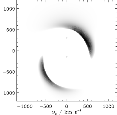
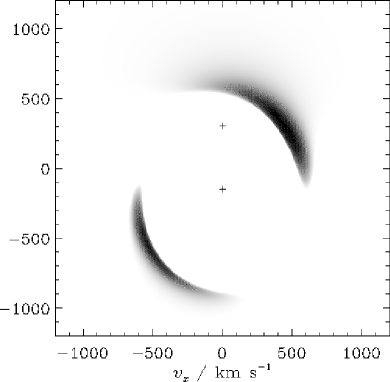
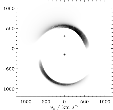
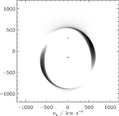
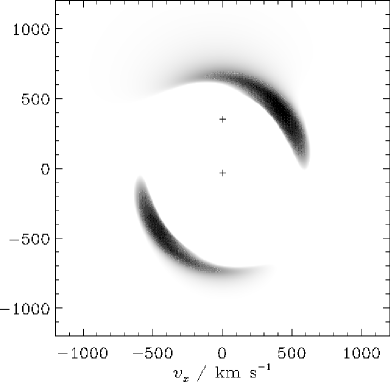
Figure 3: Simple synthetic tomograms for a disc in a binary. The velocity scale is based on the orbital parameters of IP Peg. The plotted intensity is proportional to the elevation of the disc above its undistorted value. Top left: standard parameters, as in Fig. 2. Top right: standard except that $\alpha=0.3$. Middle left: standard except that ${\rm We}=0.1$. Middle right: standard except that ${\rm We}=1$. Bottom left: standard except that $\gamma=1.2$. Bottom right: standard except that $q=0.1$ (the velocity scale assumes the same value of $GM_{1}/a$ as in IP Peg).

6.3 Emission lines and synthetic Doppler tomograms

This suggests that the observed patterns can be explained if the line emission is correlated with the thickness of the disc rather than the continuum brightness. This is consistent with the notion that the emission lines originate in parts of the disc that are elevated and therefore irradiated from the centre of the system by the white dwarf, boundary layer and/or inner disc (Robinson et al. 1993).

Simple synthetic Doppler tomograms based on this premise can then be constructed by plotting an image representing the excess elevation of the disc in velocity space. The quantity plotted in Fig. 3 is $f_{H}-f_{H0}$, where

$$f_{H0}=\left(1+{{9}\over{4}}{\rm We}\,\alpha\right)^{13/28}$$ (121)

is the constant value of $f_{H}$ in the absence of star 2. The velocity field used in constructing the tomograms is the orbital motion of Paczyński’s orbits, translated into the inertial frame.

These synthetic tomograms should not be considered as a serious attempt to reconstruct the observed data, such as that made by Steeghs & Stehle (1999). This would require a better understanding of the mechanism of line emission and a proper treatment of the instrumental and data-analytical limitations of Doppler tomography. Rather, Fig. 3 should be taken as an indication of the probable locations in velocity space of line emission under the irradiation hypothesis.

The dependence of the two-armed patterns on the disc parameters is rather subtle. Increasing the values of $\alpha$, $\alpha_{\rm b}$ or ${\rm We}$ can cause phase shifts that rotate the patterns to some extent. Decreasing $\gamma$ moves the vertical resonance outwards in real space (inwards in velocity space) and can also increase the amplitude of the distortion by making the disc more compressible.

6.4 The role of the vertical resonance

The significance of the vertical resonance in this problem can be demonstrated by considering an approximate model that corresponds to a linear, inviscid analysis of the full equations. In the limit $\alpha,\alpha_{\rm b}\to 0$ the dimensionless turbulent stress coefficients $t^{ab}$ tend to zero and one obtains the much simpler system of ODEs

$$g_{\Omega}\left(-\partial_{\phi}\ln f_{1}+{{13}\over{2}}\partial_{\phi}\ln f_{2}\right)=-14f_{3}-3g_{1},$$ (122)

$$g_{\Omega}\left({{1}\over{\gamma-1}}\right)\partial_{\phi}\ln f_{2}=-\left({{\gamma+1}\over{\gamma-1}}\right)f_{3}-g_{1},$$ (123)

$$g_{\Omega}\partial_{\phi}f_{3}=-f_{3}^{2}-g_{5}+f_{2}.$$ (124)

When the tidal distortion is weak, one may write $f_{2}=1+\delta f_{2}$, $g_{\Omega}=(1-g_{\omega})+\delta g_{\Omega}$ and $g_{5}=1+\delta g_{5}$, where $\delta f_{2}$, $f_{3}$, $\delta g_{\Omega}$, $g_{1}$ and $\delta g_{5}$ are small quantities. In the linear approximation, products of small quantities may be neglected, and this leads to a linear, inhomogeneous equation of second order for $\delta f_{2}$,

$$\left[(1-g_{\omega})^{2}\partial_{\phi}^{2}+(\gamma+1)\right]\delta f_{2}=X,$$ (125)

where

$$X=(\gamma+1)\delta g_{5}-(\gamma-1)(1-g_{\omega})\partial_{\phi}\delta g_{1}.$$ (126)

The forcing function may be resolved into Fourier components,

$$X(\phi;\lambda)={\rm Re}\sum_{m=0}^{\infty}X_{m}(\lambda)\,{\rm e}^{{\rm i}m\phi},$$ (127)

where the coefficients $X_{m}$ are real by virtue of the symmetry of Paczyński’s orbits. The solution is then

$$\delta f_{2}={\rm Re}\sum_{m=0}^{\infty}\left[(\gamma+1)-m^{2}(1-g_{\omega})^{2}\right]^{-1}X_{m}\,{\rm e}^{{\rm i}m\phi}.$$ (128)

It is singular at the vertical resonances, where the quantity in square brackets vanishes. Now

$$g_{\omega}=(1+q)^{1/2}\left({{\lambda}\over{a}}\right)^{3/2},$$ (129)

and so the inner/outer resonance for mode $m>0$ occurs at

$${{\lambda}\over{a}}=(1+q)^{-1/3}\left[1\mp{{1}\over{m}}(\gamma+1)^{1/2}\right]^{2/3},$$ (130)

as determined by Lubow (1981). In particular, for $q=0.5$ and $\gamma=5/3$, the $m=2$ inner vertical resonance occurs at $\lambda/a\approx 0.282$.

The phase of the response to $m=2$ forcing changes by $\pi$ as one passes through the radius of the resonance. In the linear, inviscid limit, the response is formally singular at the resonance. In reality, the response is limited by the emission of a wave (Lubow 1981), or by non-linearity or dissipation (Ogilvie, in preparation). The singularity is then avoided and a smooth variation of amplitude and phase occurs.

The distortion of the thickness of the disc is sensitive mainly to the quantity $f_{2}$, according to equation (120). Therefore the vertical distortion is amplified in the vicinity of the vertical resonance and undergoes a phase shift as one passes through the resonance. This effect can be seen in Fig. 2 (right panel). For the $m=2$ component of the solution, the phase shift of $\pi$ corresponds to a rotation of the peak through $90\degr$. This lends a certain ‘spirality’ to the pattern in the vicinity of the resonance. However, the solution does not represent a wave or shock, and the shape of the pattern is independent of the thickness of the disc.

7 Summary and discussion

In this paper I have constructed a detailed semi-analytical model of the non-linear tidal distortion of a thin, three-dimensional accretion disc by a binary companion on a circular orbit. The analysis allows for vertical motion and radiative energy transport, and introduces a simple model for the turbulent magnetic stress. The fluid dynamical equations are solved by means of a consistent asymptotic expansion, using the fact that the disc is thin. The solution is formally exact in the limit of a thin disc.

The tidal distortion affects quantities such as the surface brightness of the disc and its thickness. As expected, the distortion is greatest in the outer part of the disc and is predominantly two-armed. An important feature of the solution is the $m=2$ inner vertical resonance, first analysed by Lubow (1981), which typically lies within the tidal truncation radius in binary stars. This intrinsically three-dimensional effect has a significant influence on the amplitude and phase of the tidal distortion.

I have shown that the two-armed features observed in Doppler tomograms of the discs of dwarf novae in outburst find a natural explanation if the emission is associated with the tidally thickened sectors of the outer disc that are elevated and may therefore be irradiated by the white dwarf, boundary layer and/or inner disc during the outburst. There is a slight spirality to the structure, arising from the phase shift that occurs on passing through the vertical resonance. There is some dependence of the pattern on the mass ratio and the dimensionless parameters $(\alpha,\alpha_{\rm b},{\rm We},\gamma)$ of the disc (defined in Section 4). In particular, the adiabatic exponent $\gamma$ determines the location of the vertical resonance. Future observations of higher quality might help to constrain the values of these parameters. In principle, the distortion of the continuum surface brightness of the disc, which displays a different pattern (e.g. Fig. 2), might also be seen in eclipse-mapping observations.

This possible interpretation of the observed features is fundamentally different from one based on spiral waves or shocks. There are no waves or shocks in the present analysis. The pattern of emission merely reflects the tidal distortion of the disc and is independent of the angular semi-thickness $H/r$, in the limit that this is small. The observability of the pattern will nevertheless vary during the outburst cycle depending on the spreading of mass to the outer parts of the disc and, in the irradiation hypothesis, on the luminosity of the central regions.

In a recent paper, Smak (2001) has presented arguments against the interpretation of the observed features as spiral shocks. He argues in favour of the irradiation hypothesis and suggests that sectors of the outer disc may be elevated through the horizontal convergence of the three-body orbits. The present paper supports the arguments of Smak (2001) to a certain extent, but within the context of a three-dimensional fluid dynamical model. The principal factors leading to the thickening of the disc can be seen in Section 6.4. Vertical expansions and contractions are driven by the variation of the vertical gravitational acceleration around the tidally distorted orbits and, to some extent, by the horizontal convergence of the flow in the binary plane. The response of the disc to this forcing is regulated by the inner vertical resonance.

The analysis in this paper could be extended and improved in a number of ways. Mass input to the disc, its ultimate tidal truncation, and the spreading of mass during an outburst, should properly be discussed within the context of the evolutionary equation for the surface density, alluded to in Section 5.3 but not derived here. The solution of this equation would determine the relative weighting to be assigned to the different orbits. The viscoelastic model for the turbulent stress, although an improvement on purely viscous treatments, could also be refined. Finally, a better understanding of the mechanism of line emission would enable a closer connection to be made between the computed models and the observational data.

References

- [] Balbus S. A., Hawley J. F., 1998, Rev. Mod. Phys., 70, 1
- [] Bate M. R., Ogilvie G. I., Lubow S. H., Pringle J. E., 2001, MNRAS, submitted
- [] Godon P., Livio M., Lubow S. H., 1998, MNRAS, 295, L11
- [] Goldreich P., Tremaine S., 1979, ApJ, 233, 857
- [] Groot P. J., 2001, ApJ, 551, L89
- [] Hirose M., Osaki Y., 1990, PASJ, 42, 135
- [] Joergens V., Spruit H. C., Rutten R. G. M., 2000, A&A, 356, 33
- [] Larson R. B., 1990, MNRAS, 243, 588
- [] Lin D. N. C., Papaloizou J. C. B., 1986, ApJ, 307, 395
- [] Lin D. N. C., Papaloizou J. C. B., 1993, in Levy E. H., Lunine J., eds, Protostars and Planets III, Univ. Arizona Press, Tucson, p. 749
- [] Lubow S. H., Shu F. H., 1975, ApJ, 198, 383
- [] Lubow S. H., 1981, ApJ, 245, 274
- [] Lubow S. H., 1991, ApJ, 381, 259
- [] Lubow S. H., Ogilvie G. I., 1998, ApJ, 504, 983
- [] Lubow S. H., Pringle J. E., 1993, ApJ, 409, 360
- [] Ogilvie G. I., 1998, MNRAS, 297, 291
- [] Ogilvie G. I., 1999, MNRAS, 304, 557
- [] Ogilvie G. I., 2000, MNRAS, 317, 607
- [] Ogilvie G. I., 2001, MNRAS, 325, 231
- [] Paczyński B., 1977, ApJ, 216, 822
- [] Papaloizou J. C. B., Pringle J. E., 1977, MNRAS, 181, 441
- [] Robinson E. L., Marsh T. R., Smak J. I., 1993, in Wheeler J. C., ed., Accretion Disks in Compact Stellar Systems, World Scientific, Singapore, p. 75
- [] Savonije G. J., Papaloizou J. C. B., Lin D. N. C., 1994, MNRAS, 268, 13
- [] Sawada K., Matsuda T., Hachisu I., 1986, MNRAS, 219, 75
- [] Shu F. H., Cuzzi J. N., Lissauer J. J., 1983, Icarus, 53, 185
- [] Smak J. I., 2001, Acta Astron., 51, 295
- [] Spruit H. C., 1987, A&A, 184, 173
- [] Steeghs D., Harlaftis E. T., Horne K., 1997, MNRAS, 290, 28
- [] Steeghs D., Stehle R., 1999, MNRAS, 307, 99
- [] Steeghs D., 2001, astro-ph/0012353
- [] Stehle R., Spruit H. C., 1999, MNRAS, 304, 674
- [] Szébehely V. G., 1967, Theory of Orbits, Academic Press, New York