Boundary Corrections in Fractal Analysis of Galaxy Surveys

Abstract

The analysis of redshift surveys with fractal tools requires one to apply some form of statistical correction for galaxies lying near the geometric boundary of the sample. In this paper we compare three different methods of performing such a correction upon estimates of the correlation integral in order to assess the extent to which estimates may be biased by boundary terms. We apply the corrections illustrative examples, including a simple fractal set (Lévy flight), a random $\beta$-model, and a subset of the CfA2 Southern Cap survey. This study shows that the new “angular” correction method we present is more generally applicable than the other methods used to date: the conventional “capacity” correction imposes a bias towards homogeneity, and the “deflation” method discards large-scale information, and consequently reduces the statistical usefulness of data sets. The “angular” correction method is effective at recovering true fractal dimensions, although the extent to which boundary corrections are important depends on the form of fractal distribution assumed as well as the details of the survey geometry. We also show that the CfA2 Southern sample does not show any real evidence of a transition to homogeneity. We then revisit the IRAS PSCz survey and “mock” PSCz catalogues made using N-body simulations of two different cosmologies. The results we obtain from the PSCz survey are not significantly affected by the form of boundary correction used, confirming that the transition from fractal to homogeneous behaviour reported by Pan & Coles (2000) is real.

1 Introduction

There has been considerable controversy over a long period about whether the distribution of galaxies in the Universe is homogeneous on large scales, or whether structure might persist indefinitely in the manner of fractal (e.g. Coleman & Pietronero 1992, hereafter CP92; Peebles 1993). This debate revolves around the validity of the Cosmological Principle on scales up to the present observational depth of galaxy surveys. The assumption of homogeneity plays such an important role in cosmology that it is important to establish its validity in the most rigorous possible manner using the most appropriate statistical tools. Instead of the usual two-point correlation function, $\xi(r)$, which assumes homogeneity at the outset, these studies usually exploit a function known as the conditional density, which does not assume that the global mean density of points $\langle n\rangle$ is determined by the sample in question, or even that it exists at all. The global mean density for a fractal set is not a useful concept in any case (Coleman et al 1988; CP92). For non-fractal set for which the mean density is well-defined, the conditional density $\Gamma(r)$ is related to the usual two-point correlation function via

$$\frac{\Gamma(r)}{\langle n\rangle}=1+\xi(r)=g(r).$$ (1)

One of the consequences of a fractal distribution is that the quantity $g(r)$ has a power-law dependency on scale:

$$g(r)\propto r^{D-3},$$ (2)

where $D$ is (loosely) called the fractal dimension; see later for more rigorous definitions. A simple fractal will have a constant value of $D$, whereas a structure that tends towards uniformity will have $D\rightarrow 3$ at some scale.

Some authors have claimed to have found a transition from quasi-fractal behaviour on small scales to a homogeneous behaviour on large scales, with a crossover depth around $30h^{-1}$ Mpc ($h$ is Hubble’s constant in units of 100 km s^-1 Mpc^-1). Examples of data sets analysed this way include the Perseus-Pisces survey (Guzzo et al. 1991), the CfA slice (Lemson & Sanders 1991), the ESO Slice Project (Scaramella et al. 1998) and the Las Campanas redshift Survey (Kurokawa, Morikawa & Mouri 2001). There are other papers in support of homogeneity on large scale, but advocating a different scale at which the transition occurs (Hatton 1999; Bharadwaj, Gupta & Seshadri 1999).

On the other hand, advocates of a purely fractal Universe argue that, up to the presently-observed scales, there is no indication of such a transition at all and that the apparent crossover at $30h^{-1}$ Mpc claim is spurious. Possible causes of this spurious detection are: the use of inappropriate statistical tools, i.e. the two-point correlation $\xi(r)$; errors resulting from uncertainties in the K-correction; misleading boundary corrections; and so on (e.g. CP92; Sylos Labini et al 1996; Joyce et al 1999; Best 2000). In this paper we address the last of these issues, the one which is most often flagged as a possible mechanism for forcing a fractal distribution to display a false signature of homogeneity. Previous papers have examined the behaviour of the conditional density under various forms of boundary correction, with the conclusion is that $g(r)$ and consequently the scale of the crossover are almost independent of such boundary corrections (Lemson & Sanders 1991; Provenzale, Guzzo & Murante 1994). These arguments are largely based on their analysis of CfA and mock data sets.

In this work we examine the effect on the correlation integral (CI), mathematically the integral form of the conditional density mentioned above (Grassberger & Procaccia 1983; Borgani 1995). Boundary corrections appear more explicitly in the CI approach than with the conditional density, which has led to a criticism of this approach (CP92; Marcelo & Alexandre 1998; Sylos Labini et al 1996). However, the only method which is free from any possible effect of boundaries is one in which no correction is used at all (e.g. Pietronero, Montuori & Labini 1997). This inevitably reduces the effective depth of the survey and reduces the number of galaxies. This, in turn, makes it harder to see any transition to homogeneity and reduces the statistical confidence of any analysis method. The motivation for this work is to find a recipe for dealing with boundary effects that offers a reasonable compromise between full use of the catalogues and the possible biases induced by boundary problems, as guide for future analysis of the forthcoming catalogues, such as the 2DF galaxy redshift survey (Colless et al. 2001). It is also important to establish the robustness of the results we obtained in a previous paper for the PSCz (Pan & Coles 2000, hereafter PC) in the light of this comparison.

We will begin in Section 2 with brief description of the CI and discuss the role of boundary corrections in Section 3. In Section 4 we apply the different methods to some illustrative examples. We then, in Section 5, we revisit the PSCz survey studied by PC, alongside mock catalogues made from N-body simulations. The conclusions and a discussion are in Section 6.

2 The Correlation Integral

The measure we use for fractal dimension estimation is constructed from the partition function,

$$Z(q,r)=\frac{1}{N}\sum_{i=1}^{N}p_{i}(r)^{q-1}\propto r^{\tau(q)},$$ (3)

with $p(i)=n_{i}(r)/N$, where $n_{i}(r)$ is the count of objects in the cell of radius $r$ centered upon an object labelled by $i$ (which is not included in the count). For each value of $q$ in equation (3) correponding to relevant moment of the cell-count, one can have a different scaling exponent of the set $\tau(q)$, which induces the so-called Renyi dimensions:

$$D_{q}=\frac{\tau(q)}{q-1}$$ (4)

forming the spectrum of fractal dimensions for a fractal measure on the sample. The terminology applied to a set in which the $D_{q}$ are functions of $q$ is a multifractal. The special case $D_{1}$ for $q=1$ cannot be obtained from equation (3) but should be derived from

$$S(r)=\frac{1}{N}\sum_{i=1}^{N}\log p_{i}(r)\propto r^{D_{1}},$$ (5)

where $S(r)$ is the partition entropy of the measure on the sample set; $D_{1}$ is consequently termed the information dimension (Fedar 1988). The special case $q=2$ leads to the definition of $D_{2}$, described in equation (3). This is the most important exponent in this context and is generally called the correlation dimension. As stated above, it is related to the usual two-point correlation function $\xi(r)$ for a sample displaying large-scale homogeneity (Peebles 1980). If the mean number of neighbours around a given point is $\langle n\rangle$ then

$$\langle n\rangle=4\pi\bar{n}\int_{0}^{r}[1+\xi(s)]s^{2}ds.$$ (6)

In this case $\langle n\rangle\sim r^{\alpha}$ means $\alpha=D_{2}$. A homogeneous distribution has $D_{2}=3$, whereas a power-law in $1+\xi(r)=g(r)\sim r^{-\gamma}$ yields $D_{2}=3-\gamma$.

To account for edge effects and the selection function, we have to weight local count around $i$th object according to

$$n_{i}(r)=\frac{1}{f_{i}(r)}\sum_{j=1}^{N}\frac{\Psi(|\textbf{r}_{j}-\textbf{r}_{i}|-r)}{\phi(r_{j})},$$ (7)

and

$$\Psi(x)=\left\{\begin{array}[]{cc}1,&x\leq 0\\ 0,&x>0\end{array}\right..$$ (8)

For magnitude (or flux) limited sample $\phi(r)$ is exactly the luminuosity selection function, while $\phi(r)=1$ for volume limited sample. It is in the weighting factor $f_{i}(r)$ that the question of appropriate boundary corrections is most important.

3 Boundary Correction Methods

In the literature, there are two standard ways of handling boundary corrections in this type of analysis. The obvious one is the capacity correction which has been used in a series of papers analysing galaxy catalogues (Martínez & Coles 1994; Pan & Coles 2000) and cluster catalogues (Borgani & Martínez et al. 1994). In this prescription, counts for those cells near the boundary are weighted by a factor $f_{i}(r)$ determined by the capacity (for 3-dimensions this is the volume) of the cell with radius $r$ included within the sample space. This is probably the most natural idea how to perform a boundary correction, but it may give rise to artificial homogeneity of the sample, as pointed out for example by CP92. Consider the example of a ball of radius $r$ with points inside it distributed according to a density law $n\propto r^{D}$ with $D<3$. If we extend the cell count around the ball’s centre to scale $R>r$ using the capacity correction, we will be extrapolating the count to scale $R$ with the law of $n\propto r^{3}$. This criticism is made forcefully by those advocating the purely fractal picture.

A radical way to circumvent this problem is to discard any cells not completely contained within the sample space; we name this the deflation method in this paper. The $N$ in equations (3) and (5) is then not the total number of galaxies but the number of those left after elimination. This correction has been used quite often in estimates based on the conditional density (e.g. CP92). The largest scale that can be detected when this method is used is the radius of the biggest sphere that can be entirely fitted into the sample space. This is defined to be the effective sample radius $R_{s}$ and is very much less than the real depth of most samples, especially ‘pencil-beam’ or ’fan’ surveys, or surveys containing ’holes’ due to variations in completeness of sky coverage. This correction greatly cut down the effectiveness of such surveys. Typically, for a sample of depth $\sim 150h^{-1}$ Mpc, the effective depth can be as small as $\sim 20h^{-1}$ Mpc. This is not an efficient use of the data.

A second crucial shortcoming of this approach is that it is statistically unreasonable. As the size of a cell $R$ is increased, the number of cells remaining in the sample decreases until the effective sample radius $R_{s}$ is reached. On large scales, therefore, the correlation integral is usually dominated by a few cells around galaxies with located at particular places within the survey geometry. In the sense of statistics this is rather unfair: the measure $Z(r)$ is averaged over large number of cells on small scales, while very few are included on large scales. This reduces the statistical significance of measured values quite considerably for cells of size similar to the effective radius.

Note also that some authors (e.g. CP92), have used the conditional density about the observer rather than around individual galaxies because of the impossibility of reaching scales larger than $R_{s}$. They have thus inferred the validity of a fractal picture up to about a few hundred Megaparsec. This is highly misleading. First of all, a power-law around one peculiar point is not proof of fractal scaling. The behaviour of $g(r)$ around the observer is a special event and should not be used as a description of general property of the sample. Furthermore, the $g(r)$ is based on the points located almost at the sample’s centre when $r$ is close to $R_{s}$, but in case of $r>R_{s}$, $g(r)$ is based entirely on the observing point. These are not measuring the same thing, so any claimed inhomogeneity based on such an approach begs the question.

Of course any boundary correction has to rely on some assumption about the distribution of points beyond the sample boundary, and to some extent this inevitably leads to a bias of some kind. We have to be aware of what kind of bias this is, and what the statistical consequences are so that we can interpret our results in a reasonable way. The discussion above indicates that the two conventional prescriptions, the capacity and deflation corrections, do not succeed in these aims. We therefore need to find new ways to perform a more suitable edge correction. Any useful new method should make minimal assumptions while making maximal use of the information contained within the sample.

In this spirit, we propose a third correction: the angular correction. This proposal stems from the realisation that the appropriate measure in equation (3) relates to a scaling law that depends only on the radius $r$ and which has nothing to do with the angles. From this point of view, we can construct a correction relying on the solid angular occupation of the sample relative to the cell’s centre, as illustrated in Figure 1. The correction requires two steps, the first of which resembles the capacity correction in fixing the factor $f_{i}(r)$ and the second is similar to the deflation method when counting neighbours. For a point $i$ in the sample, we calculate $4\pi[1-f_{i}(r)]$ as the solid angle subtended at the point in question by intersection of a sphere of radius $r$ with the boundary. Let’s mark the joint space of the cones in the sphere opened by these solid angles $w^{*}$, then correspondingly during neighbour counting process the points belonging to $w^{*}$ are excluded. We can increase $r$ for detection until either one of the correction factors equals zero.

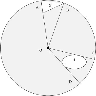
Figure 1: An illustration in two dimensions of the angular correction method to the CI works with a boundary. A cell with radius $r$ is drawn on point $0$ inside the sample. The shaded region is inside the sample; two regions not belonging to the sample space are labelled 1 and 2. The angles opened by them are $\theta_{AOB}$ and $\theta_{COD}$ respectively. The correction factor is then $f_{O}(r)=1-(\theta_{AOB}+\theta_{COD})/2\pi$. And when we count the neighbours, we need to exclude those points in the regions delimited by $AOB$ and $COD$. The application to solid angles in 3D is straightforward as described in the text.

The underlying assumption of this method is of statistical isotropy. The capacity correction relies on homogeneity too, because it incorporates an extra correction to the radial part of the cell count. In this correction, the availability of a sample point depends on its largest distance to a boundary in contrast to the deflation method where it is the smallest scale that counts. This does increase significantly the usable depth of the sample. The maximum scale that can guarantee that all sample points are available, which keeps the measure statistically fair, is the smallest one of the largest distances of these points to the boundary surface.

4 Illustrative Examples

It is hard to show analytically how much these boundary correction methods reflect the true scaling behavior of samples and which one is the best order from the menu of edge corrections. We have instead to turn to numerical tests. Since we are talking about fractal analysis, it will be worthwhile to consider these methods in the context of a simple fractal set with known dimension. After establishing the results of this we can understand their effects on real samples and catalogues from n-body simulation. The form of the sample boundary will itself play a role in determining the importance of boundary corrections. Since these are primarily for illustration of the possible pitfalls, and we can’t in any case simulate every possible boundary of every possible sample, we will proceed using sets with relatively simple boundaries.

4.1 Monofractal set: the random Lévy flight

Let us just start with a monofractal sample with dimension $D$, which is obtained by the simple Lévy flight (Meakin 1998). In this case, the $D$ coincides with the correlation dimension $D_{2}$. The Lévy flight is one species of fractal Brownian random walk with variable step size $X$, such that the probability of $X$ exceeding a particular value $x$ satisfies

$$P(X\geq x/x_{0})=\left\{\begin{array}[]{cc}(x/x_{0})^{-D},&x/x_{0}>1\\ 1,&x/x_{0}\leq 1\end{array}\right.,$$ (9)

which leads to a fractal point set of dimension $D$ on scales $X\gg 1$ (Mandelbrot, 1977). The parameter $x_{0}$ here plays the role as the minimum step size of the random walk.

We construct a cube-shaped sample of $D=1.2$, roughly that observed in galaxy clustering. We use a test volume of $60\times 60\times 60$ Mpc, and set up the minimum step size $x_{0}=0.2$ Mpc. The correlation integrals obtained using the different edge treatments discussed in Section 3 are shown in Figure 2 and the dimensions obtained in different domains are listed in Table 1. Because we set the minimum step size of the Lévy walk to be $0.2$ Mpc, it is not surprising that the correlation integrals below $\sim 1$ Mpc, where they are dominated by discreteness, are quite steep. When $r\gg x_{0}$, the capacity correction obviously contaminates the estimation badly. Larger and larger values of the dimension are obtained with increasing scale; this trend is entirely spurious. The deflation method provides better answer but the local dimension in this case fluctuates wildly around the true value, which may arise from the fact that what we measure with equation (3) on different scales is effectively coming from a different point set. The performance of angular correction is promisingly steady and it accurately recovers the true dimension, which encourages our conjecture that this one is superior to the others.

Lévy Flight	Capacity	Angular	Deflation
$D_{2}\begin{array}[]{c}1\sim 10\,{\rm Mpc}\\ >10\,{\rm Mpc}\end{array}$	$\begin{array}[]{c}1.33(1)\\ 1.84(3)\end{array}$	$\begin{array}[]{c}1.18(1)\\ 1.19(3)\end{array}$	$\begin{array}[]{c}1.17(4)\\ 1.01(8)\end{array}$
$r_{\rm max}({\rm Mpc})$	—	$41.2$	$30$

Table 1: Correlation dimensions $D_{2}$ for different scale ranges of the Lévy flight generated sample with $D=1.2$. Errors are from goodness-of-fit considerations only. $r_{\rm max}$ indicates the largest available scale as discussed in text for angular correction and deflation method.

Figure 2: The correlation integral analysis under three different boundary correction methods for Lévy flight generated fractal point set with dimension $D=1.2$ and minimum step size $x_{0}=0.2$ Mpc. The sample space is a $60\times 60\times 60$ Mpc cube. In this plot and all the plots hereafter, the value of $h$ is set to be unity. Panel (a) shows the correlation integrals $Z(q=2)$ of equation (3), the straight line of slope $D=1.2$ is plotted as reference. Panel (b) displays the local correlation dimensions against scale by fitting every five consecutive points. The excess dimension excess below $\sim 1$ Mpc is a resolution effect. It is very clearly seen that the capacity correction can seriously mask the true scaling properties. The angular-corrected estimation is superior in providing quite stable and accurate results to the one corrected by deflation method. The maximum available scales for the deflation method and angular correction are $30$ Mpc and $\sim 40$ Mpc respectively.

This example constitutes a rather severe test because each realisation of the random Lévy flight is highly anisotropic. Although the pattern of large-scale structure does display filaments, they are by no means as exaggerated as this. In the following we look at a less extreme model.

4.2 A different example: The $\beta$-model

We next examine a simple self-similar cascading $\beta$ model. Points are generated by a breaking cascade from the parent cube with size $L_{0}$ into $M$ smaller but similar cubes with size $L_{1}=L_{0}/n$ (usually $n=2$, thus $M=n^{3}$). Each cube is then assigned a survival probability $p$ until the next iteration at which it stands a chance of breaking again. The final set is the collection of all the survived points (cubes) after $k$ iterations (see Castagnoli & Provenzale 1991). This model is qualitatively similar to hierarchical clustering.

Here the survival probability $p$ remains constant for all cubes and all iterations. The fractal dimension of this simple model is given by

$$D=\lim_{k\rightarrow\infty}\frac{\log(pM)^{k}}{\log n^{k}}=\frac{\log pM}{\log n}.$$ (10)

Figure 3: As Figure 2 (except here arbitrary scale unit is used), but for the $\beta$-model. The parameters chosen are $L_{0}=1000$ and $p=0.4352$ corresponding to $D=1.8$. About 20,000 points are generated for this analysis. The differences between capacity and angular correction are not so dramatic as the Lévy flight example, but we can still identify the systematic increase of local dimensions under capacity correction.

$\beta$ model	Capacity	Angular	Deflation
$D_{2}\begin{array}[]{c}<100\\ >100\end{array}$	$\begin{array}[]{c}1.86(1)\\ 2.09(1)\end{array}$	$\begin{array}[]{c}1.85(1)\\ 1.92(2)\end{array}$	$\begin{array}[]{c}1.84(1)\\ 1.83(4)\end{array}$
$r_{\rm max}$	—	$870$	$340$

Table 2: Correlation dimensions $D_{2}$ for different scale ranges of the $\beta$ model with $D=1.8$. Errors are from goodness-of-fit considerations only. The quantity $r_{\rm max}$ is the largest available scale as discussed in text for angular correction and deflation method.

We produced the sample using $p=0.4352$ and $n=2$ correponding to $D=1.8$. The parent cube which also defines our sample space is of size $L_{0}=1000$. About 20,000 points are generated for our analysis. The results are displayed in Figure 3 & Table 2. Panel (b) of Figure 3 shows that differences in the three methods arise at a scale of $\sim 100$. Below that, unlike the highly anisotropic Lévy flight example, boundary corrections have little effects. Angular correction agrees with capacity correction out to a scale of a few hundred, but angular correction does not introduce an apparent trend to higher dimensions on scales larger than $\sim 100$, which capacity correction does.

Although in this case the differences between the three methods are somewhat less extreme, it is still the case that the angular correction method is close to the correct answer, while the capacity correction produces an artificial tendency towards homogeneity.

4.3 CfA2-South Survey

The two toy examples we have displayed illustrate that one should take care in implementing boundary corrections that may influence the measured fractal properties of the sample. We now turn to a real sample, although by now it is of historical importance only. The example we choose is the well-studied CfA2-South galaxy survey (Huchra et al. 1999). Previous research has indicated its dimension $D=1.8\sim 2.0$ up to $\sim 30h^{-1}$ Mpc approached with different fractal tools (Joyce, Montuori & Sylos Labini 1999; Kurokawa, Morikawa & Mouri 1999). The question we ask is whether, given the potential dangers we described above, there is evidence that this survey displays a tendency towards homogeneity?

The sample we study covers $20^{h}\leq\alpha\leq 4^{h}$ in right ascension and $-2.5^{\circ}\leq\delta\leq 90^{\circ}$ in declination, containing 4390 galaxies in total with magnitude $m_{B(0)}\leq 15.5$. Following Park et al. (1994), we exclude areas where there is significant interstellar extinction from our Galaxy: $20^{h}\leq\alpha\leq 21^{h}$; $3^{h}\leq\alpha\leq 4^{h}$; $21^{h}\leq\alpha\leq 2^{h}$ and $b>-25^{\circ}$; $2^{h}\leq\alpha\leq 3^{h}$ and $b>-45^{\circ}$. Here $b$ is the Galactic latitude. The distances are computed from the redshift $z$ using the Mattig formula,

$$r=\frac{c}{H_{0}{q_{0}}^{2}(1+z)}[q_{0}z+(q_{0}-1)\cdot(\sqrt{2q_{0}z+1}-1)]\,,$$ (11)

with $H_{0}=100h^{-1}$ km s^-1 Mpc^-1 and $q_{0}=0.5$.

We construct a volume-limited sample with magnitude threshold $M_{B(0)}=-18.46$. The absolute magnitude is obtaineed from

$$M_{B(0)}=m_{B(0)}-5\log[r(1+z)]-25-Kz\,,$$ (12)

where the $K$-correction factor $K$ here is taken to be $3$ (Park et al 1994). The sample thus has 766 galaxies, and its depth is $60h^{-1}$ Mpc corresponding to a redshift $z=0.02$.

Figure 4: Correlation integrals of CfA2-South volume-limited sample from different boundary corrections. The sample size is $60h^{-1}$ Mpc, the minimum and maximum separation between galaxies are $0.03h^{-1}$ Mpc and $76h^{-1}$ Mpc. As in Fig. 2, panel (a) shows the measure $Z$; and panel (b) gives the local $D_{2}$, in which the points from the capacity correction are connected with a line which shows larger dimensions than the other two different methods, and also the results from Joyce et al (1999).

CfA2-South	Capacity	Angular	Deflation
$D_{2}$	$2.07(3)^{*}$	$1.84(2)$	$1.83(2)$
$r_{\rm max}(\rm Mpc)$	—	$\sim 43$	$\sim 11$

^∗ If we fit it above $10h^{-1}$ Mpc, $D_{2}=2.54\pm 0.03$.

Table 3: Correlation analysis of CfA2-South sample. $D_{2}$ is gained via linear regression of $\log(Z)$ vs $\log(r)$ in full detected scale range. As before, $r_{\rm max}$ is the maximum scale.

Our calculations are illustrated in Figure 4 and Table 3. The results are quite consistent with the analysis of Joyce et al (1999). They demonstrate the fractal nature of the CfA2-South galaxy survey sample, with $D_{2}\sim 1.8$ but with a scale extending to $\sim 40h^{-1}$ Mpc with our new angular correction rather than the largest $R_{s}\approx 30h^{-1}$ Mpc obtained from the volume-limited sample VL205 (with limiting absolute magnitude $M_{B(0)}=-20.5$) using the deflation method.

On small scales, less than $\sim 10h^{-1}$ Mpc, there is little difference among the measures obtained after correction by different methods. This can be easily understood because in this case only a very small number of points needs correction. On larger scales it becomes apparent that the capacity correction produces a trend leading to a homogeneous dimension, similar to the result of Lévy flight. Again, the deflation method and angular correction present behavior consistent with each other. Although the capacity correction does not deviate seriously from the dimension obtained by fitting over the whole range of scales in this case, it definitely disguises the behaviour of the sample with an inclination towards homogeneity (Table 3). It is not clear what is happening with the deflation and angular corrected measures on large scales, but similar fluctuations have already been shown in the Lévy flight simulations (panel (b) in Figure 2). At least there is no tendency to introduce artificial homogeneity, and we see that angular correction demonstrates a more stable measure, i.e. with smaller fluctuations than the deflation method.

4.4 Comments

At this point we can already form a couple of preliminary conclusions about this case and that of the toy fractal sets. First, it is clear that the capacity correction is, in general, not the most appropriate available for fractal analysis. The improper imposition of boundary corrections can substantially confuse the issue of whether a given sample reaches homogeneity or not. On the other hand, our new angular correction behaves well in recovering the true scaling law, with less fluctuations, more effective use of the sample, and a higher level of reliability than the deflation method.

5 The PSCz Survey Revisited

In a previous paper (PC), we analyzed the IRAS infrared galaxy redshift catalogue known as the PSCz survey, with was analyzed with correlation integral using the conventional capacity correction. In that paper it is claimed that the correlation dimension $D_{2}$ above $30h^{-1}$ Mpc is very close to 3 but it still has a value as small as $2.16$ under $10h^{-1}$ Mpc. This argues for a transition from fractal to homogeneity within the range $\sim 10$ to $\sim 30h^{-1}$ Mpc. As we have seen in Section 4, this scale range is very close to the range where the capacity correction begins to effect the true scaling properties of fractal distributions. The question then arises whether the transition phenomenon observed by PC in the PSCz may only be an artifact of the use, in that paper, of the capacity correction. Does the transition to homogenity still appear if we use different boundary corrections?

5.1 Application to the PSCz

A problem of dealing with real samples like this can be their complicated geometrical shape. The PSCz sample, for instance, has troublesome irregular masks (Saunders et al 2000). In particular, the blank strip running across the sky along a longitude line makes it difficult to apply the angular correction directly to the CI measure. Given this difficulty, the correction factors from capacity and angular corrections are estimated via Monte Carlo simulation. We generate sufficient uniformly-distributed points within each cell at a specific scale and simply count how many lie within the sample space. However, the angular correction is still fairly tricky even within this approach. In this case the Monte Carlo simulation does not only involve approximating the edge-correction factors. Neighbour counting is also problematic if the sample space does not have a simply-connected convex geometry, such as if there are holes or cuts in it. These factors dramatically increase the time of computation needed to apply the boundary corrections.

In order to keep the calculations within a manageable bound, we therefore used a subsample of the data used in PC, located in the north galactic hemisphere for the purpose of comparing different boundary correction methods. The other selection criteria are kept as in PC except for the following, latitude $b>30^{\circ}$, longitude $l<120^{\circ}$ or $l>300^{\circ}$ and the distance to the galctic equator plane $r\sin b>10h^{-1}$ Mpc. This subsample contains 1941 galaxies and has convex boundary surface.

Figure 5: Application of the method to the PSCz subsample. The left panel shows $Z(q=2)$ under the different boundary corrections. Two reference lines with $D_{2}=2.30$ and $D_{2}=3.0$ are fitted in regions $r<10$ Mpc and $r>30$ Mpc. The local $D_{2}$ are obtained by fitting 5 consecutive points in the right panel; the results from the capacity correction are connected with a line.

PSCz	Capacity	Angular	Deflation
$D_{2}$ $\begin{array}[]{c}<10\,{\rm Mpc}\\ 10\sim 30\,{\rm Mpc}\\ >30\,{\rm Mpc}\end{array}$	$\begin{array}[]{c}2.31(4)\\ 2.57(3)\\ 2.99(1)\end{array}$	$\begin{array}[]{c}2.32(4)\\ 2.57(3)\\ 2.94(3)\end{array}$	$\begin{array}[]{c}2.34(4)\\ 2.57(3)\\ 3.06(4)\end{array}$
$r_{\rm max}({\rm Mpc})$	—	$\sim 344$	$\sim 104$

Table 4: The correlation dimension$D_{2}$ for different scales of the PSCz subsample under three boundary correction methods and the correponding largest scale explorable. Errors are from goodness-of-fit considerations only.

The results are shown in Figure 5. The mean separation between galaxies in this subsample is $\sim 2.6h^{-1}$ Mpc. Below this scale there is no proper scaling law. The correlation dimensions obtained for different zones above it are listed in Table 4. It is a surprise that none of the boundary correction methods affects either the measure or the estimation of dimensions significantly. On small scales, it is expected that only a very small fraction of galaxies is near the sample edge so that the boundary correction does not have any important influence. On large scales we have already known from analysis of the previous two samples that the capacity correction can bias the measure seriously, but this does not seem to produce a big effect here. The results corrected in different ways are almost the same until the scale reaches $\sim 30h^{-1}$ Mpc, where the local dimension curves begin to diverge. Even at this separation the results appear to fluctuate only around the the homogeneous dimension $D_{2}=3$. This can only be explained as the intrinsic distribution is statistically homogeneous above $30h^{-1}$ Mpc; any boundary correction will then be unable to deflect the result away from the expected $D_{2}=3$ except for chance statistical fluctuations.

The value of $D_{2}$ for $r<10h^{-1}$ Mpc is larger than that given in PC, $D_{2}=2.15$, but close to the value deduced from QDOT (Martínez & Coles 1994), $D_{2}=2.25$. The difference between these three samples is the number of galaxies. There are 1561 galaxies in the QDOT sample, similar to the sample studied here. This discrepancy may be an example of the finite size effect discussed by Sylos Labini et al (1996), or it could be due to redshift-space distortions, but the transition from fractal to homogeneity is still very clear. In order to confirm this, we applied the deflation method to the original sample used in PC; this gives $D_{2}(r>30h^{-1}\,{\rm Mpc})=2.98\pm 0.01$.

Now we can say with confidence the conclusion in PC that there is transition from fractal to homogeneous on scales around $30h^{-1}$ Mpc in this PSCz survey even though PC did not use the safest method of boundary correction.

5.2 Mock PSCz catalogues

Although we have found that analysis of the PSCz sample does not greatly suffer from boundary correction errors, we still need to check the validity of our inferences for samples which do display a mixture of scaling properties, particularly having a gradual transition to homogeneity. The best choice is to deal with mock PSCz catalogues from N-body simulation of cosmological models. This is in any case an interesting exercise, because it may show us how well the n-body simulations mimic real clustering when judged in the light of a statistical approach that differs from the more standard correlation functions and power spectra.

We have studied two different mock PSCz catalogues. The catalogue from SCDM simulates universe with $\Omega_{M}=1$ and shape parameter $\Gamma=0.5$ normalized with COBE data. The other one from $\Lambda$CDM set up $\Omega_{\Lambda}=0.7$, $\Omega_{M}=0.3$ and $\Gamma=0.25$. The details of simulation are described in Cole et al (1998). Both samples are $170$ Mpc deep , include about same number of points as PSCz and their correlation functions are also fitted to agree with PSCz. In order to minimize the effects of differing geometry, we don’t use the the whole data; subsamples are formed exactly in the way we construct the PSCz subsample (except for the depth).

The results are reproduced in Figure 6 & Table 5 and Figure 7 & Table 6 repectively for SCDM and $\Lambda$CDM mock data. Neither simulations shows a sign of significant difference among the three methods for edge correction. The correlation integral delimits the transition to homogeneity perfectly.

What is interesting is on small scales, up to $10$ Mpc, both mock data sets have stronger clustering than the real PSCz survey. The points numbers of the two mock data samples are quite close to the real sample, so this over-clustering should not be interpreted as finite size or discretness. More likely it is due to the difficulty of finding a prescription for identifying galaxies in simulations that follow only the evolution of dark matter. One aspect of this problem is the well-known one that standard CDM models have too much clustering power on small scales, requiring some form of anti-bias to be invoked to explain the observations.

SCDM	Capacity	Angular	Deflation
$D_{2}$ $\begin{array}[]{c}<5{\rm Mpc}\\ 5\sim 30{\rm Mpc}\\ >30{\rm Mpc}\end{array}$	$\begin{array}[]{c}0.97(2)\\ 2.23(6)\\ 2.91(2)\end{array}$	$\begin{array}[]{c}0.96(2)\\ 2.23(6)\\ 2.88(3)\end{array}$	$\begin{array}[]{c}0.98(3)\\ 2.02(6)\\ 2.79(6)\end{array}$
$r_{\rm max}({\rm Mpc})$	—	$\sim 132$	$\sim 54$

Table 5: Correlation dimensions $D_{2}$ and for different scales of the SCDM mock PSCz subsample and $r_{\rm max}$ for angular correction and deflation method. Errors are from goodness-of-fit considerations only.

Figure 6: Fractal analysis of subset of mock PSCz catalogue from n-body simulation of SCDM model. The sample contains 1835 points.

Figure 7: Results of subset of mock PSCz catalogue from $\Lambda$CDM model. This set includes 1751 points.

$\Lambda$CDM	Capacity	Angular	Deflation
$D_{2}$ $\begin{array}[]{c}<5{\rm Mpc}\\ 5\sim 30{\rm Mpc}\\ >30{\rm Mpc}\end{array}$	$\begin{array}[]{c}1.11(1)\\ 2.11(6)\\ 3.00(1)\end{array}$	$\begin{array}[]{c}1.08(1)\\ 2.12(6)\\ 3.04(3)\end{array}$	$\begin{array}[]{c}1.05(2)\\ 2.28(5)\\ 2.92(6)\end{array}$
$r_{\rm max}({\rm Mpc})$	—	$\sim 132$	$\sim 47$

Table 6: Correlation dimensions $D_{2}$ and for different scales of the $\Lambda$CDM mock PSCz subsample and $r_{\rm max}$ for angular correction and deflation methods. Errors are from goodness-of-fit considerations only.

6 Conclusion and Discussion

We have investigated the treatment of edge effects for the fractal analysis based on the correlation integral (CI) for various samples. Generally speaking, on small scales, the CI is almost unaffected by boundary correction just because there are only a few points in the vicinity of boundaries. Finite size and discreteness effects can blur the real dimension on very small scales, however. The proper scaling law has to be sought on scales above some critical scale $r_{0}$ to avoid this problem. Determining the scale that one needs to reach is not trivial. It has been argued on the basis of a Voronoi (1908) model that this scale needs to be about an order of magnitude larger than the Voronoi tesselation radius $r_{v}\sim V_{v}^{1/3}$ in such a model (Sylos Labini et al. 1996), where $V_{v}$ is the Voronoi volume and $r_{v}$ is of order of the mean separation between the Voronoi nuclei. However, the more relevant criterion for the analysis of very deep samples like PSCz is that one simply has to have enough galaxies in the sample to get reliable statistical estimates of the correlation dimension.

On sufficiently large scales, different boundary corrections lead to differences in estimates of statistics extracted from the CI. The capacity correction can introduce extra homogeneity into the CI, while the deflation method reduces the number of available points and can consequently generate big fluctuations and lower statistical significance in the CI. The angular correction leads to a reasonable compromise between the two former effects, although it is difficult to apply it to real samples if they have a complicated geometry, especially if there are holes inside. However in practice the uncertainties introduced by boundary effects depend on the properties of samples under analysis. In a pure fractal set or sample not reaching the homogeneity scale, capacity correction can fool people into thinking that the transition to homogeneity has been observed. In samples whose size extends beyond the transition scale like the PSCz mock catalogues, boundary corrections have only a trivial importance in the analysis. This is a similar conclusion to that reached by Lemson & Sanders (1991) and Provenzale, Guzzo & Murante (1994), although they used the conditional density $g(r)$ rather than the CI which we discuss here.

Whatever the case, it is clear that the capacity correction is not the most suitable for exploring the scaling laws for clustering displayed by galaxy samples. The angular correction we propose has less bias and produces less fluctuations than the others. Of course the relative merits of the different approaches depend on the precise details of survey shape and sampling properties. In general one should establish the reliability of a given result by examining the range of methods. Even the deflation method, though not optimal, can still be used as auxiliary method to get an idea of uncertainties or fluctuations.

Our analysis of CfA2-South sample shows that it is indeed fractal, with dimension $\sim 1.8$ up to $40h^{-1}$ Mpc; there is no sign of tendency toward a homogeneous distribution in this data set. It is known that infrared galaxies distribute more homogeneously than galaxies selected via their luminosity in the optical band. Infrared galaxies are less likely to be found in the inner parts of rich clusters, for example. This may account for the contradiction between the two samples. We can nevertheless expect that the completion of the next generation of large-scale redshift surveys, will establish a transition to homogeneity with a scale somewhere around $30h^{-1}$ Mpc.

The application to subsamples of the PSCz survey indicates that the features of the distribution of infrared galaxies above scale $\sim 30h^{-1}$ Mpc are not modified by any reasonable boundary correction, which in turn provides further supporting evidence for a Universe which is homogeneous on large scales. It remains difficult to put strict error bars on the results, but we can use the values generated by three treatments to get an idea of the errors. This constrains the dimension $D_{2}$ to lie in the range $2.94\sim 3.06$ on large scales, assuring the validity of the results in PC. The QDOT survey is one subset of the present PSCz catalogue, thus the analysis of it by Martínez & Coles (1994) are also supported. Moreover, the observed data behave in precisely the same manner as the simulation results which are based on cosmologies in which the Cosmological Principle applies. However, this satisfying confirmation may not extend to other samples that have produces claims of large-scale homogeneity. For example, we have strong reason to suspect that the claimed tendency-to-homogeneity of the cluster samples from Abell and ACO catalogues by Borgani & Martínez (1994) may not be real, and the distribution of these clusters remains somewhat uncertain, owing to the use of the capacity correction in that study. The difference between angular and capacity dimensions is much smaller when the conditional density is used.

References

- [1] Beacom J.F., Dominik K.G., Melott A.L., 1991, ApJ, 372, 351
- [2] Best J.S., 2000, ApJ, 541, 519
- [3] Bharadwaj S., Gupta A.K., Seshadri T.R., 1999, A&A, 351, 405
- [4] Borgani S., 1995, Phys. Rep. 251, 1
- [5] Borgani S., Martínez V.J., Pérez M.A., Valdarnini R., 1994, ApJ, 435, 37
- [6] Castagnoli C., Provenzale A., 1991, A&A, 246, 634
- [7] Cole S., Hatton S., Weinberg D.H., Frenk C.S., 1998, MNRAS, 300, 945
- [8] Coleman P.H., Pietronero L., Sanders R.H., 1988, A&A., 200, L32
- [9] Coleman P.H., Pietronero L., 1992, Phys. Rep., 231, 311
- [10] Colless M. et al., 2001, MNRAS, submitted, astro-ph/0106498
- [11] Fedar J., 1988, Fractals, Plenum Press, New York
- [12] Grassberger P., Procaccia I., 1983, Physica 9D, 189
- [13] Guzzo L., Iovino A., Chincarini G., Giovanelli R., Haynes M. P., 1991, ApJ, 382, L5
- [14] Hatton S., 1999, MNRAS, 310, 1128
- [15] Joyce M., Montuori M., Sylos Labini F., 1999, ApJ, 514, L5
- [16] Kurokawa T., Morikawa M., Mouri H., 1999, A&A, 344,1
- [17] Kurokawa T., Morikawa M., Mouri H., 2001, A&A, 370, 358
- [18] Lemson G., Sanders R.H., 1991, MNRAS, 252, 319
- [19] Mandelbrot B.B., 1977, Fractals, Freeeman, San Francisco
- [20] Marcelo B.R., Alexandre Y.M., 1998, Braz. J. Phys., 28, 132 (astro-ph/9803218)
- [21] Martínez V.J., Coles P., 1994, ApJ, 437, 550
- [22] Meakin P., 1998, Fractal, scaling and growth far from equilibrium, Cambridge University Press
- [23] Pan J., Coles P., 2000, MNRAS, 318, L51 (PC)
- [24] Park C., Vogeley M.S., Geller M.J., Huchra J.P., 1994, ApJ, 431, 569
- [25] Peebles P.J.E., 1980, The Large Scale Structure of the Universe. Princeton University Press, Princeton
- [26] Peebles P.J.E., 1993, Principles of Physical Cosmology, Princeton University Press, Princeton
- [27] Pietronero L., Montuori M., Labini F.S., 1997, Critical Dialogues in Cosmology, ed. Turok N., World Scientific, Singapore (astro-ph/9611197)
- [28] Provenzale A., Guzzo L., Murante G., 1994, MNRAS, 266, 555
- [29] Saunders W. et al., 2000, MNRAS, 317, 557
- [30] Sylos Labini F., Gabrielli A., Montuori M., & Pietronero L., 1996, Physica A, 226, 195
- [31] Voronoi J., 1908, Reine Angew. Math., 134, 198