Error analysis of the photometric redshift tecnique

Abstract

We present a calculation of the systematic component of the error budget in the photometric redshift technique. We make use of it to describe a simple technique that allows for the assignation of confidence limits to redshift measurements obtained through photometric methods. We show that our technique, through the calculation of a redshift probability function, gives complete information on the probable redshift of an object and its associated confidence intervals. This information can and must be used in the calculation of any observable quantity which makes use of the redshift.

1 Introduction

One of the most basic operations that need to be performed in Cosmology is the measurement of the redshift of any given object. As is well known, such an operation can be more or less readily fulfilled depending on several factors like the brightness of the object, the available instrumentation, and the analysis technique. Given that advancement in science is always driven by work at the very edge of feasibility, it is not surprising that cosmologists often find themselves trying to measure redshifts from objects that are too faint for even the most advanced spectrographs.

This dearth of photons forces astronomers to try and identify spectral features in noisy spectra. More often than is usually believed this causes mistakes that are not easily noticed. This is because spectroscopic redshift errors are often due to human biases (as when the observer makes a choice to identify a possible emission/absorption line amongst comparable noise peaks; or to assign line identifications based on his/her previous experience or personal preference), and also because often the spectroscopic information is not made available for general scrutiny. The particular case of the Hubble Deep Field [Williams et al. 1996], without doubt the most deeply observed patch of the sky, is palmary: not less than five papers have been published with spectroscopic redshifts of multiple, different HDF objects that have later been retracted as ‘erroneous’; see Fernández-Soto et al. (2001, FS01 from here on) for a complete analysis. The effect of those errors in subsequent papers that made use of the wrong spectroscopic lists is difficult to ascertain. It is not straightforward to find a solution to this problem within the usual techniques, because of the sources of bias listed above.

The use of photometric techniques to measure redshifts was suggested as early as 1962 by Baum [Baum 1962], and other authors (Koo 1981, Butchins 1981, Loh & Spillar 1986) pioneered similar ideas to overcome the difficulties associated to spectroscopy of very faint sources. Photometric redshift techniques boomed in the mid 1990s with the arrival of the Hubble Deep Fields–extremely deep images in which exquisite photometry could be performed on thousands of galaxies, over 90 per cent of which were too faint for any spectrograph available at the time, nowadays, or in the near future. Several groups have perfected different approaches (for example Lanzetta, Yahil, & Fernández-Soto 1996; Gwyn & Hartwick 1996; Sawicki, Lin, & Yee 1997; Wang, Bahcall, & Turner 1998; Fernández-Soto, Lanzetta, & Yahil 1999–hereafter FLY99, Furusawa et al. 2000; Benítez 2000; Yahata et al. 2000–hereafter Y00; Fontana et al. 2000; Massarotti et al. 2001) and nowadays it can be said that photometric redshift techniques are an integral part of the standard cosmological toolbox.

Most cosmologists will concur with the opinion that the photometric techniques are useful because they expand the volume of ‘distance-luminosity’ space where redshifts can be measured–even if the values so measured are somehow ‘less precise’ than the spectroscopic ones, a payback most are willing to accept. We find this very concept (the ‘lack of precision’) very difficult to evaluate. It is uncomfortable for any scientist to talk about the accuracy of a measurement whenever a confidence interval has not been assigned to it, and as has been exposed above, that is precisely the problem with spectroscopy of faint sources.

In a previous paper (FS01) we showed that our particular technique is able to measure redshifts of faint objects with a reliability which is comparable (if not superior) to that of the traditional spectroscopic method. We present in this work a simple method that allows for the calculation of accurate confidence intervals around photometric redshift measurements. The use of these confidence intervals should solve the problem of the so-called ‘catastrophic errors’, when the photometric technique gives results that are very different from the spectroscopic ones. We intend to show that in those apparently discordant cases, either the values are in fact consistent (when the photometric value is actually compatible with the spectroscopic one within an acceptable probability level) or the problem is serious enough to call for a revision of both values–when they are incompatible to a large degree of confidence.

We further suggest that the photometric redshifts together with their associated probability functions, can and must be used in the calculation of any quantity which is derived from the redshifts, in order to perform an adequate error assessment of the results.

The structure of this paper is as follows: in Section 2 we present the catalogues of photometric/spectroscopic redshifts over which our technique is tested. Section 3 contains the description and measurement of the sources of error (photometric and systematic) present in the photometric redshift determination. We present and apply the technique to estimate errors in Section 4, and discuss the results in Section 5. Our conclusions are resumed in Section 6

2 Photometric and spectroscopic data

We will use the catalogue presented by FS01 (which in turn is based on the spectroscopic catalogue by Cohen et al. 2000, C00 hereafter), as a basis to calibrate the errors in our photometric measurements. The photometric data used in the analysis include space images (Hubble Space Telescope optical observations through the filters F300W, F450W, F606W and F814W), and ground-based observations taken at Kitt Peak in the $J$, $H$, and $K$ bands. A few changes have been done, as follows:

1. Three of the spectroscopic redshifts that were discussed as possibly wrong by FS01 on the basis of the photometric information have been retracted by Cohen (2001, C01 hereafter)–we use the new values.

2. Another object under discussion has been remeasured by Dawson et al. (2001, D01 hereafter). It is HDF36414_1143, $z_{\rm sp}=1.524$, and has been found to be in better agreement with our value ($z_{\rm ph}=1.32$) than with that listed in C00 ($z=0.548$). We adopt the new spectroscopic value.

3. The rest of discrepant objects presented in FS01 are used with the same considerations there presented. In particular, objects marked as ‘uncertain’ are not used in the calculations that follow. We note though that Massarotti et al. (2001), also based on photometric considerations, disagree with us in two of the objects.

4. One new object (HDF36453_1143, $R=24.00$, $z_{\rm sp}=0.485$) was added by C01 to the spectroscopic sample. It corresponds to object #81 in our catalogue, with $z_{\rm ph}=0.64$. Another object added in C01 (HDF36377_1235) does not lie in the area studied by us.

5. An extra ten new objects from D01 are included in the sample. They are listed in Table 1, together with HDF36414_1143 (discussed above).

Table 1: New spectroscopic redshifts presented by D01 and added to our sample. The magnitude $AB(8140)$ comes from D01. The value of $z_{\rm ph}$ is from our new catalogue, still unpublished, which includes NICMOS observations.

Object	RA(2000)	Dec(2000)	$AB(8140)$	$z_{\rm sp}$	#(FLY99)	$z_{\rm ph}$
HDF36459_1326	12:36:45.855	62:13:25.81	24.07	0.847	890	0.75
HDF36485_1317	12:36:48.474	62:13:16.62	23.45	0.474	775	0.27
HDF36498_1419	12:36:49.804	62:14:19.15	25.59	0.425	1035	2.26
HDF36548_1258	12:36:54.805	62:12:58.05	24.45	0.851	512	0.94
HDF36582_1307	12:36:58.190	62:13:06.58	24.57	0.475	496	0.53
HDF36494_1215	12:36:49.365	62:12:14.64	24.91	0.934	274	0.97
HDF36478_1218	12:36:47.838	62:12:18.30	28.26	0.102	—	—
HDF36438_1252	12:36:43.822	62:12:51.96	24.96	1.013	735	0.91
HDF36433_1239	12:36:43.253	62:12:38.86	24.86	2.442	664	2.46
HDF36447_1144	12:36:44.734	62:11:43.77	24.77	0.558	108	0.67
HDF36423_1126	12:36:42.284	62:11:26.18	25.09	0.559	14	0.64
HDF36414_1143	12:36:41.427	62:11:42.89	24.99	1.524	200	1.32

The total list of photometric/spectroscopic redshift pairs is now composed of 153 values.

3 Sources of error in the photometric redshift technique

3.1 The two sources of error

As was presented in previous papers (Lanzetta, Fernández-Soto & Yahil 1998–hereafter LFY98, FLY99, Y00, FS01), the sources of error in the photometric redshift measurements are twofold. There is an obvious uncertainty in the redshift which is associated to the uncertainty in the photometric measurements, and this is taken into account in our calculation of the redshift likelihood function:

$$L(z,T)=\prod_{i=1}^{N}\exp\left\{-\frac{1}{2}\left[\frac{f_{i}-AF_{i}(z,T)}{\sigma_{i}}\right]^{2}\right\}$$ (1)

where the product extends to the number of observed filters, $A$ is a normalization constant, $f_{i}$ and $\sigma_{i}$ are the flux and associated error of the source measured in the $i$-th band, and $F_{i}(z,T)$ are the model fluxes for a galaxy of type $T$ at redshift $z$ in the $i$-th band.

In principle the likelihood function determined this way should allow us to calculate confidence limits in the parameters of interest (in our case the errors associated to $z$). But this only applies to the cases in which the fitted model represents a good fit to the data. This is not the case of our technique. The reason for this is that the discrete number of templates used to produce the model fluxes (six in our case) cannot be realistically expected to reproduce the spectral energy distributions of all galaxies. This fact will be particularly notorious for bright galaxies, where the high-quality photometry will amplify any difference between the model and the observations, hence producing two effects:

1. A very bad (in $\chi 2$ terms) fit, even for a perfectly well-determined photometric redshift, whenever the source is bright, and

2. An extra dispersion in the values of $z_{\rm ph}$, that we will refer to as cosmic variance, SED variance, or systematic dispersion.

The effect of cosmic variance dominates the error budget for all bright sources (when the photometric error is small enough to allow the ‘imperfections’ of the model SED to be noticed), whereas it is negligible for faint sources.

We try in this section to overcome the problem posed by the first item above by means of measuring the effect of the cosmic (systematic) variance and putting it into the error calculation to determine real confidence intervals around each photometric redshift.

3.2 Estimates of the photometric error

We have described in previous works the effect of photometric errors. For a more complete analysis the reader is referred to LFY98, FLY99, or Y00. As a resume, we estimate the effects of the photometric error on $z_{\rm ph}$ by producing fake catalogues of galaxies with given input redshifts ($z_{\rm in}$) and apparent magnitudes. We assume all of them have the exact SEDs we use in our technique, hence elliminating the error due to SED variance. After creating the catalogues and adding to each flux an amount of noise given by the apparent magnitude, we calculate a photometric redshift ($z_{\rm out}$) for each galaxy. Repeating this calculation a large number of times for each redshift and apparent magnitude interval, we observe that the effects of photometric inaccuracies begin to affect the value of the redshift measurement at $AB(8140)\approx 26$. This effect is by definition reflected in the redshift likelihood function, which shows a very narrow peak (width $\Delta z<0.05$) for bright objects and increasingly wider peaks (and possibly multiple maxima) for the fainter ones.

3.3 Estimates of the systematic error

Whereas in order to estimate the effect of the photometric uncertainties all we had to do was to eliminate the cosmic variance by simulating spectra in complete agreement with the model SEDs, now we need to eliminate the photometric uncertainty in order to estimate the systematic error–the effect of the cosmic variance.

The path we follow to achieve this is the creation of a large catalogue of bright objects for which reliable measurements of the redshift are available. They being bright, we can assume the effect of photometric uncertainty will be negligible, and the dispersion of the $z_{\rm ph}$ values around the ‘real’ ones will allow us to estimate the effect of the systematic error.

As was described in Section 2, we will use a catalogue containing 153 sources with reliable spectroscopic redshifts and photometric redshifts measured by us. Figure 1 shows the plot of $z_{\rm ph}$ versus $z_{\rm real}$.

The plot shows that two galaxies show apparent contradiction between the photometric and spectroscopic values. They are objects #687 and #1035 in FLY99, for which $z_{\rm sp}=$2.931 (C00) and 0.425 (D01) respectively, compared to $z_{\rm ph}=$0.26 and 2.26. We will not use them in the calculations described below but will return to them in the next Section. Apart from those two exceptions, the general agreement is good. We will now try to model the dispersion of the values using a simple function.

Figure 1: Photometric and ‘real’ redshift measurements for the 153 objects in our sample. The diagonal line corresponds to $z_{\rm ph}=z_{\rm real}$. Note the two apparently discordant objects that are not used for the calculation of $\Sigma$.

The model we choose to parameterise the systematic error is a normal distribution with zero mean (we have already proved that the method has no biases, see FS01) and variable sigma $\sigma_{z}=\Sigma(1+z)$. This is a very simple model, whose mathematical form is driven by the fact (proved in FLY99, see Figure 7 therein) that the value of $\sigma_{z}/(1+z)$ is approximately constant over the whole redshift range studied. We would like to remark, though, that this model is certainly too simplistic–it does not take into account that at high redshift ($z\mathrel{\hbox{\hbox to0.0pt{\hbox{\lower 4.0pt\hbox{$\sim$}}\hss}\hbox{$>$}}}3$) the accuracy of the photometric redshift is expected to improve due to the increased strength of the Lyman-$\alpha$ break, the decreased variance in the intergalactic Hi absorption, and the reduction of the rest-frame widths of the observed filters. We feel, however, that the amount of data available at those redshifts is not enough to warrant an adequate modelization of all those effects at this stage.

We estimate the value of $\Sigma$ using a maximum likelihood method:

$$L(\Sigma)=\prod_{i=1}^{151}P_{i}(z_{\rm real}^{(i)};\Sigma)$$ (2)

where $P_{i}(z_{\rm real}^{(i)};\Sigma)$ is the probability of the $i$-th object being at redshift $z_{\rm real}^{(i)}$ given the value of $\Sigma$. This probability is calculated by convolving our redshift likelihood function (which includes the photometric error) with a gaussian of variable sigma $\sigma_{z}=\Sigma(1+z)$ (which will account for the systematic error) and normalising to unit area.

The result of this likelihood calculation (see Figure 2) is that we determine the value of $\Sigma$ to be $0.065\pm 0.003$. In the following we will use $\Sigma=0.065$, which agrees perfectly with values quoted previously (but that were calculated only as a measurement of the dispersion of the photometric measurements).

Figure 2: Likelihood function for the value of the dispersion parameter $\Sigma$ given our sample of redshifts and likelihood functions.

4 Calculation of confidence limits

We do now have the tools in hand to perform a careful systematic analysis of the errors associated to our photometric redshift measurements. For each single object we have obtained a redshift likelihood function which accounts for all the photometric uncertainties, and now we also have an estimate of the systematic uncertainties introduced by the use of a small number of SEDs–which we assume are independent of the photometric quality (i.e., independent of the apparent magnitude of the object).

How do we combine these two things? We choose to obtain the probability function $P_{i}(z)$ for the $i$-th object as the convolution of its redshift likelihood function $L_{i}(z)$ (normalised to unit area) with the gaussian of variable sigma described above:

$$P_{i}(z)=\int_{z^{\prime}=0}^{z^{\prime}=\infty}dz^{\prime}\ L_{i}(z^{\prime})\ G\left[z|z^{\prime},\Sigma(1+z^{\prime})\right]$$ (3)

where $G$ is a gaussian distribution of median $z^{\prime}$ and $\sigma_{z}=\Sigma(1+z^{\prime})$, truncated at $z<0$ and normalised to unit area. As an example of the calculation of this probability, we show in Figure 3 the likelihood and probability functions for the two objects that show apparently discordant values of the photometric and spectroscopic redshifts.

Figure 3: Likelihood (top) and probability (bottom) functions for the two objects with apparently discordant redshifts. Panel (a) shows the results for HDF36478_1256 and panel (b) for HDF36498_1419. The vertical arrows in the lower panels mark the spectroscopic value.

Once the probabilities $P(z)$ are obtained, it is trivial to define confidence intervals for the value of $z_{\rm ph}$. We choose to do it by defining the confidence interval at probability $p$ as the region $\cal Z$ in redshift space such that (i) $P(z)>l\>\forall z\in\cal Z$ and (ii) $\int_{\cal Z}P(z)\,dz=p$, with $l$ being the value of $P(z)$ at the limits of the region $\cal Z$. Observe that the region $\cal Z$ (i.e., the confidence interval) need not be connected, as will generally happen in those cases where $P(z)$ shows multiple peaks.

This slightly abstruse definition, in practice, comes down to finding the points where a horizontal line cuts $P(z)$ such that the area inside the curve at the cut points is equal to the value of $p$. For convenience we define the $1\sigma$ region to be that for which $p=0.6826$, $2\sigma$ at $p=0.9544$, and $3\sigma$ at $p=0.9974$. In Figure 4 we show this process in detail for object HDF36478_1256.

Figure 4: Calculation of the confidence limits for object HDF36478_1256. The vertical dotted lines mark the redshift ranges that enclose 0.6826, 0.9544, and 0.9974 of the total probability. Notice that the latter two are disjoint regions, and that the last one is almost invisible because of its proximity to the X axis. As in Figure 3, the vertical arrow marks the position of the spectroscopic value.

5 Discussion

We can now calculate confidence intervals for all objects in our catalogue, in particular for the 153 objects which have secure spectroscopic redshifts. Figure 5 is an attempt to show all 153 points together with their confidence limits. This is made difficult by the crowding of objects.

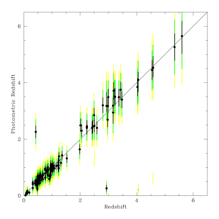
Figure 5: Plot of $z_{\rm ph}$ versus $z_{\rm real}$ including the 1-, 2-, and 3-$sigma$ confidence intervals for each photometric redshift (drawn as increasingly pale shades of grey). Notice the presence of ‘isolated’ low-$z$ pieces of confidence intervals belonging to high redshift objects.

5.1 The catastrophic errors

The term “catastrophic error” has been widely used in the photometric redshift bibliography to identify those cases where the photometric and spectroscopic measurements of the redshift differ in an amount much larger than the expected systematic dispersion (usually at a level greater than three or four times the average photometric redshift dispersion). It has been usually assumed that these cases highlight objects for which the photometric technique fails, possibly due to the lack of sufficiently detailed spectral models to reproduce the intrinsic source spectrum. However, our experience proves (see FS01) that in a large majority of these situations, the spectroscopic value was the one that needed revision.

Nevertheless we know that the redshift probability functions, as described above, can in some cases be multimodal. In such cases, even if our technique is working properly, it may yield results for the best-fit redshift that are distant from the exact value. These events would be considered “catastrophic errors” using the traditional meaning of the term (and also in a purely scientific sense, because they are product of a bifurcation in parameter space). We prefer not to call them “catastrophic”, given that the results–once the error bar is considered–are in fact not in error, and that they can be perfectly individuated using the techniques described in this paper.

Let us study the two particular cases that appeared in Figure 3 as objects with apparently discordant redshifts. It can be seen that in the case of object HDF36478_1256 the photometric and spectroscopic redshifts are in fact compatible to within a $2\sigma$ confidence level. This case was already discussed in FS01, and the conclusion is that it cannot be considered an error (even less a catastrophic error) as the real value is perfectly within the confidence limits of our measurement.

The case of HDF36498_1419 is different. Our redshift probability curve is absolutely incompatible with the redshift claimed in D01. The authors have kindly supplied us with the spectrum, which shows an obvious emission line at $\lambda=5311$ Å. The identification of this line with [Oiii] $\lambda 3727$ is not evident because of the lack of, amongst others, H$\beta$ and [Oiii]$\lambda\lambda$4959,5007 in the covered wavelength range–the authors consider this redshift determination only ‘tentative’. It is true however that other identifications that would put the redshift in agreement with the photometric measurement (Ciii] $\lambda 1909$ or Civ $\lambda\lambda$1548,1551) are also problematic because of the absence of other important lines in the observed range.

We have checked our photometry and do not see any particular problem with the object–it is isolated, and it does not look likely that light from nearby objects could either fool our photometry or produce spurious emission lines. It is not clear what is causing the divergence.

5.2 A check of the confidence intervals

In order to check that the confidence intervals we are calculating are consistent, we perform the following test: for each object, we observe whether the spectroscopic (‘real’) redshift is consistent with our value to within a $1\sigma$, $2\sigma$, $3\sigma$ or none of them. Given the uncertainty about HDF36498_1419 discussed in the previous paragraph, we do not include it in this calculation. The results are listed in Table 2, together with a comparison with the expectations for a pure normal distribution.

Table 2: Analysis of the confidence limits. The columns list the number and fraction of objects whose real redshift is within the 1, 2, and 3 $\sigma$ confidence intervals from our measurement. For comparison, the fractions expected from a normal distribution are also tabulated.

Confidence interval	Obs. number	Obs. fraction	Normal
$<1\sigma$	105/152	$0.691\pm 0.067$	0.6826
$<2\sigma$	145/152	$0.954\pm 0.079$	0.9544
$<3\sigma$	151/152	$0.993\pm 0.081$	0.9974
$>3\sigma$	1/152	$0.007\pm 0.007$	0.0026

It must be noticed that the object which is further than $3\sigma$ is actually only marginally so: the spectroscopic redshift is $z_{\rm sp}=0.483$, with the three sigma interval around $z_{\rm ph}=0.230$ being [0.000–0.473]. In any case, the presence of a $>3\sigma$ deviation in a sample of 151 members is, as indicated in the table, not particularly remarkable.

The results in Table 2 are indicative of the accuracy of our error estimates. We think that this proves that the method here described is a consistent and efficient way to estimate the errors associated to the photometric redshift measurements, and that this method should be used in order to obtain error estimates of any quantity which is measured based on catalogues of photometric redshifts.

6 Conclusions

We have presented a complete analysis of the sources of error present in the photometric redshift determination technique. After showing in a previous paper (FS01) that photometric redshifts are at least as reliable as traditional spectroscopic redshifts when it comes to the measurement of faint galaxies, we show in this paper that the photometric redshifts have an additional advantage: the error in the measurement can be completely characterised by means of a redshift probability function.

We have described how this probability function can be obtained for each individual object, making use of the redshift likelihood function (which accounts for the photometric uncertainties) and of the error component that is added as a systematic effect by our technique. We have modelled this component as a gaussian with variable variance, $\sigma_{z}=\Sigma(1+z)$, and measured the parameter $\Sigma=0.065$ from a large sample of reliable redshifts.

By convolving both error components we obtain a redshift probability function for each object, that easily allows for the determination of confidence intervals associated to the value of the photometric redshift.

We have checked that the confidence limits thus calculated are consistent, and suggest that any quantity to be measured from photometric redshift catalogues in the future should make use of similar techniques, in order to account for the errors inherent to the process of redshift determination.

7 Acknowledgments

We would like to thank our referee, Mark Lacy, for his insightful comments that have improved the clarity of the paper. AFS gratefully acknowledges the support of the European Commission through a Marie Curie Fellowship.

References

- [Baum 1962] Baum, W.A. 1962, in Problems of Extragalactic Research IAU Symp. 15 (New York: Macmillan), p. 390
- [Benítez 2000] Benítez N. 2000, ApJ, 536, 571
- [Butchins 1981] Butchins S. A. 1981, A&A, 97, 407
- [Cohen et al. 2000] Cohen J.G., Hogg D.W., Blandford R., Cowie L.L., Hu E.M., Songaila A., Shopbell P., Richberg K. 2000, ApJ, 538, 29 (C00)
- [Cohen 2001] Cohen J.G. 2001, AJ, 121, 2895 (C01)
- [Dawson et al. 2001] Dawson S., Stern D., Bunker A.J., Spinrad H., Dey A. 2001, AJ, 122, 598 (D01)
- [Fernández-Soto et al. 2001] Fernández-Soto A., Lanzetta K.M., Chen H.-W., Pascarelle S.M., Yahata, N. 2001, ApJSS, 135, 41 (FS01)
- [Fernández-Soto, Lanzetta, Yahil 1999] Fernández-Soto A., Lanzetta K.M., Yahil A. 1999, ApJ, 513, 34 (FLY99)
- [Fontana et al. 2000] Fontana A., D’Odorico S., Poli, F., Giallongo E., Arnouts S., Cristiani S., Moorwood A., Saracco P. 2000, AJ, 120, 2206
- [Furusawa et al. 2000] Furusawa H., Shimasaku K., Doi M., Okamura S. 2000, ApJ, 534, 624
- [Gwyn & Hartwick 1996] Gwyn S.D.J., Hartwick F.D.A. 1996, ApJ, 468, L77
- [Koo 1981] Koo. D.C. 1981, PhD Thesis, University of California
- [Lanzetta, Yahil, Fernández-Soto 1996] Lanzetta K.M., Yahil A., Fernández-Soto A. 1996, Nature, 381, 759
- [Lanzetta, Fernández-Soto, Yahil 1998] Lanzetta K.M., Fernández-Soto A., Yahil A. 1998, in Proc. STScI 1997 May Symp., The Hubble Deep Field, ed. Livio M., Fall S.M., Madau P. (Cambridge: Cambridge University Press) (LFY98)
- [Loh & Spillar 1986] Loh E.D., Spillar E.J. 1986, ApJ, 303, 154
- [Massarotti et al. 2001] Massarotti M., Iovino A., Buzzoni A., Valls-Gabaud D. 2001, A&A, in press
- [Sawicki, Lin, Yee 1997] Sawicki M.J., Lin H., Yee H.K.C. 1997, AJ, 113, 1
- [Wang, Bahcall & Turner 1998] Wang Y., Bahcall N., Turner E.L. 1998, AJ, 116, 2081
- [Williams et al. 1996] Williams, R.E., et al. 1996, AJ, 112, 1335
- [Yahata et al. 2000] Yahata N., Lanzetta K.M., Chen H.-W., Fernández-Soto A., Pascarelle S., Yahil A., Puetter R.C. 2000, ApJ, 538, 493 (Y00)