Far-infrared and molecular line observations of Lynds 183 - studies of cold gas and dust

We have mapped the dark cloud L183 in the far-infrared at 100$\mu$m and 200$\mu$m with the ISOPHOT photometer aboard the ISO satellite. The observations make it possible for the first time to study the distribution and properties of the large dust grains in L183 without confusion from smaller grains. The observations show clear colour temperature variations which are likely to be caused by changes in the emission properties of the dust particles. In the cloud core the far-infrared colour temperature drops below 12 K. The data allow a new determination of the cloud mass and the mass distribution based on dust emission. The estimated mass within a radius of 10$\arcmin$ from the cloud centre is 25 $M_{\sun}$. We have mapped the cloud in several molecular lines including DCO+(2–1) and H¹³CO+(1–0). These species are believed to be tracers of cold and dense molecular material and we detect a strong anticorrelation between the DCO+ emission and the dust colour temperatures. In particular, the DCO+(2–1) emission is not detected towards the maximum of the 100$\mu$m emission where the colour temperature rises above 15 K. The H¹³CO+ emission follows closely the DCO+ distribution but CO isotopes show strong emission even towards the 100$\mu$m peak. Detailed comparison of the DCO+ and C¹⁸O maps shows sharp variations in the relative intensities of the species. Morphologically the 200$\mu$m dust emission traces the distribution of dense molecular material as seen e.g. in C¹⁸O lines. A comparison with dust column density shows, however, that C¹⁸O is depleted by a factor of $\sim$1.5 in the cloud core. We present results of $R$- and $B$-band starcounts. The extinction is much better correlated with the 200 $\mu$m than with the 100 $\mu$m emission. Based on the 200 $\mu$m correlation at low extinction values we deduce a value of $\sim$17^m for the visual extinction towards the cloud centre where no background stars are observed anymore.

1 Introduction

The distribution of material in dense interstellar clouds can be traced by either molecular line emission or the continuum emission from dust particles. The analysis of line spectra is complicated by radiative transfer effects. The emission of radiation depends on local properties like density and kinetic temperature. Based on these parameters, the observed line intensities can be predicted with radiative transfer modelling. In practice, the density structure of the sources is, however, unknown and e.g. small scale density and velocity variations can seriously affect the observed intensities. Secondly, the ratio between the abundance of the tracer and the total gas mass is only known approximately and it can change even within one source. The chemical reactions depend on density and temperature (Millar et al. millar97 (1997); Lee et al. lee96a (1996)) and therefore the chemistry of a dark cloud cores will differ from the chemistry in the surrounding warmer material.

Molecular abundances depend on the strength of the ultraviolet radiation field via processes such as photodissociation. The radiation is weakened by dust extinction and by the self-shielding of the molecules and this introduces radial abundance gradients. Selective photo-dissociation can lead to strong abundance variations between different CO isotopes and can even affect the excitation of the molecules (Warin et al.warin96 (1996)) The abundances change even as a function of time (Leung et al. 1984; Herbst & Leung 1989, 1990; Bettens et al. 1995) and the observed abundances have been used as a ‘chemical clock’ to determine the evolutionary stage of sources (e.g. Stahler stahler84 (1984); Lee et al. lee96b (1996)). Observations of e.g. TMC-1 show clear anti-correlation between carbon bearing and oxygen bearing molecules (Pratap et al. pratap97 (1997)). This can be compared with models (e.g. Bergin et al. bergin95 (1995), bergin96 (1996)) which show that CS and long carbon chain molecules are produced preferentially at early times, while SO abundance rises only much later.

The role of dust grains in chemical evolution is important but not yet well understood. In dark cores some molecules can freeze onto the dust grains and this causes the under-abundance of the molecules in the gas phase. CO abundances can decrease by more than a factor of ten (Gibb & Little gibb98 (1998)). In the cold cores, the abundance of deuterated species, e.g. DCO+ are enhanced. This fact has been used to identify condensations in the earliest stages of star formation, before the birth of protostars again increases the temperatures (e.g. Loren et al. loren90 (1990)). The abundance ratio [DCO+]/[HCO+] depends also on the abundance of free electrons and can therefore also be used to determine this quantity (e.g. Guélin et al. guelin77 (1977), guelin82 (1982); Watson watson78 (1978); Wootten wootten82 (1982); Anderson et al. anderson99 (1999)). The electron abundance is an important parameter since, through ambipolar diffusion, it affects the timescales of physical cloud evolution and eventually the rate of the star formation (Caselli et al. caselli98 (1998)).

The analysis of far-infrared dust continuum observations is in principle more straightforward. The emission is optically thin and the intensity directly related to the dust column density. At wavelengths 100-200$\mu$m the radiation is emitted mainly by the classical large grains, with a possible small contribution at 100 $\mu$m by the ‘very small grains’. The large grains heated by the normal interstellar radiation field settle to a temperature of $\sim$17 K and the maximum of the spectral energy distribution is close to 200$\mu$m. The temperature of the small grains fluctuates and most of the radiation is at shorter wavelengths ($\lambda<100\mu$m). In the model of Désert et al. (desert90 (1990)) some 10% of the infrared emission at 100$\mu$m comes from very small dust grains.

The large grains are well mixed with the gas phase (Bohlin et al. bohlin78 (1978)) and the FIR emission can be used to trace the gas distribution. The dust emission corresponding to a given column density varies depending on the composition and temperature of the dust. The far-infrared colour temperature has been observed to drop towards the centre of many dark cores (e.g. Clark et al. clark91 (1991); Laureijs et al.laureijs91 (1991)) and even cirrus type clouds (Bernard et al. bernard99 (1999)). It is clear that the variations cannot be entirely due to a reduced radiation field, i.e. the observed colour temperature variations indicate a change in the grain properties. In the cloud cores, the dust particles may grow through coagulation, and in this case the associated change in the grain emissivity could explain part of the colour temperature variations (e.g. Meny et al. meny00 (2000); Cambrésy et al. cambresy01 (2001)). Changes in the dust properties cause uncertainties to the column density estimates. These are, however, smaller than those associated with the analysis of optically thick molecular lines.

Most of the listed problems can be addressed by comparing observations of molecular line emission with far-infrared dust emission. In this paper we present such a study of the dark cloud L183.

1.1 L183

L183 (L134N) is a well known dark cloud belonging to a high latitude cloud complex (Galactic coordinates ($l$, $b$)=(6.0, 36.7)). The distance of the cloud has been estimated to be 100 pc (Mattila mattila79 (1979), Franco franco89 (1989)) although a distance of 160 pc has also been used (Snell snell81a (1981)). We adopt $d$=100 pc. Extinction towards the centre of L183 is at least $A_{\rm V}\sim$6 (Laureijs et al. laureijs91 (1991)) and may exceed $A_{\rm V}=$10. The cloud core is surrounded by an extended low extinction ($A_{\rm V}<$1) envelope.

L183 was observed in CO(1–0) and ¹³CO(1–0) by Snell (snell81 (1981)), in NH₃ by Ungerechts et al. (ungerechts80 (1980)) and in several lines including C¹⁸O(1–0) and H¹³CO+(1–0) by Swade (1989a ; 1989b ). The ¹³CO line map shows a cometary shape with the head of the globule pointing north in equatorial coordinates ($\sim$galactic east). This is also the densest part of the cloud. The cloud has a sharp edge towards the north, but in the southern part the strong ¹³CO and especially the ¹²CO emission continues in the tail that points towards L1780. Together, the region containing clouds L134, L169, L183, L1780 is sometimes called the L134 complex. NH₃ and C₃H₂ emission is concentrated into the head region and ammonia emission is restricted to a very narrow ridge running from south to north. The usual centre position given for the cloud, (RA=15^h51^m30^s Dec=-2$\degr$43$\arcmin$31$\arcsec$, 1950.0) is close to the centre of the ammonia emission where density reaches a few times 10⁴ cm^-3 (Swade 1989b ). In recent years the cloud has been observed in a number of molecular lines (see e.g. Swade & Schloerb swade92 (1992); Turner et al. turner99 (1999), turner00 (2000) and Dickens et al. dickens00 (2000) and references therein).

The infrared emission from L183 was studied by Laureijs et al. (laureijs91 (1991); laureijs95 (1995)) based on the IRAS data. The 60$\mu$m emission is detected only in a narrow layer surrounding the cloud core. Based on the upper limit of the I(60$\mu$m)/I(100$\mu$m) ratio, an upper limit of 15 K was derived for the colour temperature assuming a $\nu^{2}$ emissivity law. However, at 60$\mu$m, most of the emission comes from small dust particles, and the colour temperature is not directly related to the physical grain temperature. In the cloud core the lack of 60$\mu$m emission was interpreted as evidence for mantle growth. Ward-Thompson et al. (wt94 (1994); wt00 (2000)) have made sub-millimetre continuum observations of the cloud and have detected two point sources close to the cloud centre. Lehtinen et al. (lehtinen00 (2000)) have studied the properties of the sources using far-infrared observations made with ISO.

In this paper we study the dark cloud L183 using 100 $\mu$m and 200 $\mu$m maps and new molecular line observations. The far-infrared observations were carried out with the ISOPHOT instrument aboard the ISO satellite. Both 100$\mu$m and 200$\mu$m are dominated by emission from classical large grains and this makes it possible, for the first time, to study the variations in the properties of the large grains without confusion from smaller size dust populations. The far-infrared observations enable us to determine the mass distribution of L183 independently from the molecular line data which may be affected by chemical fractionation and other systematic effects. The dust distribution will be compared with molecular line observations which include new ¹²CO, ¹³CO and C¹⁸O observations that cover the entire cloud L183. The correlations with dust column densities will be used to determine the degree of C¹⁸O depletion in the core of L183. New DCO+(2–1) and H¹³CO+(1–0) mappings have been made with higher spatial resolution than what were previously available. DCO+ is known to be a tracer of cold gas and we will determine the correlations between DCO+ and dust emission, especially the FIR colour temperatures. We will also study the variations in the intensity ratio of DCO+ and H¹³CO+. Finally, we present results of $R$- and $B$-band star counts and a comparison between the extinction and the far-infrared emission.

2 Observations and data processing

2.1 FIR observations

Far-infrared observation of L183 were done with the ISOPHOT photometer (Lemke et al. lemke (1996)) aboard the ISO satellite (Kessler et al. kessler (1996)). Two 30$\arcmin\times 30\arcmin$ maps were made in the PHT22 staring raster map mode with filters C_100 and C_200. The reference wavelengths of the filters are 100 $\mu$m and 200 $\mu$m and the respective pixel sizes $\sim$44$\arcsec$ and 89$\arcsec$.

Additional narrow strips running from NW towards the cloud centre were observed at 80$\mu$m, 100$\mu$m, 120$\mu$m, 150$\mu$m and 200$\mu$m. The analysis of these observations will be presented by Lehtinen et al. (in preparation).

Comparison of the ISOPHOT 100 $\mu$m observations with the 100 $\mu$m IRAS ISSA maps showed peculiar scatter with two separate branches in the ISOPHOT vs. IRAS relation. The calibration of the ISOPHOT observations was done with Fine Calibration Source (FCS) measurements that were done before and after the actual mapping and a linear interpolation was performed to determine the detector responsivity at each map position. The detector signals did not, however, stabilize during FCS measurements and this leads to some uncertainty. A 5% change in the relative responsivities of the two FCS measurements was found to be enough to minimize the scatter relative to the IRAS map. The average responsivity over the map was not changed. The resulting relation between ISOPHOT and IRAS ISSA surface brightness values is shown in Fig. 1. Because of the large temperature variations the relation between 100$\mu$m and 200$\mu$m surfaces brightness values shows a significantly larger scatter (see Fig. 2). This is also decreased by the 5% adjustment of the 100$\mu$m responsivities.

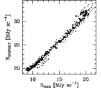
Figure 1: The relation between the 100$\mu$m ISOPHOT and IRAS ISSA surface brightness values. The ISOPHOT time-ordered data have been tilted 5% in order to obtain lowest dispersion when compared with IRAS values (see text). The slope of the fitted line is 1.09. No zodiacal light has been subtracted from the ISOPHOT values.

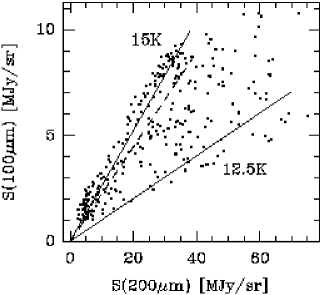
Figure 2: Observed 100 $\mu$m surface brightness as the function of the 200 $\mu$m values. The diffuse background determined from regions with lowest surface brightness has been subtracted from the observed values and the 100 $\mu$m data are convolved to the resolution of the 200 $\mu$m observations.. The solid lines correspond to dust colour temperatures 12.5 K and 15.0 K. The dashed line shows the least squares line fitted to points $S$(200 $\mu$m)$<$30 MJy sr^-1

The 100 $\mu$m map was finally rescaled to the DIRBE surface brightness scale by multiplying the values with 0.85. The scaling was established by correlating DIRBE, IRAS and ISOPHOT surface brightness values in the area. Details of the procedure are given in Lehtinen et al. (in preparation). The 200 $\mu$m observations were calibrated using the FCS measurements which were of good quality. The uncertainty in the absolute calibration of the 200 $\mu$m map is expected to be below 20% (see García-Lario garcia00 (2000)). The final far-infrared maps are shown in Fig. 3.

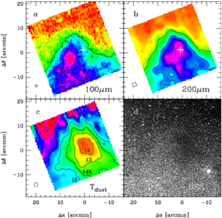
Figure 3: a-b) The 100$\mu$m and 200$\mu$m ISOPHOT maps of the cloud L183. The cross indicates the position of the continuum source detected by Ward-Thompson et al. (wt94 (1994). The (0,0) position is RA=15^h51^m30^s DEC=-2$\degr$43$\arcmin$31$\arcsec$. In the case of 100 $\mu$m the contours are at 15 and 20 MJy sr^-1 and for 200 $\mu$m the contour levels are 30, 50 and 70 MJy sr^-1. The small squares at the lower left corner indicate the pixel sizes, 44$\arcsec$ for 100 $\mu$m and 89$\arcsec$ for the 200 $\mu$m map. c) The map of dust colour temperature calculated from the 100$\mu$m and 200$\mu$m ISOPHOT observations. The contours are at intervals of 1 K starting with 12 K. The effective resolution is 100$\arcsec$. d) blue image from the Digitized Sky Survey.

2.2 Molecular line observations

The molecular line observations were made with the SEST telescope during two session in February 1998 and February 1999. During the first observing period, the cloud was mapped in the lines ¹²CO(2–1), ¹³CO(1–0) ¹³CO(2–1), C³⁴S(2–1) and C¹⁸O(1–0). Due to a problem with the receiver, the C¹⁸O(2–1) map remained uncompleted. In February 1999 observations were made in the DCO+(2–1) and H¹³CO+(1–0) lines.

During observations, the pointing was checked every two or three hours by observing bright SiO maser sources. The estimated pointing uncertainty is less than 5$\arcsec$. Most observations were made in the frequency switching mode with a frequency throw 6 MHz. The chopper-wheel method was used for calibration and observed intensities are given in T${}^{*}_{\rm A}$ units. The typical rms noise levels are given in Table 1.

The ¹²CO, ¹³CO and C¹⁸O maps cover practically the entire cloud L183 as seen in optical extinction. In the southern part, a fairly strong molecular line emission continues up to the edge of the map. The H¹³CO+(1–0) and DCO+(2–1) maps are smaller in size, but particularly in the case of DCO+, they cover the whole region of significant emission. At the map boundaries, the DCO+ intensity has dropped from a peak value $T_{\rm A}\approx$1.1 K to $\sim$0.25 K or below.

Table 1: Summary of observed molecular emission lines. The columns are: (1) transition, (2) beam size, (3) spectral resolution (4) number of observed positions and (5) the average rms noise.

line	FWHM	$\Delta v$	positions	$<\sigma_{\rm RMS}>$
	($\arcsec$)	(km s-1)		(K)
12CO(2–1)	23	0.054	83	0.17
13CO(1–0)	46	0.114	83	0.069
13CO(2–1)	24	0.057	532	0.14
C18O(1–0)	46	0.114	533	0.10
H13CO+(1–0)	57	0.144	174	0.040
DCO+(2–1)	35	0.087	176	0.061

2.3 Star counts

The optical extinction in the L134 cloud complex was determined by means of star counts using a blue (IIaO + GG385 filter) and a red (IIIaF + RG630) ESO Schmidt plate (Plate Nos.3713 and 3714) which were obtained on 16 April 1980. Star counts were performed using a reseau size of 2.8$\arcmin\times$2.8$\arcmin$. The total number of stars down to the limiting magnitude of each plate was counted (see Bok bok56 (1956) for the method).

In order to derive the extinction, the function $N(m)$ is needed, i.e. the number of stars per sq.degree with magnitude $\leq m$ in a transparent comparison area close to the dark nebula. The tables of van Rhijn (rhijn29 (1929)) have often been used for this purpose (see Bok bok56 (1956)). In the present case it was better to use the RGU photometric catalogue of Becker and Fenkart (becker76 (1976)) for Selected Area 107 which is located close ($l$=5.7 deg, $b$= 41.3 deg) to the L134 complex. The R and G band star numbers for SA 107 were extracted from the compilation by Bahcall et al. (bahcall85 (1985)). These $N(m)$ curves were extrapolated beyond the limiting magnitudes $R$=17.5 and $G$=18.5, and were corrected to account for the somewhat different Galactic latitude ($b$ = 36 deg) of the L134 complex by using the tabulated results of Bahcall and Soneira (bahcall80 (1980)) for their Galaxy model in the $B$ and $V$ bands.

An essential parameter of the $logN(m)$ vs. $m$ calibration curve is its slope at the limiting magnitude of the star counts. In our case this slope turned out to be 0.22 at $G_{\rm lim}$ = 20.1 mag and $R_{\rm lim}$=19.3 mag, respectively. We note that the $G$ and $R$ passbands of the Basle RGU photometric system with effective wavelengths of 463 and 638 nm are close enough to the wavelength ranges of our blue (380–480 nm) and red plate (630–690 nm).

The resulting extinction maps are shown in Fig. 4.

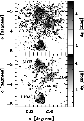
Figure 4: The extinction maps of the L134 dark cloud complex derived from starcounts in the $R$- (lower frame) and $B$-bands (upper frame). The area mapped with ISOPHOT is indicated with a square. Individual clouds L134, L183 and L169 are indicated in the figure. The contour levels are at 1, 2 and 4^m.

3 Observational results

3.1 FIR maps

The main structure seen in the far-infrared maps (Fig. 3a-b) is a wedge pointing northwards. The intensity is highest close to the head of the wedge, and drops rapidly towards the north and more slowly towards the south. There are clear differences in the distributions at 100$\mu$m and 200$\mu$m. There are two broad 200$\mu$m maxima, one close to the optical extinction peak and previously known mm- and sub-mm continuum source (Ward-Thompson et al. wt94 (1994)) and another $\sim$5$\arcmin$ towards SE. In the 100$\mu$m map only the latter peak is visible. The relative strength of the 200$\mu$m emission is larger in the north, west and southwest while the 100$\mu$m emission is stronger in the southeast. In the west the 100$\mu$m emission seems to extend further out, although the surface brightness is already close to the background level.

The 200$\mu$m emission is caused entirely by the large classical grains and at 100$\mu$m the contribution from small grains is expected to be small, $\la$10%. Dust temperature map was derived assuming that large grains emit according to a modified black body radiation $\nu^{2}B(\nu,T_{\rm d})$. The background corresponding to the lowest surface brightness values within the mapped area was first subtracted. Average 100$\mu$m surface brightness values were calculated corresponding to each 200$\mu$m measurement. Values were colour corrected and the dust temperature was obtained by the fitting of the modified Planck curve. Since the colour correction depends weakly on the assumed temperature the procedure was repeated once using the temperature derived from the initial fit.

The dust temperature in Fig. 3c has a well defined minimum close to the position of the continuum source. The minimum temperature in the 200$\mu$m core is below $\sim 12$ K while in the north and west the temperature rises rapidly to $\sim$16 K. There is no temperature maximum at the 100 $\mu$m emission maximum and the position does not differ in any way from its surroundings. The 5% tilting of the 100$\mu$m map (Sect. 2.1) changed the temperatures by up to $\sim$1 K at the eastern and western borders (the first and last scan lines in the map). As the average responsivity was not changed the temperature in the centre, i.e. in the cold core, was not affected.

The correlation between 100 $\mu$m and 200 $\mu$m surface brightness values (Fig. 2) shows considerable scatter. The scatter was somewhat reduced by the correction applied to the relative responsivity of the 100 $\mu$m FCS measurements (see Sect. 2.1). A further modification of the responsivities would have very little effect on the scatter, which is caused by true variations of the dust properties. The variations are reflected in the dust temperature distribution.

A linear least squares fit to the data points in Fig. 2 gives a relation $S_{\rm fit}$(200 $\mu$m)= (0.14$\pm$0.01) S(100 $\mu$m) + (1.30$\pm$0.06). The fitting procedure takes into account the uncertainty in both variables. The statistical error of the intercept in particular is small compared with the uncertainty due to calibration and the background subtraction. Data at positions where the background subtracted values of $S$(200 $\mu$m) were below 30 MJy sr^-1 (i.e. outside the cloud core) give a relation $S_{\rm fit}$(200 $\mu$m)= (0.22$\pm$0.01) S(100 $\mu$m). The limit of 30 MJy sr^-1 at 200 $\mu$m corresponds approximately to the 50 MJy sr^-1 contour in Fig. 3 where no background subtraction was made. According to Fig. 4 the excluded area corresponds also to the region with highest extinction, $A_{\rm B}\ga$4^m. Based on the derived dependence we calculate $\Delta S(200\mu$m)=$S_{\rm obs}$(200 $\mu$m)-$S_{\rm fit}$(200 $\mu$m), which is the difference of the observed 200 $\mu$m surface brightness and the predicted value based on the 100 $\mu$m data. The resulting map of $\Delta S$(200 $\mu$m) (Fig. 5) shows the 200 $\mu$m excess that can be due to either cold dust or dust with enhanced emissivity at the longer wavelength.

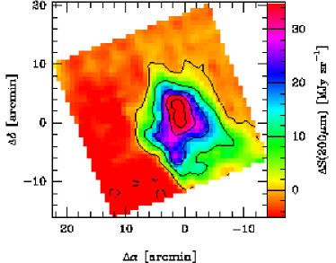
Figure 5: Distribution of $\Delta S(200\,\mu$m). $\Delta S(200\,\mu$m) is the difference between the observed 200 $\mu$m surface brightness and the least squares prediction calculated from the 100 $\mu$m values.

The 200 $\mu$m optical depth was calculated from the observed intensities as $\tau(200\,\mu$m)=$S/B(T)$. Here $B(T)$ is the black body intensity at temperature $T$ as read from Fig. 3c. The resulting map, which shows the column density distribution of large dust grains, is rather similar to the 200 $\mu$m intensity distribution. Due to its low colour temperature, however, the main core is much more pronounced. The region of the 100 $\mu$m peak is correspondingly weaker and is visible only as an extension of the main core. Fig. 6 shows the 200 $\mu$m surface brightness in relation to the 200 $\mu$m optical depth. While the SE core is also visible as a separate intensity peak in the 200 $\mu$m map, the large grains are clearly concentrated in the NW core. A similar relation is seen between the 200 $\mu$m emission and the dust colour temperature. In the temperature map the SE peak is completely invisible.

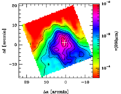
Figure 6: 200 $\mu$m surface brightness (contours) and the calculated optical depths at the same wavelength. The contours start at 15 MJy sr^-1 and are drawn at intervals of 15 MJy sr^-1.

The cloud mass was calculated from the 200 $\mu$m optical depth using the value $\sigma_{\rm H}=2.5\cdot 10^{-25}$cm² for the effective dust cross section per hydrogen atom at 200 $\mu$m (Lehtinen et al. lehtinen98 (1998)). The mass within 10$\arcmin$ of position (0,0) is 25 $M_{\sun}$ for $d=$100 pc. Alternatively, the mass contained within the contour $\tau$(200 $\mu$m)=6$\cdot$10^-4 is 28 $M_{\sun}$. The main uncertainty is in the value of $\sigma_{\rm H}$ and use of the formula given by Boulanger et al. boulanger96 (1996), $\sigma_{\rm H}=10^{-25}(\lambda/250\mu m)^{-2}$cm^-2, would result in some 50% higher mass estimates. We note that the latter $\sigma_{\rm H}$ value is for diffuse medium, while the Lehtinen et al. value is for a dense globule similar to L183.

As shown in Fig. 5, there is a clear 200$\mu$m excess in the centre of L183. This could be due to a decrease in the physical temperature of the dust grains induced by the decreasing intensity of the radiation field, or by increased overall FIR emissivity of the grains. Another possibility would be a change in grain properties, i.e. increased emissivity at the longer wavelength, leading to a change of the dust emissivity index. Both explanations are related to the increasing density in the cloud centre. Both theoretical studies (e.g. Ossenkopf ossenkopf93 (1993); Wright wright87 (1987)) and recent PRONAOS observations (Bernard et al. bernard99 (1999); Stepnik et al. stepnik01 (2001)) indicate that dust emission properties are likely to change in dense and cold clouds. This could be the result of grain growth, or possibly the formation of grain aggregates. In a forthcoming paper (Juvela et al., in preparation) we will study the far-infrared dust emission using radiative transfer models. Further discussion about the dust temperatures and changes in the dust emissivity law will be deferred to that paper.

3.2 Distribution of molecular line emission

Figure 7 shows the distributions of the integrated antenna temperature in lines ¹²CO(2–1), ¹³CO(2–1), C¹⁸O(1–0), H¹³CO+(1–0) and DCO+(2–1).

The CO lines follow the general morphology seen in the maps by Snell (snell81 (1981)) and Swade et al. (1989a ). The ¹²CO emission increases towards the south while C¹⁸O and ¹³CO(1–0) delineate the dense core close to the given centre position. The ¹³CO(1–0) emission extends towards the southwest, however, where the ¹³CO(2–1) emission peaks well outside the core seen in C¹⁸O. The distributions of H¹³CO+(1–0) and DCO+(2–1) are clearly different from the CO species. The distribution of H¹³CO+(1–0) is similar to what was seen by Guélin et al. (guelin82 (1982)). However, due to the better resolution of the present study the emission area is better resolved and the map is more structured. There is a second emission peak south of the centre at position (1,-4). The morphology of the DCO+(2–1) emission follows closely that of the H¹³CO+(1–0). The emission is concentrated along a narrow, but clearly resolved ridge with some extension west of the centre position. The western extension is seen in both lines, although it was not visible in the Guélin et al. H¹³CO map. In the centre, the DCO+ emission seems to be more concentrated around the peak position. However, this is mainly due to the smaller beam size of the DCO+ observations.

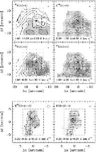
Figure 7: Maps of the integrated line areas: ¹²CO(1–0), C¹⁸(1–0), ¹³CO(1–0), ¹³CO(2–1), H¹³CO+(1–0) and DCO+(2–1). The dashed lines in each frame indicate the location of the DCO+ core

Maps of C¹⁸O(1-0), ¹³CO(1-0) and ¹³CO(2-1) emission in different velocity intervals are shown Figs. 8–10. In the lowest radial velocity bin, C¹⁸O emission is seen both northeast of the position (0,0) and towards the western edge of the map. In the interval  2.0-2.5 km s^-1, strong emission still exists in the western part of the map. The main core is visible in all three higher velocity intervals. Below 3 km s^-1 the emission extends between the positions of the 100 $\mu$m and 200 $\mu$m maxima (see Fig. 3) while at the highest radial velocities the emission is concentrated around position (0,0) only. The same general morphology and dependence on the radial velocity is repeated in the ¹³CO maps. The relative intensity of the ¹³CO lines is, however, higher in the south. As the radial velocity increases the emission maximum moves over the C¹⁸O core from northeast to southwest.

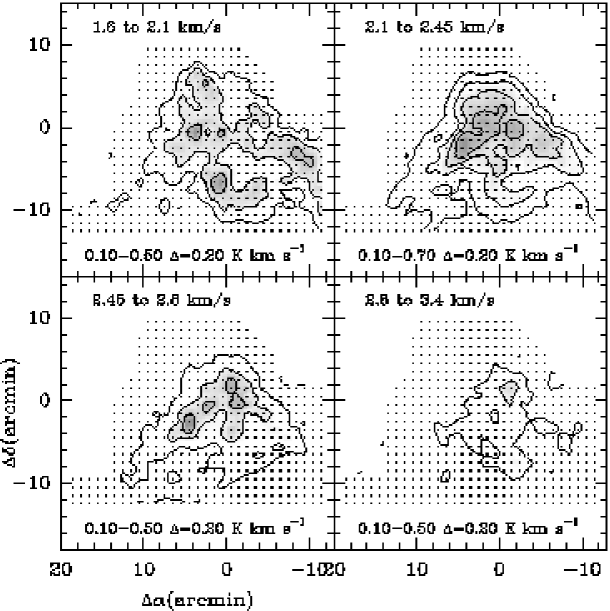
Figure 8: C¹⁸O(1–0) integrated antenna temperature in four velocity intervals. The velocity intervals are given in the upper part of the panels. The range of contour levels and the step between consecutive contours are written at the bottom of the panels.

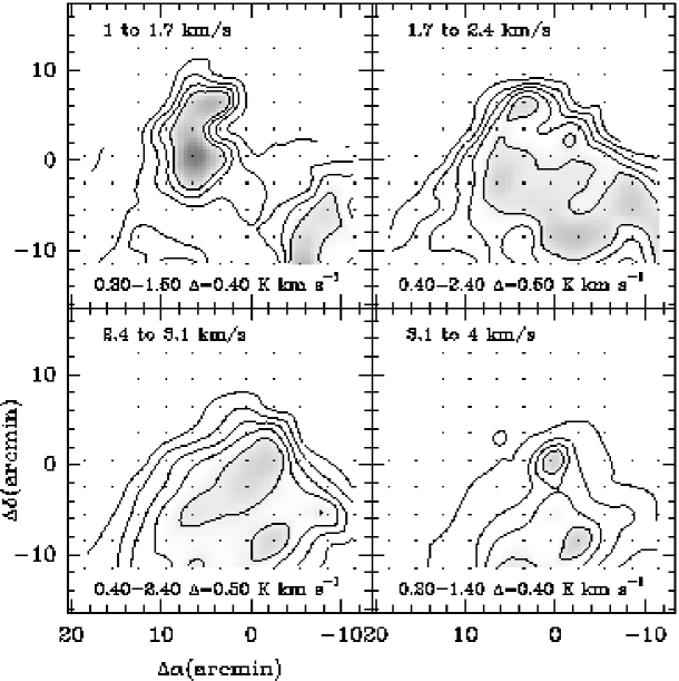
Figure 9: ¹³CO(1–0) integrated antenna temperature in four velocity intervals. The velocity intervals and the contour values are indicated in the panels.

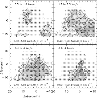
Figure 10: ¹³CO(2–1) integrated antenna temperature in four velocity intervals. The velocity intervals and the contour values are indicated in the panels.

The DCO+(2–1) and H¹³CO+(2–1) in Figs. 11-12 show similar behaviour. At low velocity, the emission is concentrated in the south around position (2,-3) while at other velocities the maximum is reached close to position (0,0). There are also some differences, and H¹³CO+ is relatively stronger around the emission peak in the south.

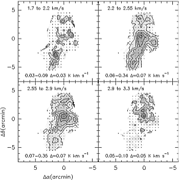
Figure 11: DCO+(2–1) integrated antenna temperature. The velocity intervals and the contour values are indicated in the panels.

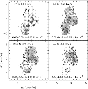
Figure 12: H¹³CO+(1–0) integrated antenna temperature. The velocity intervals and the contour values are indicated in the panels.

4 Models of radiative transfer and column densities of molecular gas

LTE column density estimates were computed based on the ¹³CO(1–0) and C¹⁸O(1–0) observations. The derived excitation temperatures are between 7 and 9 K. Compared with the rest of the cloud, the excitation temperature seems to be systematically  1 K lower in the northern part close to the column density maximum. However, the difference is small and we derive column densities assuming a constant excitation temperature of $T_{\rm ex}$=8.4 K. The LTE column densities were calculated according to the formula given by Harjunpää et al. (harjunpaa96 (1996)) and are shown in Fig 13. In the conversion from C¹⁸O to H₂ column densities, a fractional C¹⁸O abundance of 1$\cdot$10^-7 was assumed, corresponding to the quiescent cloud positions in Harjunpää et al. (harjunpaa96 (1996)) and Frerking et al. (frerking82 (1982)).

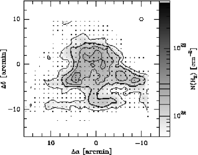
Figure 13: LTE hydrogen column density as derived from the ¹³CO(1–0) and C¹⁸O(1–0) observations. The contours start at value N(H₂)=5$\cdot$10²¹cm^-2 and are drawn at intervals of 5$\cdot$10²¹cm^-2 (the thick contour line denotes the value N(H₂)=1$\cdot$10²²cm^-2).

From the derived column densities we obtain a value of $\sim$47 M_☉ for the cloud mass within 10$\arcmin$ of the centre position, or some 35 M_☉ for the mass contained within the contour $N({\rm H}_{2}$)=1.0$\cdot$10²² cm^-2.

For comparison, the C¹⁸O and ¹³CO emission were modelled with spherically-symmetric model clouds where the radiative transfer problem was solved with Monte Carlo methods (see Juvela et al. juvela97 (1997)). While spherical symmetry presents an extreme simplification of true density distribution, the models will still be more realistic than the assumptions underlying the LTE calculations (see e.g. Padoan et al. padoan00 (2000)). The model clouds are assumed to be isothermal with radial density dependence of $n\sim r^{-1.5}$ and with density contrast 20 between cloud centre and outer boundary. The free parameters of the models were the cloud size, central density and the kinetic temperature. The C¹⁸O(1–0), ¹³CO(1–0) and ¹³CO(2–1) spectra within 10$\arcmin$ radius of the position (0,0) were compared with spectra calculated from the radiative transfer model and the free parameters were adjusted in order to obtain the best fit. The gas distribution is asymmetric with respect to the centre position and the ¹³CO emission is displaced with respect to C¹⁸O. Therefore, the results can not be expected to be very accurate. However, although the listed free parameters are not well constrained, the column density estimates should be more reliable.

Assuming a constant kinetic temperature of 10 K, the best fit was obtained with a model having a mass of 40 $M_{\sun}$. The mass estimate is not very sensitive to the assumed kinetic temperature. A similar model with $T_{\rm kin}$ increasing linearly from 8.0 K in the centre to 15 K on the cloud surface resulted in a mass estimate of 34 $M_{\sun}$. The quality of the fit was, however, marginally better in the isothermal model.

The spectral lines do not show signs of cloud collapse. Several ¹³CO spectra have double peaked, asymmetric profiles but comparison with optically thinner C¹⁸O indicates that these are caused by separate emission components rather than self-absorption. Gaussian fits give average linewidths of $\sim$0.7 km s^-1 for both ¹³CO(2–1) and C¹⁸O(1–0). The virial mass was estimated according to equation

$$M_{\rm vir}=(\frac{\sigma_{\rm 3D}}{C})^{2}R,$$ (1)

where $\sigma_{\rm 3D}$ is the three-dimensional velocity dispersion, $R$ the radius of the cloud and $C$ is a constant depending on the assumed model of the cloud. The value of $C$ is 0.0508 km s^-1 $\sqrt{pc/M_{\sun}}$ for a homogeneous sphere and 0.0463 km s^-1 $\sqrt{pc/M_{\sun}}$ for density distribution $n\sim r^{-1}$ (see Liljeström liljestrom91 (1991)). Assuming gas temperature 13 K and $R\sim 10\arcmin$ the observed velocity dispersion corresponds to virial masses of 54 $M_{\sun}$ and 44 $M_{\sun}$ for the two models. In the presence of noise the FWHM derived from gaussian fits may, however, be biased and the average FWHM read directly from the spectra is smaller, $\sim$0.5 km s^-1, lowering the virial mass estimates to 36 $M_{\sun}$ and 30 $M_{\sun}$, correspondingly. The previous analysis ignores both the external pressure and the presence of velocity gradients. The cloud is, however, approximately in virial equilibrium. Even though the cloud as a whole may not be collapsing it can still contain collapsing fragments. In fact, there is evidence of several pre-protostellar cores in L183 (Lehtinen et al. lehtinen00 (2000)).

We will return to the modelling of the molecular line data in a future paper (Juvela et al., in preparation) where radiative transfer models will also be constructed for the far-infrared dust emission.

4.1 Comparison of FIR and molecular line maps and column densities

Fig. 14 shows the distribution of FIR surface brightness relative to the intensity of the C¹⁸O(1–0) lines. The 200$\mu$m intensity closely follows the C¹⁸O emission. The peak positions do coincide and the second 200$\mu$m maximum in the southeast as well as fainter extensions towards south and towards southwest have corresponding features in the line map. The 200$\mu$m emission extends, however, somewhat further in the north while the C¹⁸O is relatively stronger in the southwest. With respect to the 200 $\mu$m peak the C¹⁸O(1–0) maximum is displaced slightly towards the southwest. Further towards the southwest, the C¹⁸O is again well traced by the FIR emission. The second C¹⁸O(1–0) peak at position (4,-2) coincides with the second 200 $\mu$m peak. There is, however, a third 200 $\mu$m peak at (1,-6) which does not have a direct counterpart in the molecular line emission. The peak corresponds to just one pixel above the diffuse background and could even be caused by a single extragalactic source. The 100$\mu$m peak traces the eastern extension of the C¹⁸O distribution. Apart from this there is a clear lack of correlation with molecular line emission, especially within the C¹⁸O core.

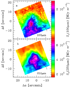
Figure 14: The far-infrared maps of L183 at 100$\mu$m and 200$\mu$m with C¹⁸O(1–0) contours overlaid. The contours are drawn between 0.4 K km s^-1 and 1.6 K km s^-1 at intervals of 0.3 K km s^-1

In Fig. 15 C¹⁸O(1–0) and ¹³CO(2–1) line areas are compared with the 100 $\mu$m and 200 $\mu$m surface brightness values. Of the two far-infrared bands 200 $\mu$m is clearly better correlated with molecular material. While on a logarithmic scale the relation between C¹⁸O(1–0) and 200 $\mu$m emission is approximately linear, the ¹³CO(2–1) intensity becomes saturated beyond $S$(200 $\mu$m)=50 MJy sr^-1. Based on IRAS observations Laureijs et al laureijs95 (1995) calculated the difference $\Delta I_{100}=I(100\,\mu{\rm m})-I(60\,\mu{\rm m})/0.21$. The 60 $\mu$m emission traces the diffuse outer parts of the cloud and the correlation with the ¹³CO core was found to be better for $\Delta I_{100}$ than for the original 100 $\mu$m. The 100 $\mu$m observations are affected by this warmer emission and this causes the poor correlation. The colour temperatures south of the L183 core could also be biased due to diffuse material the presence of which is evident from the ¹²CO maps (Fig. 7).

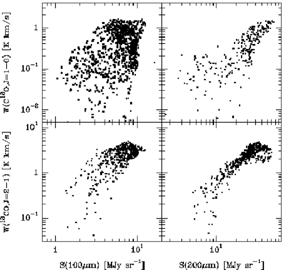
Figure 15: C¹⁸O(1–0) and ¹³CO(2–1) line areas as the function of 100$\mu$m and 200$\mu$m surface brightness. In plots containing the 200 $\mu$m surface brightness values the original data are smoothed to resolution of 100$\arcsec$. In the case of 100 $\mu$m the corresponding resolution is 70$\arcsec$

In Fig. 16, the C¹⁸O(1–0) column density (see Fig. 13 and Sect. 4) is compared with the dust optical depth at 200 $\mu$m. The figure confirms the good general correlation between the two. The C¹⁸O column density distribution may, however, be slightly more extended in the SE. This was already seen in the C¹⁸O(1–0) distribution. On the other hand, 200 $\mu$m optical depth is relatively larger immediately south of the (0,0) position.

Nevertheless, the linear relation does hold only at lower column densities. A linear least squares fit was made taking into account the uncertainty in both variables. For points with $\tau(200\mu$m)$<$5$\cdot$10^-3 we get

$$\frac{N({\rm C}^{18}{\rm O})}{10^{13}\,{\rm cm}^{-2}}=(4.62\pm 0.16)10^{4}\,\tau(200\mu{\rm m})-(1.5\pm 1.0).$$ (2)

Points at $\tau$(200$\mu$m)$<$5$\cdot$10^-5 were also discarded for this fit since the C¹⁸O column density estimates corresponding to these points are no longer reliable. When $\tau(200\mu$m) exceeds $\sim$5$\cdot$10^-3 the C¹⁸O column density is significantly below the prediction based on lower optical depths. The C¹⁸O emission could be reduced by depletion of gas phase molecules, a large drop in the excitation temperature towards the cold core or by the effect of optical depth.

5 CO depletion in the cloud core

The LTE analysis indicated C¹⁸O(1–0) optical depths below one. In the Monte Carlo model, the optical depth towards the cloud centre averaged over the telescope beam was 0.56. These results were based on the ¹³CO(1–0) and C¹⁸O(1–0) observations. Since the emission of the observed lines may come from different parts of the cloud, the determination of the optical depth remains uncertain to some extent. In the positions close to the cloud centre where C¹⁸O(2–1) was observed LTE analysis based on the two C¹⁸O lines gave somewhat higher estimates for the optical depth, $\tau\la$1.0. The optical depth is insufficient to cause any significant saturation of the C¹⁸O line and will not affect the accuracy of the column density estimates in Fig. 16.

Based on the LTE analysis, the excitation temperature was rather uniform over the cloud. Compared with other parts of the cloud the excitation temperature towards the cloud centre was lower by no more than 1 K. The column density estimates were based on an average value of 8.4 K. In Fig. 16, the vertical arrow indicates the change in the estimated column density if excitation temperature is reduced from a value 8.8 K to a value of 7.0 K. It is clear that even a drop of $\sim$2 K is insufficient to explain the relatively low C¹⁸O column density estimates at the position of high values of $\tau$(200$\mu$m).

The horizontal arrow in Fig. 16 indicates the shift in the value of $\tau(200\mu$m) when a value of optical depth is calculated with $T_{\rm dust}$=12.5 K instead of 12.0 K. Incorrect dust temperatures are, however, not likely to explain the relative drop of the C¹⁸O intensity. Firstly, the error should be $\sim$1 K or more at 12 K to bring the deviating points onto the fitted line even if the temperature were not changed outside the core. Errors in temperatures could be caused either by calibration or the background subtraction. If all 100 $\mu$m surface brightness values are multiplied by a constant, all $\tau(200\mu$m) estimates would be scaled with a factor that has very weak temperature dependence. An incorrect background subtraction, on the other hand, mostly affects the high temperatures which correspond to low surface brightness values. As an example, let us consider two dust temperatures, 12 K and 15 K. After the background subtraction, in L183 these typically correspond to 100 $\mu$m surface brightness values of 7 MJy sr^-1 and 3 MJy sr^-1. If we subtract 0.5 MJy sr^-1 from the 100 $\mu$m measurements the colour temperatures would drop to 11.85 K and 14.45 K and the corresponding 200 $\mu$m optical depth estimates would increase by 8% and 20%, respectively. The net change is only some 12% i.e. much less than the effect seen in Fig. 16.

Therefore, it seems that C¹⁸O depletion remains the most probable cause for the decreasing $N({\rm C^{18}O})/\tau(200\mu$m) ratio. In cloud cores the CO molecules freeze out onto the surfaces of the cold dust grains. Direct evidence of the process is provided by the observations of the molecular ice features (e.g. Tielens et al. tielens91 (1991)). As the result the properties of the dust grains are altered and this may explain some of the colour temperature variations observed in L183. In the centre of L183 the visual extinction exceeds 10^m and CO depletion has been detected in other clouds at similar extinction values. Kramer et al. (kramer99 (1999)) and Bergin et al. (bergin01 (2001)) have detected CO depletion in the cloud IC5146. In that cloud the relative C¹⁸O intensity decreases already below $A_{\rm V}$=10^m. Similarly in the cloud L977 a drop in C¹⁸O intensity attributed to depletion takes place at visual extinction $A_{\rm V}\sim 10^{\rm m}$ (Alves et al. alves99 (1999)). In L183 our models predicted central density close to $10^{5}$ cm^-3 for the spherical model with a radial density profile $\sim r^{-1.5}$. This density is probably exceeded in the cold core and e.g. in L1544 CO depletion was associated with densities above $10^{5}$ cm^-3 (Caselli et al. caselli99 (1998)).

Based on Fig. 16, the depletion factor is $\sim$1.5 in the centre of L183 where the dust temperature is close to 12 K. This is in perfect agreement with the findings of Kramer et al. (kramer99 (1999)) who have derived the depletion factor for IC5146 as a function of dust temperature.

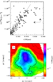
Figure 16: a) Correlation between the dust optical depth at 200 $\mu$m and the C¹⁸O column density derived from C¹⁸O(1–0) observations, assuming a constant excitation temperature of 8.4 K. The arrows indicate the shift if $N$(C¹⁸O) were calculated with a $\sim$2K lower excitation temperature, or if the optical depth were calculated using a 0.5 K higher dust temperature. The latter applies to the highest $\tau(200\mu$m) values corresponding to $T_{\rm dust}\sim$12 K. b) The distribution of the 200 $\mu$m optical depth over the area of highest optical depth. The dotted contour indicates the level $\tau(200\mu$m)=2$\cdot$10^-3. In (a) the points inside this contour are plotted with larger symbols. The solid contours show the distribution of the C¹⁸O column density. The highest contour is at 1.6$\cdot$10¹⁵ cm^-3 and the others are each a factor of two below the previous one.

6 DCO+ in the cold cloud core

H¹³CO+ and DCO+ are concentrated close to the 200$\mu$m maximum. The peaks of the intensity distributions of both species are very close to the position of the continuum source, within $\sim 2\arcmin$. While the 200$\mu$m emission continues to be strong towards the 100$\mu$m peak both H¹³CO+ and DCO+ are restricted to a narrow ridge running in the north-south direction. The distribution is therefore clearly different from either C¹⁸O or 200$\mu$m, although close to position (0,0) the 200$\mu$m emission is also elongated in the north-south direction. More importantly, no H¹³CO+ or DCO+ emission is seen close to the 100$\mu$m maximum, while the area of strong C¹⁸O emission covers also that position. At the position (4.5$\arcmin$, -2.5$\arcmin$) we get 2$\sigma$ upper limits of 0.10 K for H¹³CO+(1–0) and 0.20 K for DCO+(2–1) main beam temperature.

Fig. 17 shows the DCO+ distribution in relation to C¹⁸O. Both peak in the same region around position (0,0) and the small extension from this position towards the west can be interpreted to correspond to a similar feature seen in C¹⁸O. However, at the exact position of the DCO+ maximum, the C¹⁸O map shows a very slight depression, and in the south the two species are clearly anticorrelated, with stronger C¹⁸O emission seen on each side of the DCO+ ridge.

The 100 $\mu$m emission peaks some 5$\arcmin$ east of the DCO+ maximum and even in details the distribution is completely unrelated to the DCO+ emission. The correlation between DCO+ and 200 $\mu$m emission is not very good either. Both peak close to position (0,0) but compared with the FIR emission the DCO+ maximum is shifted one arcminute to the west. Apart from a similar shift the correlation is good north of the centre position. In the south the distributions of DCO+ and 200 $\mu$m are different. As already mentioned, no DCO+ emission was seen close to the eastern FIR peak. The DCO+ map does not quite extend to the southern 200 $\mu$m peak at position (1,-6) but between the northern and southern 200 $\mu$m peaks the DCO+ ridge goes over a region with relatively low FIR emission.

In Fig. 18a we compare the DCO+ distribution with the 200 $\mu$m optical depth. Due to the dust temperature gradient, $\tau(200\,\mu$m) is shifted relative to the 200 $\mu$m emission and coincides with the DCO+ distribution. Around position (0,0) and in the north, the correlation between $\tau(200\,\mu$m) and DCO+ is very good. In the south, the DCO+ follows roughly the dust optical depth distribution but the correlation is not perfect. The $\tau(200\,\mu$m) distribution is more extended SE of the centre position and the southern DCO+ peak at (1.5,  -4) lies just north of the third $\tau(200\,\mu$m) peak, i.e. it does not follow dust distribution. The southern part of the DCO+ ridge is outside the coldest dust core (Fig. 18b).

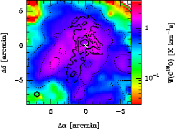
Figure 17: Contours of DCO+(2–1) integrated line area on the map of integrated C¹⁸O(1–0) line area. The DCO+ contours are at 0.2, 0.4, and 0.6 K km s^-1. The dotted contours indicate C¹⁸O(1–0) intensity levels from 0.5 to 2.0 K km s^-1 at intervals of 0.5 K km s^-1. The maps are presented at their original resolution. The beam sizes (46$\arcsec$ for C¹⁸O and 35$\arcsec$ for DCO+) are indicated with circles at the lower left corner.

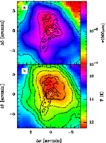
Figure 18: a) DCO+(2–1) contours on the map of 200 $\mu$m optical depth. The solid contours show the DCO+ distribution and are drawn at 0.2, 0.4, and 0.6 K km s^-1. The dotted contours indicate values 1$\cdot 10^{-3}$, 2$\cdot 10^{-3}$ and 4$\cdot 10^{-3}$ of 200 $\mu$m optical depth. b) DCO+(2–1) contours on the map of dust colour temperature. The solid DCO+ contours are drawn at 0.3, 0.5, 0.7 and 0.9 K km^-1. The dotted contours correspond to dust temperatures from 12 to 14 K at steps of 0.5 K. The maps are presented at their original resolution.

As the distributions of the DCO+ and H¹³CO+ are very similar, the same conclusions apply to the comparison of the H¹³CO+ distribution with CO species and FIR emission. At the position (0,0), the observed main beam temperatures are 1.5 K and 0.79 K for DCO+(2–1) and H¹³CO+(1–0) respectively. DCO+ seems to be more concentrated in this core, but the difference is not significant when the difference in the beam size is taken into account. In the upper panel of Fig. 19 the DCO+ and H¹³CO+ intensities are compared along the line going through the two cores. The DCO+ values were convolved to the resolution of the H¹³CO+ observations. In the main core, the H¹³CO+ is displaced to the north with respect to the DCO+. In the southern core, the relative intensity of H¹³CO+ is higher.

According to chemical models (Millar et al.millar89 (1989); Roberts & Millar roberts00 (2000)) the ratio between DCO+ and H¹³CO+ can be used as a tracer of gas temperature. The reaction

$$H_{3}^{+}+HD\leftrightarrow H_{2}D^{+}+H_{2}+\Delta E$$ (3)

is strongly temperature dependent. At low temperatures the production of $H_{2}D^{+}$ is enhanced and it reacts with CO to produce more DCO+. The abundance ratio also depends, however, on other factors such as cloud age, electron density and the total abundance of neutrals (Anderson et al. anderson99 (1999); Roberts & Millar roberts00 (2000)). This prevents the use of the ratio [DCO+]/[H¹³CO+] for direct temperature determination.

The observed change in the intensity of the DCO+ and H¹³CO+ lines indicates a higher gas temperature in the southern core. This is consistent with the difference in dust temperatures. Using the main beam antenna temperatures, the ratio of DCO+(2–1) and H¹³CO+(1–0) line areas increases from $\sim$1.0 in the south to $\sim$1.7 in the main core. The excitation states of DCO+ and H¹³CO+ should be very similar. The isothermal Monte Carlo model used to model the ¹³CO and C¹⁸O lines was used to predict DCO+ lines assuming an abundance of 5$\cdot$10^-11. Compared with the model in Sect. 4, the density needed to be increased almost a factor of two to produce lines $T_{\rm A}(J=1-0)\sim$ 0.8 K, in which case the line ratio was $T(1-0)/T(2-1)\sim$ 2. Assuming column density is directly proportional to observed intensity and using a value of 66 for the ratio ¹²C/¹³C (Langer & Penzias langer93 (1993)), we obtain values of 0.051 and 0.030 for the DCO+ to HCO+ abundance ratio in the two cores. The ratios indicate gas temperatures $\sim$10 K or less, depending on the set of reaction constants used (Millar et al.millar89 (1989); Roberts & Millar roberts00 (2000); see also Loren et al. loren90 (1990)). The difference between the northern and southern cores corresponds to a temperature change of at least 2 K.

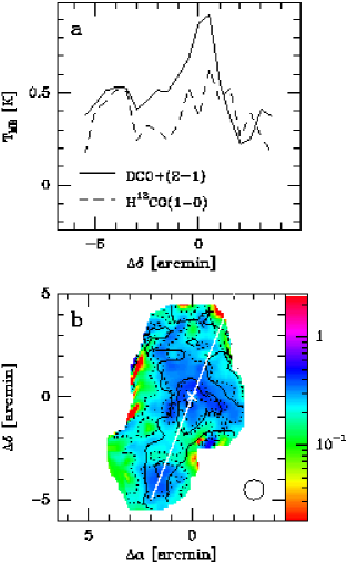
Figure 19: a) The DCO+(2–1) (solid line) and H¹³CO+(1–0) (dashed line) intensities along the line going through the two cores detected in these lines. b) DCO+(2–1) contours (solid lines) over-plotted on the H¹³CO+(1–0) map. The DCO+ contours levels are the same as in the previous figures. The dotted lines indicate H¹³CO+(1–0) values 0.2, 0.3 and 0.4 K km s^-1. The DCO+ data are convolved to the resolution of H¹³CO+ observations.

7 Comparison of optical extinction with FIR dust and CO column densities

In Fig. 20 we plot $A_{\rm R}$ as a function of $A_{\rm B}$, as derived from the starcounts (see Sect. 2.3). The dots denote individual extinction values obtained by averaging the counts in each grid point over a circle with radius 1.7$\arcmin$. In the averaging the weights were proportional to the area inside the circle which was, however, only slightly larger than original 2.8$\arcmin\times$2.8$\arcmin$ square used in the star counts.

We first calculated the average number of $R$-band stars in those 2.8$\arcmin\times$2.8$\arcmin$ squares with a given number of $B$-band stars. The average counts in these areas were transformed into extinction values. The relation with statistical errors is shown in Fig. 20 (dashed line). Linear least squares fit gives a relation $A_{\rm R}$ = (0.42 $\pm$ 0.02) $A_{\rm B}$. The fit takes into account uncertainty in both $A_{\rm B}$ and $A_{\rm R}$. If the intercept were included in the fit its value would be only $\sim 0.03$. If we calculate the average of the $A_{\rm R}$ values at all grid points with a given $A_{\rm B}$ (instead of first calculating the average number of stars) the derived relation becomes steeper, with a slope of 0.48$\pm$0.02. The value is still somewhat lower than the value $\sim$0.56 for the extinction law with $R_{\rm V}=A_{\rm B}/E_{\rm B-V}$=3.1. The fit is shown as a solid line in the figure. The least squares line fitted directly to ($A_{\rm B}$, $A_{\rm R}$) points gives also a slope of 0.48. Considering the possible systematic errors of $\sim$10% of our extinction values, due to uncertainties in the calibration of $logN(m)$ vs. $m$ slopes, our $A_{\rm R}/A_{\rm B}$ ratio is compatible with the standard reddening law ($R_{\rm V}=3.1$). On the other hand, it differs significantly from the value of $A_{\rm R}/A_{\rm B}$=0.66 valid for the case of $R_{\rm V}=5.0$ as derived for the “outer-cloud dust” (Mathis et al. mathis90 (1990)).

In the centre of L183 there were a few starcount squares where no stars were seen and for Fig. 20 the extinction was calculated using a value of 0.5 stars per square. The values, $A_{\rm R}\approx$5^m, still only represent a lower limit of the true extinction. In the most opaque area of 95 square arcminutes, four stars were detected in the $R$-band and this translates into an extinction of 5.3^m. In the $B$-band, no stars were seen in this area while a single star would correspond to an extinction of 6.8^m. Therefore, it is likely that at the very centre the extinction is at least $A_{\rm V}\sim$10^m.

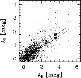
Figure 20: The relation between $B$-band and $R$-band extinction as derived from the starcounts. The lower points with errorbars are obtained by first averaging the $R$-band counts in areas with given number of $B$-band stars. The dashed line is the least squares line fitted to these. The upper points denote averages of $A_{\rm R}$ for given $A_{\rm B}$ and the dots correspond to star count averaged over circle with radius 1.7$\arcmin$. The solid line is the least squares fit to these points and has a slope of 0.48

Next $A_{\rm R}$ is compared with the hydrogen column density estimate derived from the C¹⁸O(1–0) observations (Fig. 13) and the 200 $\mu$m optical depth (Fig. 6). The data are convolved to the resolution $2.8\arcmin$ corresponding to the grid size used in the starcounts. The results are shown in Figs. 21 and 22.

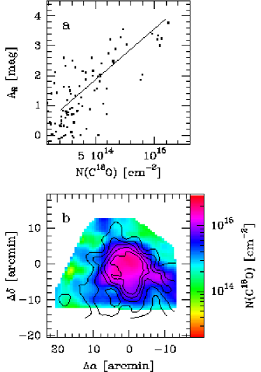
Figure 21: a) $R$-band extinction vs. C¹⁸O column density. b) $R$-band extinction contours drawn on the C¹⁸O column density map. The contours of extinction are drawn between 1^m and 5^m at intervals of 1^m. The C¹⁸O column densities have been convolved to the resolution of the extinction map, $\sim$2.8$\arcmin$.

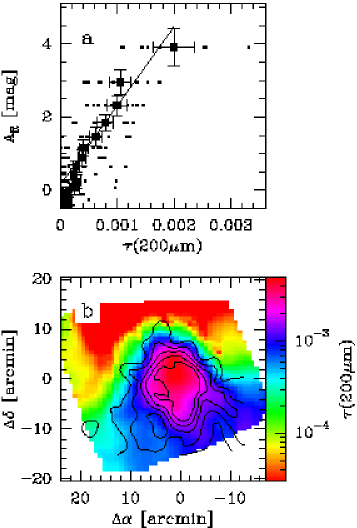
Figure 22: a) $R$-band extinction vs. 200 $\mu$m optical depth. b) $R$-band extinction contours on the map of $\tau$(200$\mu$m) which has been convolved to a resolution of 2.8$\arcmin$. The extinction contours are drawn between 1^m and 5^m at intervals of 1^m.

The C¹⁸O column density and the extinction are clearly correlated. The C¹⁸O depletion seen in Fig. 16 is not visible, however, as the centre region where no $R$-band stars were detected is not included in the figure. This limits the dynamical range available. Furthermore, at low column densities the noise increases rapidly due to the decreasing signal-to-noise ratio of the C¹⁸O spectra. The maximum extinction corresponding to one star per grid pixel area was $\sim$4^m. For the plot the star counts were again averaged over a circle with radius 1.7$\arcmin$ but points with $A_{\rm R}>$4^m are omitted in the figure. The least squares line is

$$A_{\rm R}/{\rm mag}=(3.4\pm 0.2)10^{-15}N({\rm C}^{18}\rm{O})+(0.1\pm 0.1).$$ (4)

With the earlier relation between $A_{\rm R}$ and $A_{\rm B}$ and the assumed value of $R$=3.1 this translates to $N$(C¹⁸O)/cm^-2=1.9$\cdot$10¹⁴A_V-4$\cdot$10¹³. The slope is similar to the value found in regions of high extinction in Taurus and Ophiuchus by Frerking et al. (frerking82 (1982)) but steeper than the corresponding value for the lower range $2^{\rm m}<A_{\rm V}<4^{\rm m}$ where the value in Taurus was 0.7$\cdot$10¹⁴ cm^-2 mag^-1. The slopes determined in L977 and IC5146 for $A_{\rm V}\la$10^m (Alves et al. alves99 (1999)) are rather similar, $\sim$2$\cdot$10¹⁴ cm^-2 mag^-1. Also Harjunpää et al. (harjunpaa96 (1996)) found a similar slope in Corona Australis while in the Coalsack the value was only $\sim$1.2$\cdot$10¹⁴ cm^-2 mag^-1. Note that if we assume standard extinction (Rieke & Lebofsky rieke85 (1985)) to transform $A_{\rm R}$ directly to $A_{\rm V}$ our slope increases to 2.2$\cdot$10¹⁴ cm^-2 mag^-1.

Within the statistical uncertainty of the starcounts, the extinction map agrees well with $\tau$(200$\mu$m). The dots in Fig. 22 correspond to the star counts on the original grid. The filled squares with error bars are averages for each discrete value of $A_{\rm R}$. The least squares line based on the interval $1.0^{\rm m}<A_{\rm R}<4.0^{\rm m}$ is

$$A_{\rm R}/{\rm mag}=(2.2\pm 0.3)10^{3}\tau(200\mu{\rm m})+(0.2\pm 0.2).$$ (5)

The relation can be used to derive an extrapolated extinction value for the centre region where no stars were detected. In the centre there are several 200 $\mu$m pixels with $\tau(200\mu{\rm m})\sim 6\cdot 10^{-3}$. According to the previous relation, this corresponds to extinction $A_{\rm R}\approx 13^{\rm m}$ and visual extinction of the order of 17^m. This clearly exceeds the previous estimates, and is based on the sharp increase of the 200 $\mu$m optical depth in the cold cloud core.

Assuming a standard extinction law ($R_{\rm V}$=3.1) between $V$- and $R$-bands, from Eq. 5 we obtain $\tau(200\mu{\rm m})/A_{\rm V}=3.4\cdot 10^{-4}$ mag^-1. For the cloud centre, the ratio increases to 3.8$\cdot 10^{-4}$ mag^-1 but is still below the value of 5.3$\cdot 10^{-4}$mag^-1 found in the Thumbprint Nebula (Lehtinen et al. lehtinen98 (1998)). In L183, the comparison between 100 $\mu$m optical depth and visual extinction gives a ratio 2.1$\cdot 10^{-3}$mag^-1 which is similar to the value in the Thumbprint Nebula.

For a value of $\tau(200\mu{\rm m})=1.0\cdot 10^{-3}$, the previous relations between $\tau(200\mu$m) and $A_{\rm R}$ and between $A_{\rm R}$ and C¹⁸O column density predict a column density of N(C¹⁸O)=6.6$\cdot 10^{14}$ cm^-2. Directly using the relation between $\tau(200\mu$m) and N(C¹⁸O) (Eq. 2) we would obtain a lower value, 4.5$\cdot 10^{14}$ cm^-2. One must remember, however, that Eq. 2 was determined over a much larger range of optical depths and consequently that relation may already be affected by the C¹⁸O depletion.

8 Conclusions

The main conclusions drawn from the comparison of far-infrared data and molecular line observations in L183 are:

• The 100 $\mu$m and 200 $\mu$m emission clearly have different distributions.

• The 200 $\mu$m maximum indicates the position of a core where either the dust temperature becomes very low or the dust properties have changed. The colour temperature determined from the 100 $\mu$m and 200 $\mu$m observations with an emissivity law of $\nu^{2}$ is $\la$12 K. The dust optical depth peaks at the same position.

• Of the molecular lines, the optically thin C¹⁸O best traces the dust distribution. Although better correlated with the 200 $\mu$m surface brightness it shows strong emission at the locations of both the 100 $\mu$m and 200 $\mu$m maxima. The optically thick ¹²CO and ¹³CO lines peak south of the dust cores.

• C¹⁸O is depleted in the cloud centre. The depletion factor is $\sim$1.5 in the core where dust temperature is close to 12 K.

• Relative to each other, the DCO+ and H¹³CO+ lines show very similar distributions. Their distribution is completely different from any of the observed CO lines but a good correlation does exist with the 200 $\mu$m optical depth.

• The estimated mass within 10$\arcmin$ of the (0,0) position was 25 $M_{\sun}$, based on the 200 $\mu$m optical depths and $\sim$40 $M_{\sun}$ based on the C¹⁸O column densities.

• The 100 $\mu$m surface brightness is not well correlated with the extinction. A linear relation does exist between $A_{\rm R}$ and dust optical depth at 200 $\mu$m. Based on this correlation we derive for the cloud centre an extinction $A_{\rm V}\sim 17^{\rm m}$.

- (1) Alves J., Lada C.J., Lada E.A. 1999, ApJ 515, 265
- (2) Anderson I.M., Caselli P., Haikala L.K., Harju J. 1999, A&A 347, 983
- (3) Bahcall J.N., Ratnatunga K.U., Buser R., Fenkart R.P., Spaenhauer A., 1985, ApJ 299, 616
- (4) Bahcall J.N., Soneira R.M. 1980, ApJS 44, 73
- (5) Becker W., Fenkart R. 1976, Photometric Catalogue of Stars in Selected Areas and other Fields in the RGU-System, Vol. 1, Basel: Astron. Inst. Univ. Basel
- (6) Bergin E.A., Ciardi D.R., Lada C.J., Alves J., Lada E.A. 2001, ApJ (submitted), astro-ph 0103521
- (7) Bergin E.A., Langer W.D., Goldsmith P.F., 1995, ApJ 441, 222
- (8) Bergin E.A., Snell R.L., Goldsmith, P. F. 1996, ApJ 460, 343
- (9) Bernard, J.-P., Abergel A., Ristorcelli I., Pajot F., Boulanger F. et al. 1999, A&A 347, 640
- (10) Bettens R.P.A, Lee H.-H., Herbst E., 1995, ApJ 443, 664
- (11) Bohlin R.C., Savage B.D., Drake J.F., 1978, ApJ 224, 132
- (12) Bok B.J. 1956, AJ 61, 309
- (13) Boulanger F., Abergel A., Bernard J.P., et al., 1996, A&A 312, 256
- (14) Cambrésy L, Boulanger F., Lagache G., Stepnik B. 2001, A&A (submitted), astro-ph 0106507
- (15) Caselli P., Walmsley C.M., Tafalla M., Dore L., Myers P.C. 1999, ApJ 532, L165
- (16) Caselli P., Walmsley C.M., Terzieva R., Herbst E., 1998, ApJ 499, 234
- (17) Clark F.O., Laureijs R.J., Prusti T., 1991, ApJ 371, 602
- (18) Désert F.-X., Boulanger F., Puget J. L., 1990, A&A 237, 215
- (19) Dickens J.E., Irvine W.M., Snell R.L., et al., 2000, ApJ 542, 870
- (20) Franco G., 1989, A&A 223, 313
- (21) Frerking M.A., Langer W.D., Wilson R.W. 1982, ApJ 262, 590
- (22) García-Lario P. 2000, 2nd post-operations cross-calibration report v. 1.0, http://www.iso.vilspa.esa.es/users/expl_lib/ ISO/2nd_status_report_ext.ps.gz
- (23) Gibb A.G., Little L.T., 1998, MNRAS 295, 299
- (24) Guélin M., Langer W.D., Wilson R.W., 1982, A&A 107, 107
- (25) Guélin M., Langer W.D., Snell R.L., Wootten H.A., 1977, ApJ 217, L165
- (26) Harjunpää P., Mattila K. 1996, A&A 305, 920
- (27) Herbst E., Leung C.M., 1989, ApJS 69, 271
- (28) Herbst E., Leung C.M., 1990, A&A 233, 177
- (29) Juvela M. 1997, A&A 322, 943
- (30) Kessler M.F., Steinz J.A., Anderegg M.E. et al., 1996, A&A 315, L27
- (31) Kramer C., Alves J., Lada C.J., Lada E.A., Sievers A., Ungerechts H., Walmsley C.M. 1999, A&A 342, 257
- (32) Laureijs R.J., Clark F.O., Prusti T., 1991, ApJ 372, 185
- (33) Laureijs R. J., Fukui Y., Helou, G. et al., 1995, ApJS 101, 87
- (34) Laureijs R.J., Haikala L., Burgdorf M. et al., 1996, A&A 315, L317
- (35) Lee H.-H., Bettens R.P.A., Herbst E., 1996, A&AS 119, 111
- (36) Lehtinen K., Lemke D., Mattila K., Haikala L. K. 1998, A&A 333, 702
- (37) Lehtinen et al., 2000, in D. Lemke, M. Stickel, K. Wilke (eds.), ISO Surveys of a Dusty Universe, Lecture Notes in Physics, Springer, p. 317
- (38) Lee H.-H., Herbst E., Pineau Des Forets G., et al., 1996, A&A 311, 690
- (39) Lemke D., Klaas U., Abolins J., et al. 1996, A&A 315, L64
- (40) Langer W.D., Penzias A.A. 1993, ApJ 408, 539
- (41) Leung C.M., Herbst E., Huebner W.F. 1984, ApJS 56, 231
- (42) Liljeström T. 1991, A&A 244, 483
- (43) Loren R.B., Wootten A., Wilking B.A. 1990, ApJ 365, 269
- (44) Mathis J.S. 1990, ARAA 28, 37
- (45) Mattila K. 1979, A&A 78, 253
- (46) Meny C., Serra G., Lamarre J. M., Ristorcelli I, Bernard J. P., Giard M., Pajot F., Stepnik B., Torre, J. P. 2000, ESA-SP 455, 105
- (47) Millar T.J., Bennett A., Herbst E. 1989, ApJ 340, 906
- (48) Millar T.J., Farquhar P.R.A., Willacy K., 1996, A&AS 121, 139
- (49) Ossenkopf V. 1993, ApJ 280, 617
- (50) Padoan P., Juvela M., Bally J., Nordlund , 2000, ApJ 529, 259-267
- (51) Pratap P., Dickens J.E., Snell R.L., et al., 1997, ApJ 486, 862
- (52) van Rhijn, P.J. 1929, Publ. Astron. Lab. Groningen No. 43
- (53) Rieke G.H., Lebofsky M.J. 1985, ApJ 288, 618
- (54) Roberts H., Millar T.J. 2000, A&A 361, 388
- (55) Snell R.L., 1981, ApJS 45, 121
- (56) Snell R. L., Schloerb F. P., Young J. S. et al. 1981, ApJ 244, 45
- (57) Snyder L.E., Hollis J.M., Buhl D., Watson W.D., 1977, ApJL 218, 61
- (58) Stahler S. W., 1984, ApJ 281, 209
- (59) Stark R., Wesselius P.R., van Dishoeck E.F., Laureijs R.J., 1996, A&A 311, 282
- (60) Stepnik B., Abergel A., Bernard J.-P., Boulanger F., Cambrésy L. et al. 2001, A&A, in press
- (61) Swade D.A., 1989, ApJS 71, 219
- (62) Swade D.A., 1989, ApJ 345, 828
- (63) Swade, D.A., Schloerb F.P., 1992, ApJ 392, 543
- (64) Tielens A., Tokunaga A., Geballe T., Baas F. 1991, ApJ 381, 181
- (65) Turner B.E., Terzieva R., Herbst Eric, 1999, ApJ 518, 699
- (66) Turner B.E., Herbst E., Terzieva R., 2000, ApJS 126, 427
- (67) Ungerechts H., Walmsley C. M., Winnewisser G., 1980, A&A 88, 259
- (68) Ward-Thompson D., Scott P.F., Hills R.E., 1994, MNRAS 268, 276
- (69) Ward-Thompson D., Kirk J.M., Crutcher R.M., et al., 2000, ApJ 537, 135
- (70) Warin S., Benayoun J.J., Viala Y.P., 1996, A&A 308, 535
- (71) Watson W.D., Snyder L.E., Hollis J.M., 1978, ApJ 222, L145
- (72) Wright E.L. 1987, ApJ 320, 818
- (73) Wootten A., Loren R.B., Snell R.L., 1982, ApJ 255, 160
- (74) Wootten A., Loren R.B., 1987, ApJ 317, 220