Spectra of the Expansion Stage of X-Ray Bursts

Abstract

We present an analytical theory of thermonuclear X-ray burst atmosphere structure. Newtonian gravity and diffusion approximation are assumed. Hydrodynamic and thermodynamic profiles are obtained as a numerical solution of the Cauchy problem for the first-order ordinary differential equation. We further elaborate a combined approach to the radiative transfer problem which yields the spectrum of the expansion stage of X-ray bursts in analytical form where Comptonization and free-free absorption-emission processes are accounted for and $\tau\sim r^{-2}$ opacity dependence is assumed. Relaxation method on an energy opacity grid is used to simulate radiative diffusion process in order to match analytical form of spectrum, which contains free parameter, to energy axis. Numerical and analytical results show high similarity. All spectra consist of a power-law soft component and diluted black-body hard tail. We derive simple approximation formulae usable for mass-radius determination by observational spectra fitting.

1 Introduction

First discovered by Grindlay et al. (1975), strong X-ray bursts are believed to occur due to thermonuclear explosions in the bottom helium-reach layers of the atmosphere accumulated by a neutron star during the accretion process in close binary system. Since then dozens of burster-type X-ray sources were found. One of the distinctive feature of Type I X-ray bursts is the sudden and abrupt ($\sim 1$ s) luminosity increase (expansion stage) followed by exponential decay (contraction stage). Energy released in X-ray radiation during the first seconds greatly exceeds the Eddington limit for layers above the helium burning zone which are no longer dynamically stable. Super-critically irradiated shells of atmosphere start to move outward, producing an expanding wind-like envelope. The average lifetime of an X-ray bursts is sufficient for steady-state regime of mass loss to be established when the local luminosity throughout the most of the atmosphere is equal or slightly greater than the Eddington limit.

During the last two decades the problem of determining properties of radiatively driven winds during X-ray bursts was subjected to extensive theoretical and numerical studies. Various theories were put forward with gradually increasing level of accuracy of the problem description, but only a few approaches addressed the case of considerably expanded photosphere under influence of near-Eddington luminosities (London et al., 1986; Ebisuzaki, 1987; Lapidus, 1991; Titarchuk, 1994). See Lewin, Paradijs & Taam (1993) for a detailed review of X-ray burst study during 80’s and the beginning of 90’s.

Similarly to the problem of accretion flows, notion of the existence of sonic point in continuous flow became a natural starting point in the analysis of wind flows from stellar objects. Ebisuzaki al. (1983), hereafter EHS, investigated the structure of the envelopes with steady-state mass outflow and pointed out the higher Eddington luminosity in the inner shells due to the prevalent higher temperatures and correspondingly lower Compton scattering opacities. They showed that the product of opacity and luminosity remains almost constant throughout the atmosphere which is the key assumption of the model. The existence of wind-like solutions for critically irradiated atmospheres was proved. Titarchuk (1994), hereafter T94, studied analytically spectral shapes of the expansion and contraction stages of bursts. He showed how EHS’s approach to hydrodynamic problem can be greatly simplified with the sonic point condition properly calculated and tied with conditions at the bottom of the envelope. Haberl & Titarchuk (1995) applied the T94 model to extract the neutron star mass-radius relations from the observed burst spectra in 4U 1820-30 and 4U 1705-44.

Nobili et al. (1994), hereafter NTL, adopted a high accuracy numerical approach to the problem of X-ray burster atmosphere structure based on the moment formalism (Thorne, 1981; Nobili,Turolla & Zamperi., 1991). They integrated a self-consistent system of frequency-independent, relativistic, hydrodynamical and radiative transfer equations over the whole atmosphere including the inner dense helium-burning shells. Three important characteristic of X-ray burst outflow were obtained in this work: the helium-burning zone temperature was maintained approximately at the level of $3\times 10^{9}$ K, the temperature of the photosphere was shown to depart appreciably from the electron temperature and to stay constant at the outer shells, and the existence of the maximum and the minimum values of the mass loss rate was found.

One of the goals of these studies was to provide the algorithm of determination of the compact object characteristics by analyzing observational data. With the advent of high spectral and time resolution observational instruments (such as Chandra, RXTE, USA, XMM-Newton missions) the task of obtaining a suitable tool for fitting the energy spectra became extremely important. Despite numerous earlier studies of X-ray burst observations, recent developments have shown a growing interest of the astrophysical community in this area (Strohmayer & Brown, 2001; Kuulkers et al., 2001).

Obviously, the problem of radiative transfer in relativistically moving media is very complicated one and under rigorous consideration it must be solved numerically. In this paper we develop an alternative approach which allows both numerical and analytical solutions and successfully accounts for all crucial physical processes involved. We show how this problem under some appropriate approximations yields the spectrum of radiation from spherically symmetric outflows in an analytical form. We concentrate on the case of extended atmosphere with inverse cubic power dependence of the number density on radius, which is more appropriate for the expansion stage but can also be employed for description of the contraction as a sequence of models with decreasing mass-loss rate.

We represent a numerical approach to the problem which then provides the validation of our analytical description. We adopt the general approach formulated in EHS and developed in T94. The problem of determining profiles of thermodynamic variables of steady-state radiatively driven outflow was solved in T94. The problem is reduced to the form of a first order differential equation, which allows easy and precise numerical solution. For a completeness we present this method in Section 2. Using atmospheric profiles obtained for different neutron star configurations we solve the problem of radiative transfer by relaxation method on an energy-opacity logarithmic grid. We perform temperature profile correction by applying temperature equation to the obtained spectral profiles. The basic formulae are given in Section 3.1. Then the analytical description of the problem is represented in detail. The analytic solution of radiative transfer equation on the atmospheric profile $\tau\sim r^{-2}$ is presented in T94. Here we review the solution by carrying out the integration without introducing any approximations. In Section 4 we compare and match our analytical and numerical results to describe the behavior of free parameter. We finalize our work by examining the properties of our analytic solution, combine it with the results of Section 4 and construct the final formula for fitting the spectra in Section 5. The discussion of our method along with some other important issues concerning the problem being solved are presented in Section 6. Conclusions follow in the last Section.

2 Hydrodynamics

As we already mentioned, that the calculation of X-ray burst spectra can be treated as a steady state problem. To justify this assumption one has to compare the characteristic times of phenomena considered. Time scale for the photosphere to collapse can be estimated as follows

$$t_{coll}=\int_{r_{s}}^{r_{ph}}\frac{dr}{v_{coll}},\quad\mathrm{where}\quad v_{coll}\approx\sqrt{\frac{2\,GM_{ns}}{r}(1-l)}.$$

Here $r_{s}$ denotes the sonic point radius, which is adopted as the outer boundary of the photosphere throughout this paper. Dimensionless luminosity is $l=L/L_{Edd}$, where Eddington luminosity is given by

$$L_{Edd}=\frac{4\pi c\,GM_{ns}}{\kappa}.$$ (1)

Opacity $\kappa$ is expressed by the Compton scattering opacity with Klein-Nishina correction by (Paczynski, 1983)

$$\kappa=\frac{\kappa_{0}}{(1+\alpha T)},$$ (2)

$\kappa_{0}=0.2(2-Y_{He})~{}{\rm cm}^{2}g^{-1}$ with $Y_{He}$ being the helium abundance, and $\alpha=2.2\times 10^{-9}K^{-1}$. It is exactly this temperature dependence of the opacity that is responsible for the excessive radiation flux, which appears to be super-Eddington to the outer less hot layers of the atmosphere. In the framework of strong X-ray bursts the following condition are usually satisfied: $r_{s}\gtrsim 10^{3}$km $>>r_{ph}$ , $l\sim 0.99$. Putting $m=M_{ns}/M_{Sun}\sim 1$ results in a time of collapse of the order of several seconds, the observed time which a Type I X-ray burst usually lasts. For evaluation of the time for photons to diffuse through the photosphere, we note that a number of scattering events is $N\approx\tau_{ph}^{2}$ [see, for example, Rybicki & Lightman (1979)], where $\tau_{ph}$ is the total opacity of the photosphere, which is $\sim 10$. The time for a photon to escape is

$$t_{esc}\sim\frac{\tau_{ph}^{2}}{\sigma_{T}n_{e}c}\sim\frac{r_{ph}}{c}\tau_{ph}\sim 0.1~{}~{}s.$$

This indicates that the hydrodynamic structure develops at least ten times slower than the photons diffusing time through the photosphere. Although these time scales can become comparable in cases of greatly extended atmospheres, generally steady-state approximation is acceptable.

2.1 Basic equations for radiatively driven outflow

The problem of mass loss as a result of radiatively driven wind was formulated by EHS. For convenience of the reader we summarize all equations important for the derivations in the following sections and refer the reader to EHS paper for details. The system of equations describing steady-state outflow in spherical symmetry consists of a well known Euler (radial momentum conservation) equation

$$v\frac{dv}{dr}+\frac{GM}{r^{2}}+\frac{1}{\rho}\frac{dP}{dr}=0,$$ (3)

the mass conservation law

$$\frac{d}{dr}(4\pi r^{2}\rho v)=0,$$ (4)

the averaged radiation transport equation in the diffusion approximation

$$\kappa L_{r}=-\frac{16\pi acr^{2}T^{3}}{3\rho}\frac{dT}{dr},$$ (5)

and the entropy equation

$$vT\frac{ds}{dr}+\frac{1}{4\pi r^{2}\rho}\frac{dL_{r}}{dr}=0,$$ (6)

where $P,\rho,T,s$ and $L_{r}$ are, respectively, the pressure, the density, the temperature, the specific entropy, and the diffusive energy flux flowing through a shell at $r$.

The outflowing gas is taken to be ideal. Dimensionless coordinate $y$, which is the ratio of the radiation pressure $P_{r}$, to the gas pressure $P_{g}$, is introduced by

$$y=\frac{P_{r}}{P_{g}}=\frac{\mu m_{p}}{k}\frac{aT^{3}/3}{\rho},$$ (7)

where $\mu=4/(8-5Y_{He})$ and $m_{p}$ are the mean molecular weight and the mass of proton, respectively. Then the other thermodynamic quantities are expressed in terms of $y$ and $T$ as

$$P=P_{r}+P_{g}=\left(1+\frac{1}{y}\right)\frac{aT^{4}}{3},$$ (8)

$$\rho=\frac{a\mu m_{p}}{3k}\frac{T^{3}}{y},$$ (9)

$$s=\left(\frac{k}{\mu m_{p}}\right)[4y+\ln y-(3/2)\ln T],$$ (10)

$$h=\frac{k}{\mu m_{p}}(4y+5/2)T,$$ (11)

where $h$ is the specific enthalpy.

Integrals of equation (4) and (3) give energy flow and mass flux correspondingly

$$4\pi r^{2}\rho v=\Phi,$$ (12)

$$\left(\frac{v^{2}}{2}-\frac{GM}{r}+h\right)\Phi+L_{r}=\Psi.$$ (13)

To make two more integrations, which can not be performed analytically, the constancy of $\kappa L_{r}$, which stands for the integral of equation (5), over the relevant layers is assumed. In EHS this assumption is confirmed numerically. We can also justified by the following consideration. At the near-Eddington regime the radiation pressure $aT^{4}/3$ is much greater than the pressure of gas almost everywhere except for the innermost layers adjacent to the helium-burning zone. Neglecting the gas pressure in equation (3) and multiplying it by $-r^{2}$ we get

$$\frac{\kappa L_{r}}{4\pi c}=GM+r^{2}v\frac{dv}{dr}.$$ (14)

Here we moved first two terms of (3) to the right hand side and used equation (5) to express third term by $\kappa L_{r}$. For inner and intermediate layers of the atmosphere the last term in (14) is negligible and equation reduces to $\kappa L_{r}=\kappa_{0}L_{0}$. This term can become considerably large for the outermost layers where $L_{r}$ must exceed $L_{Edd}$. This also is in agreement with observations of X-ray bursts from which super-Eddington luminosities are inferred. For the sake of analytical consideration we consider $\kappa L_{r}$ to be constant throughout the whole atmosphere, and the third integral is

$$\kappa L_{r}=\kappa_{0}L_{0}=const.$$ (15)

Replacing $L_{r}$ of equation (6) with equation (15), the fourth integral is obtained as

$$\Phi s+\alpha L_{0}\ln T=\Xi=const.$$ (16)

Boundary conditions need to be imposed at the bottom and the outer boundary to determine the four integration constants $\Phi,\Psi,L_{0}$, $\Xi$ and to obtain a specific solution.

At the bottom of the atmosphere close to the helium-burning zone there should be a point where gas and radiation pressure are equal. As another important numerical result EHS showed that near the neutron star surface the temperature and radius profiles level off with respect to $y$, so there is always a point where

$$r=r_{b},~{}T=T_{b},~{}y=1,$$ (17)

and $r_{b}$ is well approximated by the radius of the neutron star $R_{ns}$. However, $T_{b}$ can not be considered as a real temperature of helium-burning shell at the bottom of the star surface because thermonuclear processes are not included in the model. Rigorous account of helium-burning NTL shows that temperature of burning shells vary in small range of values.

To obtain the outer boundary condition the concept of sonic point is used. For the solution to be steady-state and to have finite terminal velocity it should pass sonic point where

$$v_{s}^{2}=\frac{GM_{ns}}{2r_{s}}=\left(\frac{\partial P_{s}}{\partial\rho_{s}}\right)_{\Xi}=\left(\frac{k}{\mu m_{p}}\right)Y_{s}T_{s},$$ (18)

$$Y_{s}=\frac{\lambda+4(1+y_{s})(1+4y_{s})}{\lambda+3(1+4y_{s})},$$ (19)

where $\lambda$ is a quantity related to the ratio of the energy flux to the mass flux (see formula 22, below). In EHS this formula contains a typo. We give a proper derivation of this form for $Y_{s}$ in Appendix C.

2.2 ODE solution of the hydrodynamic problem

T94 has shown how the treatment of the hydrodynamic problem can be reduced to a Cauchy problem with the boundary condition determined at the sonic point. This treatment provides a high-accuracy method of obtaining the hydrodynamic solution. The crucial point is to relate the position of the sonic point with the values of the velocity and the thermodynamic quantities before solving the set of appropriate hydrodynamic equations. The profile of the expanded envelope is then obtained as a result of the integration of a single first-order ordinary differential equation (ODE) from the sonic point inward up to the neutron star surface. For completeness we present the details of this approach.

At the bottom of the atmosphere the potential energy per unit mass of the gas, $GM/r$, is significantly greater than the kinetic energy, $v^{2}/2$, and enthalpy. Therefore, by ignoring these terms in equation (13), we obtain the value of the mass flux

$$\Phi=\frac{R_{ns}}{GM_{ns}}\alpha T_{b}L^{0}_{Edd}.$$ (20)

The inner boundary condition (17), the integral (16), and equation (10) for entropy can be used to find the temperature distribution with respect to $y$

$$T=T_{b}\,y^{-1/\lambda}\exp\left[-\frac{4(y-1)}{\lambda}\right],$$ (21)

and

$$\lambda=\frac{\alpha\mu m_{p}}{k\Phi}L_{0}-\frac{3}{2}.$$ (22)

The condition at the sonic point (18) allows us to find the constant $\Psi$

$$\Psi=h_{s}\Phi+L_{r}(r_{s})-\frac{3}{4}\frac{GM}{r_{s}}\Phi.$$ (23)

Combining the mass and energy conservation laws (12) and (13), the specific enthalpy and density equations (9) and (11) and eliminating the radial coordinate $r$ between equations (12) and (13) yield the following dependence of the velocity derivative $v^{\prime}$ with respect to $y$

$$v^{\prime}_{y}(y,v)=v\left[\left(1+3\frac{1+4y}{\lambda}\right)\frac{1}{y}-75.2\frac{rT(8-5Y_{He})(1+4y)(1+\alpha T)}{\lambda r_{b,6}T_{b,9}(\Psi/\Phi-v^{2}/2-h+GM_{ns}/r)}\right].$$ (24)

Derivation of equation (24) is given in Appendix D.

By imposing boundary conditions at the bottom of the extended envelope (at the neutron star surface) and at the sonic point, we can determine the four integration constants necessary to obtain a specific solution. One can note the obvious fact that the bottom of the envelope can not serve as a starting point of integration of equation (24) as long as $v_{b}=0$, which introduces uncertainty. Fortunately, we can calculate parameters at the sonic point in the framework of our problem description by solving a nonlinear algebraic equation, which involves only $y_{s}$, the ratio of the radiation pressure $P_{r}$ to the gas pressure $P_{g}$ at that point. Substitution of the radial coordinate $r_{s}$ and velocity $v_{s}$ from the definition of the sonic point position (18), and the sonic point density, $\rho_{s}$ from equation (9), we find

$$r_{s}=\frac{GM_{ns}\,\mu m_{p}}{2kY_{s}T_{s}},\hskip 7.22743ptv_{s}=\left(\frac{k}{\mu m_{p}}Y_{s}T_{s}\right)^{\frac{1}{2}},\hskip 7.22743pt\rho_{s}=\frac{a\mu m_{p}}{3k}\frac{T_{s}^{3}}{y_{s}},$$

and the expression for the temperature given in equation (21) into the mass conservation law (12), after some algebra give an equation for the value of $y_{s}$

$$y_{s}=\frac{\lambda}{4}\ln\left\{\left[\frac{(2-Y_{He})m^{2}}{r_{b,6}T_{b,9}}\right]^{2/3}\frac{T_{b}}{0.149\,(8-5Y_{He})^{5/3}Y_{s}y_{s}^{1/\lambda+2/3}}\right\}+1.$$ (25)

Here $r_{b,6}$ and $T_{b,9}$ are the neutron star surface radius and temperature in units of $10^{6}$ cm and $10^{9}$ Kelvin respectively. Since $Y_{s}$ is expressed in terms of $y_{s}$ (eq. 19), equation (25) can be solved to determine the value of $y_{s}$. Knowledge of $y_{s}$ can then, by substitution in equation (21), yield the value of the temperature at the sonic point $T_{s}$ and then $v_{s}$ from equation (18). It is now possible to relate $v_{s}$ to $T_{s}$, $T_{b}$, $r_{s}$, $r_{b}$, thus obtaining the analytical expression for the various dynamical quantities at the sonic point in terms of the values of the parameters associated with the boundary conditions. To obtain the solution of the hydrodynamical problem for a particular set of input parameters we use a standard Matlab/Octave package function minimizators and ODE solvers.

3 Radiative Transfer Problem

The radiation field of X-ray burst atmosphere may be described by the diffusion equation, written in spherical geometry, with the Kompaneets’s energy operator (see T94):

$$\frac{1}{3}\left(\frac{\partial^{2}J_{\nu}}{\partial\tau^{2}}-\frac{2}{r\alpha_{T}}\frac{\partial J_{\nu}}{\partial\tau}\right)=\frac{\alpha_{ff}}{\alpha_{T}}(J_{\nu}-B_{\nu})-$$

$$\hskip 28.90755pt-\frac{kT_{e}}{m_{e}c^{2}}\,x_{0}\frac{\partial}{\partial x_{0}}\left(x_{0}\frac{\partial J_{\nu}}{\partial x_{0}}-3J_{\nu}+\frac{T_{0}}{T}J_{\nu}\right),$$ (26)

where $x_{0}=h\nu/kT_{0}$ is a dimensionless frequency, $T_{0}$ being the effective temperature; $\alpha_{ff}$ and $\alpha_{T}=\sigma_{T}n_{e}$ are the coefficients of free-free absorption and Thompson scattering, respectively, whose ratio is given by (Rybicki & Lightman, 1979)

$$\frac{\alpha_{ff}}{\alpha_{T}}=1.23\,\rho g_{14}^{7/8}(1-Y_{He}/2)^{7/8}\Psi(x_{0})\left(\frac{T_{0}}{T}\right)^{1/2}$$ (27)

with

$$\Psi(x_{0})=\frac{\tilde{g}(x_{0}T_{0}/T)}{x_{0}^{3}}\left(1-e^{-x_{0}T_{0}/T}\right).$$

Here $\tilde{g}(x)$ is the Gaunt factor (Greene, 1959)

$$\tilde{g}(x)=\frac{\sqrt{3}}{\pi}\,e^{x/2}K_{0}(x/2),$$

$K_{0}(x)$ is the Macdonald function, and $g_{14}$ denotes the free-fall acceleration onto the neutron star surface, in units of $10^{14}$ cm s^-1.

We combine equation (26) with the outer boundary condition of zero energy inflow

$$\left(\frac{\partial J_{\nu}}{\partial\tau}-\frac{3}{2}J_{\nu}\right)\Bigl{|}_{\tau=0}=0$$ (28)

and the condition of equilibrium blackbody spectrum at the bottom of the photosphere, which is represented in a dimensionless form as

$$B_{\nu}=\frac{x_{0}^{3}}{\exp(x_{0}T_{0}/T)-1}.$$ (29)

We will make use of the temperature equation, which is obtained by integration of (26) over frequency. The opacity operator vanishes as a result of the total flux conservation with respect to optical depth, leaving us with

$$\frac{kT_{e}}{mc^{2}}\left(4\int_{0}^{\infty}J_{\nu}dx_{0}-\frac{T_{0}}{T}\int_{0}^{\infty}x_{0}J_{\nu}dx_{0}\right)=$$

$$\hskip 36.135pt=1.23\,\rho g_{14}^{7/8}(1-Y_{He}/2)^{7/8}\left(\frac{T_{0}}{T}\right)^{1/2}\left[\int_{0}^{\infty}J_{\nu}\Psi(x_{0})dx_{0}-\frac{2\sqrt{3}}{\pi}\frac{T}{T_{0}}\right].$$ (30)

In the condition of the extended photosphere of X-ray bursts, the density usually is very low and the left-hand side of the last equation can be neglected reducing the last equation to the formula for temperature

$$\frac{T}{T_{0}}=\frac{1}{4}\left(\int_{0}^{\infty}x_{0}J_{\nu}dx_{0}\Bigl{/}\int_{0}^{\infty}J_{\nu}dx_{0}\right),$$ (31)

We will use the last relation to produce a corrected temperature profile for the photosphere where it departs significantly from that given by the hydrodynamic solution.

3.1 Analytic Description of Radiative Diffusion

Hydrodynamic profiles calculated in section 2 show that during the expansion stage in the vicinity of the sonic point $v\sim v_{s}(r/r_{s})$. Considering this relation to be true throughout the entire envelope, according to the mass conservation law, we can write

$$n_{e}=\frac{\rho}{m_{p}}\left(1-\frac{Y_{He}}{2}\right)=\frac{\Phi}{4\pi m_{p}vr^{2}}=\frac{GM\Phi}{8\pi v_{s}^{3}m_{p}}\left(1-\frac{Y_{He}}{2}\right)r^{-3},$$ (32)

where $\Phi$ is the mass loss rate and $v_{s}$ is the velocity of gas at the sonic point. In this case opacity can be expressed as

$$\tau=C\int_{r}^{\infty}\frac{\sigma_{T}}{r^{3}}dr=\frac{C\sigma_{T}}{2r^{2}}.$$ (33)

Noting that in this case

$$\tau=\frac{r\alpha_{T}}{2},$$ (34)

we can rewrite the radiation transfer equation in the form

$$\frac{\partial}{\partial\tau}\frac{1}{\tau}\frac{\partial J_{\nu}}{\partial\tau}=\frac{3}{\tau}\frac{\alpha_{ff}}{\alpha_{T}}(J_{\nu}-B_{\nu})-\frac{3kT_{e}}{m_{e}c^{2}\tau}L_{\nu}(J_{\nu}).$$ (35)

The boundary conditions are given by

$$J_{\nu}|_{\tau=\tau_{th}}=B_{\nu}(\tau_{th})$$ (36)

at the inner boundary of photosphere, and

$$H=\frac{4\pi}{3}\int_{0}^{\infty}\frac{\partial J_{\nu}}{\partial\tau}d\nu\Bigl{|}_{\tau=0}=\frac{L}{4\pi R_{s}^{2}}$$ (37)

at the sonic surface. The ratio $\alpha_{ff}/\alpha_{T}$ can be written in the form

$$\frac{\alpha_{ff}}{\alpha_{T}}=1.23\left(1-\frac{Y_{He}}{2}\right)^{-5/8}\left(\frac{2m_{p}}{\sigma_{T}}\right)^{3/2}\left(\frac{8\pi v_{s}^{3}}{GM\Phi}\right)^{1/2}$$

$$\times g_{14}^{-7/8}\frac{\tilde{g}(x)(1-e^{-x})}{x^{3}}\left(\frac{T_{0}}{T}\right)^{7/2}\tau^{3/2}=D\Psi(x)\tau^{3/2},$$ (38)

where $x=h\nu/kT_{e}$, and $\Psi(x)=\tilde{g}(x)(1-e^{-x})/x^{3}$.

Stated in this way the problem of radiative transfer allows an analytical approach. The solution of the radiative transfer equation (35) is

$$J(t,x)=B_{\nu}\frac{t^{8/7}}{2^{4/7}\Gamma\left(\frac{11}{7}\right)}\left[\frac{\Gamma\left(\frac{3}{7}\right)}{2^{4/7}}+\frac{8}{7}\,t_{th}^{-4/7}K_{4/7}(t_{th})\right],$$ (39)

where $K_{p}$ is the modified Bessel function of the first kind, and

$$t=\frac{4}{7}\sqrt{3D\Psi(x)}\,\tau^{7/4}.$$ (40)

Details of derivation of this formula are given in Appendix A.

3.2 Evaluation of $\tau_{th}$ and $T_{c}$

The next step is to find the color temperature and to determine the thermalization depth $\tau_{th}$ where the boundary condition (36) is valid. For saturated Comptonization, the occupation number behaves in accordance with Bose-Einstein photon distribution $n=(e^{\mu+x}-1)^{-1}$ which might be described as a diluted blackbody spectrum or as a diluted Wien distribution.

At first we evaluate the color temperature assuming a blackbody spectral shape. We look for the solution of the form

$$n(\tau,x)=\frac{R(\tau)}{e^{x}-1}.$$ (41)

The solution, which is described in detail in Appendix B, gives for $R(\tau)$

$$R(\tau)=1-\frac{2^{3/7}}{\Gamma\left(\frac{4}{7}\right)}\frac{\tau}{\tau_{th}}K_{4/7}\left(\left[\frac{\tau}{\tau_{th}}\right]^{7/4}\right).$$ (42)

As long as $R(\tau)=1$ for $\tau>\tau_{th}$, there is radiation equilibrium for optical depths deeper than the photospheric envelope. The temperature equation in the zone $0<\tau<\tau_{th}$ reads

$$\left(\frac{T}{T_{0}}\right)^{4}=\frac{2H_{0}}{R^{2}}\left(\frac{3}{2\tau_{R}}\int_{0}^{\tau}\tau d\tau+2\right)\Bigl{/}\frac{\pi^{4}}{15}R(\tau)$$

where $H_{0}=(4\pi R_{ns}^{2}\pi^{5}/15)/16\pi^{2}$ and $\tau_{R}$ ($<1$) is the optical depth coordinate at the outer boundary of the expanded atmosphere, $r=R$ (see eq. 35). This equation can be rewritten as follows

$$\left(\frac{T}{T_{0}}\right)^{4}=\frac{3\tau^{2}/4+2\tau_{R}}{2\tau_{ns}R(\tau)}.$$ (43)

Neglecting $\tau_{R}$ with respect to $\tau$ and making use of Taylor expansion (B6) of $R(\tau)$ we get a constant value of the temperature

$$\left(\frac{T}{T_{0}}\right)^{4}=\frac{3}{8}\frac{2^{8/7}\Gamma\left(\frac{11}{7}\right)}{\Gamma\left(\frac{3}{7}\right)}\frac{\tau_{th}^{2}}{\tau_{ns}}=0.356\frac{\tau_{th}^{2}}{\tau_{ns}}.$$ (44)

Using the notation

$$p=2\tilde{g}(x_{*})\approx\ln\left(\frac{2.35}{x_{*}}\right)$$ (45)

formula (38) becomes

$$D=D_{0}\left(\frac{T_{0}}{T}\right)^{7/2}$$ (46)

where

$$D_{0}=1.23\left(1-\frac{Y_{He}}{2}\right)^{-5/8}\left(\frac{2m_{p}}{\sigma_{T}}\right)^{3/2}\left(\frac{8\pi v_{s}^{3}}{GM\Phi}\right)^{1/2}g_{14}^{-7/8},$$

while we can write for $\tau_{th}$

$$\tau_{th}=\left[\frac{4}{7}\sqrt{\tilde{D}}\right]^{-4/7}=\left[\frac{6}{49}p^{2}D\right]^{-2/7}=\frac{T}{T_{0}}\left[\frac{6}{49}p^{2}\right]^{-2/7}D_{0}^{-2/7}.$$ (47)

Substituting it into (44) we get for $T/T_{0}$

$$\frac{T}{T_{0}}=0.596\left[\frac{6}{49}p^{2}\right]^{-2/7}\frac{D_{0}^{-2/7}}{\tau_{ns}^{1/2}}.$$ (48)

Assuming the same electron number density as in (32) we than express opacity at the neutron star surface $\tau_{ns}$ in the form

$$\tau_{ns}=\left(1-\frac{Y_{He}}{2}\right)\left(\frac{\sigma_{T}}{2m_{p}}\right)\left(\frac{GM\Phi}{8\pi v_{s}^{3}R_{ns}^{2}}\right).$$ (49)

If we use the dependence of input parameters $g_{14}$ and $\Phi$ on $m,r_{b,6},T_{b,9}$ and $Y_{He}$, the next useful equations for the color ratio $T/T_{0}$, color temperature $kT$, and thermalization depth $\tau_{th}$ are found:

$$\frac{T}{T_{0}}=\frac{0.191(2-Y_{He})^{1/28}\,r_{b,6}^{1/7}v_{s,8}^{15/14}}{m^{3/28}\,T_{b,9}^{5/14}p^{4/7}},$$ (50)

$$kT=0.4\,m^{1/7}r_{b,6}^{-5/14}\,T_{b,9}^{-5/14}v_{s,8}^{15/14}(2-Y_{He})^{-3/14}p^{-4/7}\quad\mathrm{keV}\quad,$$ (51)

$$\tau_{th}=90.5\,m^{2/7}r_{b,6}^{-3/14}\,T_{b,9}^{-3/14}v_{s,8}^{9/14}(2-Y_{He})^{1/14}p^{-8/7}.$$ (52)

Here $v_{s,8}$ is the sonic point velocity in units of $10^{8}$ cm/s. These relations present the final results of our analytical approach. There is still a lack of completeness due to the presence of $p$ and $v_{s}$ in the left-hand sides of this system of equations. Parameter $p$ and sonic point velocity are not independent parameters of the problem, but at this point they can not be inferred from further analytical consideration. Fortunately, these quantities can be quite well approximated by a power dependence from $m,r_{b,6},T_{b,9}$ and $Y_{He}$, which is done in the next chapter.

4 Numerical Results and Comparison with Analytical Description of Radiative Transfer Problem

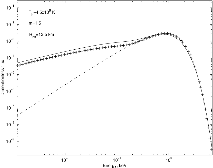
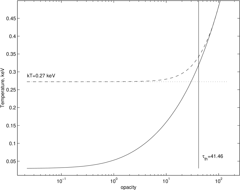
Figure 1: Examples of spectra (left) and temperature profiles (right) obtained for model with $m=1.5$, $R_{ns}=13.5$ km, $Y_{He}=1$. On the left solid line represents the analytical solution, dashed line indicates the diluted blackbody level, ’+’ - results of relaxation method simulation. On the right solid line is the temperature profile obtained from the initial hydrodynamical solution, dashed line is the corrected profile (see text), dotted line is analytically calculated color temperature level.

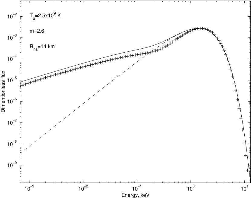
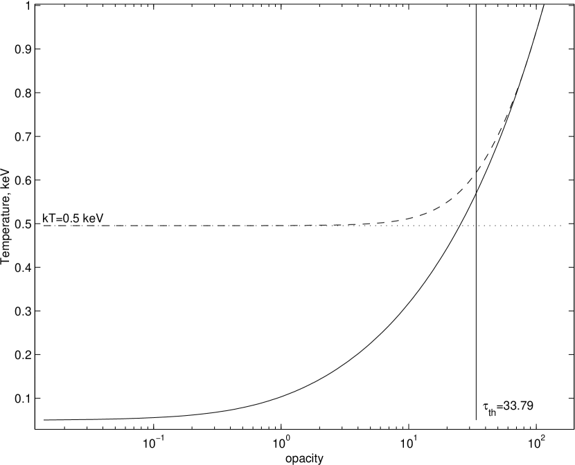
Figure 2: Same as Fig.1 but for the model with $m=2.6$, $R_{ns}=14$ km, $Y_{He}=1$.

To confirm the validity of our analytical approach and to examine the behavior of $p$ and $v_{s}$ in dependence of different input parameters of the problem, we perform numerical modeling of the steady-state radiative transfer process. The whole procedure consisted of three steps.

First, for particular model of neutron star, i. e. for a given mass and radius, we obtain a set of model atmospheres for a chosen set of bottom temperatures. These solutions provide us with runs of thermodynamical and hydrodynamical profiles, sonic point characteristics, masses of the extended envelopes and their loss rates. Second, we solve radiative transfer equation (26) on each model atmosphere obtained with the relaxation method (e.g. Press et al. 1992) on an energy-opacity grid using logarithmic scale on both dimensions. The energy range included 500 grid points. The number of grid points in opacity varied between 100 and 300. The opacity domain included the range $\tau_{s}<\tau<\tau_{max}$, where $\tau_{s}$ is opacity at the sonic point and $\tau_{max}$ was taken large enough to meet safely inequality $\tau_{max}>\tau_{th}$. We used the mixed outer boundary condition (28). Spectrum at the inner bottom of the photosphere was taken a pure black body $B_{\nu}$. Numerical calculations of frequency-dependent radiation field consisted of two runs of our relaxation code. The first run was performed on temperature continuum, obtained from the hydrodynamical solution (see section 2.5). Then we calculated a spectral temperature profile using formulae (31) which exhibits a quite expected behavior. At some region this corrected profile departs from initial temperature profile and levels off at some constant value in absolute agreement with analytic result of section 3.2. It is also in a qualitative agreement with the NTL self-consisted calculation of radiation driven wind structure of X-ray burster. A second run is performed on the corrected profile to get more reliable spectrum shape. At the final third step we compared analytical and numerical solutions. The sonic point provided a natural position to match numerical and analytical solutions. Combining the sonic point parameters, calculated through the solution of equation (25) and using relation (34) we get for the opacity at the sonic point

$$\tau_{s}=\frac{\sigma_{T}}{2m_{p}}r_{s}\rho_{s}\left(1-\frac{Y_{He}}{2}\right).$$ (53)

We calculated and and plotted fluxes given by both methods at the sonic point. A particular value of parameter $p$ for analytic model was obtained by matching value of $kT$ and corrected level of numerically achieved value of photospheric temperature.

We obtained results for approximately 150 different sets of values $T_{b},R_{ns},M_{ns}$ and $Y_{He}$. Examples of numerical calculations of spectra for different neutron star models and fitting them with analytical shapes are presented in Figures 1 and 2. Analytical and numerical shapes match quite well in the wide range of neutron star surface temperatures and both show two distinctive features of outgoing spectrum of expansion stage: diluted black-body like high-frequency component and power law soft excess at the lower part. Dependence of the sonic point opacity presented by (53) describes correctly the dilution process indicating the assumption of atmosphere structure adopted at the analytical model is correct.

Tables 1 and 2, which summarize results for two different neutron star models, are given in order to compare our results with more rigorous calculations (NTL). Taking mass-loss rate as an input parameter, NTL obtained profiles of different quantities throughout the whole atmosphere. They argue that the temperature of burning shell is maintained around $3\times 10^{9}$ K for all models. The temperature of photons departs appreciably from the temperature of ambient matter above photospheric radius and stays practically constant indicating that radiation becomes essentially decoupled from expanded media. We changed the bottom temperature in a wide range of values and inferred the mass-loss rate, the mass of envelope, etc.

Our results are in qualitative agreement with NTL. The crucial physical parameters which define the main spectral signatures are the photospheric radius $r_{ph}$ and its temperature $kT$. Runs of the atmospheric profiles obtained by both approaches are quite similar, although $T_{ph}$ in NTL results is usually $15\%\sim 25\%$ greater than in our models. This difference is explainable. We match isothermal levels given by numerical and analytical calculations and define the obtained value as a photospheric temperature. This is the lowest estimation, because the temperature profile starts to grow before the bottom of the photosphere is reached. NTL define $T_{ph}$ as a matter temperature at $r_{ph}$. A temperature level calculated at the thermalization depth $\tau_{th}$ should compensate the considered difference. The difference in density profiles, which can achieve a factor of two, will affect the spectrum only in the soft part ($\leq 0.2$ keV) where the normalization of the power law component can be changed. This fact does not diminish the validity of our results. The soft component of the spectrum can be represented as an independent fitting shape with a normalization included as an additional fitting parameter. This matter is not crucial at the moment due to the restricted spectral capabilities of current X-ray observing facilities. One can also notice a quick decrease of the envelope mass, and point out a wide variation of $T_{b}$. This discrepancy can be explained by differences in model formulations. Specifically, NTL included helium-burning shells into the model and put the inner boundary condition on the “real” neutron star surface while our model stops where radiation and gas pressures are equal ($y=1$), which is close but still outside of the helium-burning shell. In our approach, part of the bottom of the atmosphere is left out. In fact, the lower the mass-loss rate, the greater the portion of mass missing beyond the point where $y=1$. This is clearly seen from the tables. The temperature at the bottom can be considered as an “effective” instead of the real temperature of helium-burning zone.

As we have already point out that one needs to know the dependencies of $v_{s}$ and $p$ on input parameters to complete the analytical description and thus to employ these results to the fitting of observational X-ray spectra. Analysis of $v_{s}$ and $p$ runs show that $\log v_{s}$ and $\log p$ are linear functions of $\log T_{b}$, $\log R_{ns}$, $\log M_{ns}$ and $\log(2-Y_{He})$. We combine all experiments and fit $v_{s,8}$ and $p$ with a model $cons\times T_{b,9}^{\alpha}r_{b,6}^{\beta}m^{\gamma}(2-Y_{He})^{\eta}$ by the least squares method to get

$$p=7.69\,T_{b,9}^{-0.84}r_{b,6}^{-0.89}m^{0.69}(2-Y_{He})^{-0.22}$$ (54)

$$v_{s,8}=5.46\,T_{b,9}^{-0.71}r_{b,6}^{-0.87}m^{0.63}(2-Y_{He})^{-0.22}$$ (55)

with maximum errors of parameters less than 1%. The ranges of parameters included in fitting are 0.3-7.0 for $T_{b,9}$, 0.6-2.0 for $r_{b,6}$, 0.8-2.7 for $m$ and 0.3-1.0 for $Y_{He}$. These results can be used to substitute $p$ and $v_{s,8}$ in equations (50)-(52). Now we have consistent system of equations, which should yield X-ray spectrum of burster in the form of function of only input physical parameters, i. e. neutron star mass, radius, surface temperature and elemental abundance.

5 Final form of the profile for spectral fitting

The fact that spectra obtained are a black-body like almost everywhere except for small values of energies allows us to proceed with simplification of the formula (39). First we note that due to (47) and smallness of $x$

$$t_{th}=\frac{4}{7}\sqrt{3\Psi(x)D}\,\tau_{th}^{7/4}=2\frac{\sqrt{2\Psi(x)}}{p}\simeq 2\frac{\sqrt{\ln(2.35/x)}}{px},$$ (56)

for the soft part of spectrum. Here $x=h\nu/kT$, $\Psi(x)$ and $D$ are defined in formulae (27) and (46) correspondingly. Because $t_{th}$ is large for small values $x$ we can use approximation of the modified Bessel function of the second kind for large arguments

$$K_{p}(x)\approx\sqrt{\frac{\pi}{2x}}\,e^{-x},$$

and rewrite equation (39) as follows

$$J(\tau,x)=B_{\nu}\left(\frac{\tau}{\tau_{th}}\right)^{2}\left[\frac{\Gamma(3/7)}{\Gamma(11/7)}z^{8/7}+\frac{4}{7\Gamma(11/7)}z^{1/14}e^{-2z}\right]=$$

$$=B_{\nu}\left(\frac{\tau}{\tau_{th}}\right)^{2}\left[2.32\,z^{8/7}+0.64\,z^{1/14}e^{-2z}\right],$$ (57)

where

$$z=\frac{\sqrt{\ln(2.35/x)}}{px}.$$

Here we rewrite the dilution factor in terms of opacity using relation (40). Clearly, the second term in the parenthesis of formula (57) is significant only where $z$ becomes small ($x$ becomes large) and the spectrum shape “adjusts” to the black-body component. In turn, the first term of equation (57) represents the power law component of the lower part of spectrum with the slope 6/7, which can be shown by simple similarity (see also T94)

$$B_{\nu}z^{8/7}\sim\frac{x^{2}}{x^{8/7}}=x^{6/7}.$$

Another important advantage of this term is that it vanishes for large values of $x$. This fact gives us opportunity to construct convenient and accurate formula for observational spectra fitting. We drop the second term in equation (57) and adjust to the diluted black-body shape by means of quadratic power combination as follows

$$J(\tau,x)=B_{\nu}\left(\frac{\tau}{\tau_{th}}\right)^{2}\left[1+5.34\,z^{16/7}\right]^{1/2}.$$ (58)

Comparison of shapes given by formula (58) with exact solution (39) shows that they deviate from each other by less than 2% which is more than acceptable in contemporary astrophysical observational data analysis. Using the explicit form of $z$ and the form of outgoing flux equation (58) can be rewritten in the form

$$F_{\nu}=\frac{4\pi}{3}\frac{dJ_{\nu}}{d\tau}=\frac{8\pi}{3}B_{\nu}\frac{\tau_{s}}{\tau_{th}^{2}}\left\{1+5.34\left[\frac{\ln(2.35/x)}{p^{2}x^{2}}\right]^{8/7}\right\}^{1/2}.$$ (59)

Equation (53) yields useful relationship for the dilution coefficient in the manner similar to (50)-(52)

$$\frac{8\pi}{3}\frac{\tau_{s}}{\tau_{th}^{2}}=\frac{5.07\times 10^{-5}r_{b,6}^{10/7}T_{b,9}^{10/17}p^{16/7}}{m^{11/7}v_{s,8}^{2/7}(2-Y_{He})^{1/7}}.$$ (60)

Substituting results of parameter fitting (54)-(55), we get

$$\frac{8\pi}{3}\frac{\tau_{s}}{\tau_{th}^{2}}=3.31\times 10^{-3}r_{b,6}^{-0.36}\,T_{b,9}^{-0.29}m^{-0.17}(2-Y_{He})^{-0.58},$$ (61)

$$p=7.69\,T_{b,9}^{-0.84}r_{b,6}^{-0.89}m^{0.69}(2-Y_{He})^{-0.22}.$$ (54)

Here, again, $r_{b,6}$, $T_{b,9}$ and $m$ are the neutron star radius, surface temperature and mass in units of $10^{6}$ cm, $10^{9}$ Kelvin and solar mass respectively. Now we have provided our spectrum profile (59) with expressions for parameter $p$ (54) and the dilution factor (61). These three formulae constitute the final analytical results of this paper.

6 Discussion

The model and derivations presented above assume that plasma consists of fully ionized hydrogen and helium. In reality, this assumption can be too simplistic. For instance, in the case of the recently discovered super-burst (Strohmayer & Brown, 2001), a sufficient fraction of material should be represented by heavier elements. These long and powerful bursts are also considered to be due to the nuclear runaway burning in the carbon “ocean” under the neutron star surface. In this section we discuss how our model can be adjusted for study of this phenomenon. The approach as a whole does not change, but some formulae have to be modified in order to account for the different plasma composition.

First, we note that for plasma which consists of a single ionized element, we have for the mean molecular weight

$$\mu=\frac{A}{1+Z},$$

and for the electron number density

$$n_{e}=\frac{\rho}{Am_{p}}Z,$$

where $A$ and $Z$ are the atomic weight and the atomic number of the corresponding element. In the general case of heterogenous elements, each represented by weight abundance $Y_{i}$, we write

$$\mu=\frac{1}{\sum Y_{i}(1+Z_{i})/A_{i}}.$$ (62)

$$n_{e}=\frac{\rho}{m_{p}}\sum\frac{Z_{i}}{A_{i}}Y_{i}.$$ (63)

In the hydrodynamic part of this study, these modifications will affect only the form of the terms and factors containing $Y_{He}$. In the radiation transfer section, the form of $\alpha_{ff}/\alpha_{T}$ will require more careful treatment. According to Rybicki & Lightman (1979), the free-free absorption coefficient is

$$\alpha_{ff}=3.7\times 10^{8}\,T^{-1/2}\overline{Z^{2}n_{i}}n_{e}\,\nu^{-3}(1-e^{-h\nu/kT})\,\tilde{g}_{ff},$$ (64)

where

$$\overline{Z^{2}n_{i}}=\sum Z_{i}^{2}n_{i}=\frac{\rho}{m_{p}}\sum\frac{Z_{i}^{2}}{A}Y_{i}.$$ (65)

In the case of a hydrogen-helium plasma this factor is conveniently represented just by gas density, i. e.

$$\overline{Z^{2}n_{i}}=n_{H}+4n_{He}=\frac{\rho}{m_{p}}(Y_{H}+Y_{He})=\frac{\rho}{m_{p}},$$

which yields the equation (27). In general, one should use expressions (64) and (65) to find the correct form of $\alpha_{ff}/\alpha_{T}$ relevant to the specific chemical composition.

To be more instructive we conduct such a modification for the case when the plasma has a substantial carbon fraction. Using (62), (63) and (65), we write for hydrogen-helium-carbon gas

$$\mu=\frac{12}{24Y_{H}+9Y_{He}+7Y_{C}}=\frac{4}{8-5Y_{He}-17Y_{C}/3},$$ (66)

$$n_{e}=\frac{\rho}{m_{p}}\left(1-\frac{Y_{He}+Y_{C}}{2}\right),$$ (67)

and

$$\overline{Z^{2}n_{i}}=\frac{\rho}{m_{p}}(Y_{H}+Y_{He}+3Y_{C})=\frac{\rho}{m_{p}}(1+2Y_{C}).$$ (68)

Correspondingly, in all formulae the factor $(2-Y_{He})$ will be replaced by $(2-Y_{He}-Y_{C})$ and $(8-5Y_{He})$ by $(8-5Y_{He}-17Y_{C}/3)$. Additionally, the right-hand side of equation (27) has to be multiplied by the factor of $(1+2Y_{C})$. Clearly, this modification will add the fifth free parameter $Y_{C}$ to the model. Using the general methodology outlined in this paper one should be able to produce solutions for the parameter $p$ and the dilution factor. The problem which can arise from the inclusion of heavy elements is the possibility for heavy ions to be only partly ionized. The ionization degree can also vary throughout the atmosphere. Because full ionization and constancy of the gas’s chemical composition are the basic assumptions of the adopted approach, we cannot explicitly include the effect of ionization in our model. Instead, it can be accounted for in a manner similar to our temperature profile correction. First, the approximate atmospheric profiles can be obtained by assuming full ionization. Then, the ionization degree can be calculated by solving the Saha equation, and using this solution as a zero-order approximation of the atmospheric temperature and the electron number density profiles. Finally, one should proceed by solving the hydrodynamic problem, in which the partial ionization of heavy elements is taken into account.

For reasons mentioned above, it is also a problem to include the proper physics for the transport of heavy nuclei to the outer layers. Two major processes can contribute to this element flow. Bulk motion mixing should dominate in the convection zone close to the bottom of the atmosphere. In the outer layers, a strong radiative push should govern the process, because of the large resonance cross-sections of the heavy elements. The general problem of heavy ions mixing is quite difficult and requires a rigorous approach, which is out of scope of this paper.

As far as the boundary conditions are concerned, modeling of carbon nuclear flashes will require higher bottom temperatures. Temperature of the carbon burning zone is argued to be about $10^{10}$ K [see Strohmayer & Brown (2001)], which is close to the upper boundary for the bottom temperature $T_{b}$ used in our calculations. No peculiarities of the approach were detected in the case of very high bottom temperatures. Extremely high temperatures will require the correct form of the opacity coefficient $\kappa$ (Paczynski, 1983), instead of equation (2), which represents a simplified formula for $\kappa$ in the case of modest temperatures.

Another important issue is the correct accounting for the line emission of heavy elements which is detected in the spectral analysis of super-bursts. Strohmayer & Brown (2001) argued that this phenomena is due to reflection from the accretion disk during the burst. One can estimate the disk heating time by using the standard Shakura-Sunyaev accretion disk model (Shakura & Sunyaev, 1973) and the fact that approximately 10% of the burst luminosity is absorbed by the inner part of the disk (Lapidus & Sunyaev, 1985). Simple estimates give a timescale of less than a second assuming a mass-accretion rate of the order of Eddington or less for the disk accretion regime, and a burst luminosity greater than 5% of Eddington, which is detected during several thousand seconds of observation of the super-burst in 4U 1820-30 Consequently, the observed spectral feature of the K$\alpha$ line should rather be generated in the burst atmosphere than in the disk. The disk gains the temperature of the X-ray radiation very quickly.

Unfortunately, the origin and behavior of the spectral line features still remain unexplained. The authors plan to inlcude the spectral line effect in the relaxation method, in order to calculate the line emission during the X-ray burst and to compare this with the observed spectra.

Relativistic effects are usually negligible during the strong X-ray burst due to the significant radial expansion and the fact that the outgoing spectrum formation occurs at the outer layers of the atmosphere. General relativistic effects become important at the contraction stage when the extended envelope recedes close to the NS surface [see Lewin, Paradijs & Taam (1993)]. Haberl & Titarchuk (1995) applied the full general relativity approach for a derivation of NS mass-radius relation in 4U 1820-30 using EXOSAT observations and the T94 model.

7 Conclusion

This paper follows a common idea of the last decade to fit observational and numerical spectra with some model, mostly black-body shapes, to obtain spectral softening/hardening factors (London et al., 1986). We improve this technique in several ways. We use for fitting more realistic non-blackbody spectral profile, which accounts for the observed power law soft excess of X-ray burster spectra. The temperature profile is corrected by solving the temperature equation. The existence of the isothermal photosphere during X-ray bursts is confirmed numerically and analytically. Finally, we analytically obtain the multiplicative (dilution) factor which is not a parameter of fitting anymore but self-consistently incorporated in the model.

We show how the theoretical study of radiatively driven wind phenomenon can produce useful techniques for analyzing observational data. It can fulfill the needs of new emerging branches of observational X-ray astronomy such as a very promising discovery of super-bursts (Strohmayer & Brown, 2001), which exhibit photospheric expansion and spectral modifications relevant to extended atmospheres. We present the analytical theory of strong X-ray bursts, which include effects of Comptonization and free-free absorption. Partly presented in some earlier publications, this area of the study of the X-ray burst spectral formation was lacking a detailed and self-consistent account. We use numerical simulation to validate our analytical theory and to link our solution to energy axes. We show how this information can be extracted from spectral data. We provide the analytical expression for the X-ray burst spectral shape, which depends only upon input physical parameters of the problem: neutron star mass, radius, surface temperature and elemental abundance. Expressions for color ratios and dilution coefficient are also given.

Authors thank Peter Becker for valuable comments and suggestions which improved the paper. We are greatful to Menas Kafatos for encouragement and to Center for Earth Science and Space Research (GMU) for the support of this research. We appreciate the thorough analysis of the presented work by the referee.

Appendix A Analytic solution for the radiative transfer problem

We look for the solution of equation (35) in the form

$$J(\tau,x)=\left(\frac{\tau}{\tau_{th}}\right)^{2}B_{\nu}(\tau_{th})+\tilde{J}(\tau,x).$$ (A1)

The basic idea is to separate the high-frequency (diluted black body) and the low-frequency $\tilde{J}(\tau,x)$ parts of spectrum, where different physical processes dominate. Kompaneets operator $L_{\nu}$ acting upon black body shape vanishes and we neglect $L_{\nu}(\tilde{J})$, which allows us to get the solution of radiative transfer problem analytically. At this point $\tau_{th}$ is a parameter of the problem. The algorithm of determination of $\tau_{th}$ will be described separately. Substituting (A1) into (35) we found for $\tilde{J}(\tau,x)$

$$\frac{\partial}{\partial\tau}\left(\frac{1}{\tau}\frac{\partial\tilde{J}}{\partial\tau}\right)-\frac{3}{\tau}\frac{\alpha_{ff}}{\alpha_{T}}\tilde{J}=-\frac{3}{\tau}\frac{\alpha_{ff}}{\alpha_{T}}B_{\nu}\left[1-\left(\frac{\tau}{\tau_{th}}\right)^{2}\right],$$ (A2)

with a boundary condition

$$\tilde{J}_{\nu}|_{\tau=\tau_{th}}=0.$$ (A3)

The solution satisfying this condition is presented by

$$\tilde{J}(\tau,x)=\frac{1}{pW}y_{1}(\tau)\int_{0}^{\tau_{th}}y_{2}(\tau)f(\tau)\,d\tau,$$ (A4)

where $p(\tau)=\frac{1}{\tau}$ and $W(\tau)$ is the Wronskian

$$W=\left|\begin{array}[]{cc}y_{1}&y_{2}\\ y_{1}^{\prime}&y_{2}^{\prime}\end{array}\right|=-\frac{7}{4}\tau.$$ (A5)

Thus the product

$$pW=-\frac{7}{4}.$$

Functions $y_{1}(x)$ and $y_{2}(x)$ are

$$y_{1}(\tau)=\tau I_{4/7}\left(\frac{4}{7}\sqrt{3D\Psi(x)}\,\tau^{7/4}\right),$$ (A6)

$$y_{2}(\tau)=\tau K_{4/7}\left(\frac{4}{7}\sqrt{3D\Psi(x)}\,\tau^{7/4}\right),$$ (A7)

where $I_{\nu}(x)$ and $K_{\nu}(x)$ are modified Bessel function of the first and the second types respectively.

The function $f(\tau)$ in (A4) is the right hand side of equation (A2), namely

$$f(\tau)=-\frac{3}{\tau}\frac{\alpha_{ff}}{\alpha_{T}}=-3\,\tau^{1/2}D\Psi(x)B_{\nu}\left[1-\left(\frac{\tau}{\tau_{th}}\right)^{2}\right].$$ (A8)

We introduce a new variable $t$

$$t=\frac{4}{7}\sqrt{3D\Psi(x)}\,\tau^{7/4},$$ (A9)

and rewrite solution (A4) as

$$\tilde{J}(t,x)=B_{\nu}t^{4/7}I_{4/7}(t)\int_{0}^{t_{th}}t^{3/7}K_{4/7}(t)\left[1-\left(\frac{t}{t_{th}}\right)^{8/7}\right]dt.$$ (A10)

Using the properties of modified Bessel functions

$$\int x^{p}K_{p-1}dx=-x^{p}K_{p}+C\quad\mathrm{and}\quad K_{p}=K_{-p}$$

we evaluate the integrals in (A10)

$$\int_{0}^{t_{th}}t^{3/7}K_{4/7}(t)\,dt=-t^{3/7}K_{3/7}(t)\Bigl{|}_{0}^{t_{th}}=\frac{\Gamma\left(\frac{3}{7}\right)}{2^{4/7}}-t_{th}^{3/7}K_{3/7}(t_{th}),$$

$$\int_{0}^{t_{th}}t^{11/7}K_{4/7}(t)\,dt=-t^{11/7}K_{11/7}(t)\Bigl{|}_{0}^{t_{th}}=\Gamma\left(\frac{11}{7}\right)2^{4/7}-t_{th}^{11/7}K_{11/7}(t_{th}).$$

Finally $\tilde{J}(t,x)$ takes the form

$$\tilde{J}(t,x)=B_{\nu}t^{4/7}I_{4/7}(t)\left[\frac{\Gamma\left(\frac{3}{7}\right)}{2^{4/7}}-\frac{\Gamma\left(\frac{11}{7}\right)2^{4/7}}{t_{th}^{8/7}}+t_{th}^{3/7}(K_{11/7}(t_{th})-K_{3/7}(t_{th}))\right]=$$

$$\tilde{J}(t,x)=B_{\nu}t^{4/7}I_{4/7}(t)\left[\frac{\Gamma\left(\frac{3}{7}\right)}{2^{4/7}}-\frac{\Gamma\left(\frac{11}{7}\right)2^{4/7}}{t_{th}^{8/7}}+\frac{8}{7}\,t_{th}^{-4/7}K_{4/7}(t_{th})\right].$$ (A11)

The last formula is a solution of equation (35). We can simplify this form by noting that we are interested in the solution in the outer layers of atmosphere (emergent spectrum) where $\tau\rightarrow 0$ and $t\rightarrow 0$, and we can use the asymptotic form for small arguments

$$I_{p}(x)\approx\frac{1}{\Gamma(p+1)}\left(\frac{x}{2}\right)^{p}.$$

Making this substitution and putting the result into expression for $J(\tau,x)$ we find that second term in $\tilde{J}(\tau,x)$ cancels with diluted blackbody term in $J(\tau,x)$, which takes the form

$$J(t,x)=B_{\nu}\frac{t^{8/7}}{2^{4/7}\Gamma\left(\frac{11}{7}\right)}\left[\frac{\Gamma\left(\frac{3}{7}\right)}{2^{4/7}}+\frac{8}{7}\,t_{th}^{-4/7}K_{4/7}(t_{th})\right].$$ (A12)

Appendix B Solution of the temperature equation

Substituting relation (41) into the equation of radiative diffusion, multiplying it by $x^{2}$ and integrating over the energy range from $x_{*}$ to $\infty$ we get

$$\frac{1}{3}\left(\frac{d^{2}R}{d\tau^{2}}-\frac{1}{\tau}\frac{dR}{d\tau}\right)\int_{x_{*}}^{\infty}\frac{x^{2}}{e^{x}-1}\,dx=[R(\tau)-1]\int_{x_{*}}^{\infty}\frac{x^{2}}{e^{x}-1}\frac{\alpha_{ff}}{\alpha_{T}}\,dx,$$ (B1)

where integrals can be approximated as

$$\int_{x_{*}}^{\infty}\frac{x^{2}}{e^{x}-1}\approx\int_{0}^{\infty}x^{2}e^{-x}dx=2$$

and, noting that $\alpha_{ff}/\alpha_{T}=D\Psi(x)\,\tau^{3/2}\approx D\,\tau^{3/2}\tilde{g}(x)/x^{2}$ we obtain

$$\int_{x_{*}}^{\infty}\frac{x^{2}}{e^{x}-1}\frac{\alpha_{ff}}{\alpha_{T}}\,dx\approx D\,\tau^{3/2}\int_{x_{*}}^{\infty}\frac{\tilde{g}(x)}{x}\,dx\approx\frac{1}{4}\ln^{2}\frac{2.25}{x_{*}}D\,\tau^{3/2}.$$

Here we used the fact that $\tilde{g}(x)\approx\frac{1}{2}\ln(2.35/x)$. The equation for $R(\tau)$ gets the form

$$\frac{d^{2}R}{d\tau^{2}}-\frac{1}{\tau}\frac{dR}{d\tau}=\frac{3}{8}\ln^{2}\frac{2.25}{x_{*}}D\tau^{3/2}[R(\tau)-1]=\tilde{D}\tau^{3/2}[R(\tau)-1].$$ (B2)

Boundary conditions for this equation are

$$\begin{array}[]{cc}\tau\rightarrow 0&R(\tau)\rightarrow 0,\\ \tau\rightarrow\infty&R(\tau)\rightarrow 1.\end{array}$$ (B3)

A general solution of equation (29) is

$$R(\tau)=1+\tau Z_{4/7}\left(\frac{4}{7}i\sqrt{\tilde{D}}\tau^{7/4}\right),$$ (B4)

where $Z_{4/7}(z)=c_{1}K_{4/7}(z)+c_{2}I_{4/7}(z)$. In derivation of this formula we take into account a well known theorem from ODE theory that general solution of inhomogeneous ODE is the sum of a general solution of the corresponding homogeneous ODE and some particular solution of the inhomogeneous ODE, which is chosen equals to unity in our case. The second boundary condition and the fact that

$$\begin{array}[]{cc}K_{4/7}(z)\rightarrow 0&z\rightarrow\infty,\\ I_{4/7}(z)\rightarrow\infty&z\rightarrow\infty\end{array}$$

leave only $c_{1}$ nonzero, and the first boundary condition gives us the value for $c_{1}$, namely

$$c_{1}=-\frac{1}{{}_{\tau}\varinjlim_{0}\tau K_{4/7}\left(\frac{4}{7}\sqrt{\tilde{D}}\,\tau^{7/4}\right)}=-\frac{2^{3/7}}{\Gamma\left(\frac{4}{7}\right)\tau_{th}},$$

where we put $\tau_{th}=\left(\frac{4}{7}\sqrt{\tilde{D}}\right)^{-4/7}$. Then $R(\tau)$ reduces to

$$R(\tau)=1-\frac{2^{3/7}}{\Gamma\left(\frac{4}{7}\right)}\frac{\tau}{\tau_{th}}K_{4/7}\left[\left(\frac{\tau}{\tau_{th}}\right)^{7/4}\right].$$ (B5)

Taylor series expansion of $K_{4/7}$ over $\tau/\tau_{th}$ yields for $R(\tau)$ useful relation

$$R(\tau)=\frac{\Gamma\left(\frac{3}{7}\right)}{2^{8/7}\Gamma\left(\frac{11}{7}\right)}\left(\frac{\tau}{\tau_{th}}\right)^{2}.$$ (B6)

Appendix C Condition at the sonic point (derivation of $Y_{s}$)

We can rewrite the partial derivative in (18) using the obvious relation

$$\left(\frac{\partial P}{\partial\rho}\right)_{\Xi}=\frac{\partial P}{\partial T}\left(\frac{\partial T}{\partial\rho}\right)_{\Xi}+\frac{\partial P}{\partial y}\left(\frac{\partial y}{\partial\rho}\right)_{\Xi}.$$

Differentiating the equation of state (8) we obtain derivatives of pressure

$$\frac{\partial P}{\partial T}=\left(1+\frac{1}{y}\right)\frac{4aT^{3}}{3}\quad\mathrm{and}\quad\frac{\partial P}{\partial y}=-\frac{1}{y^{2}}\frac{aT^{4}}{3},$$

and differentiating (21) with respect to $\rho$ we get

$$\left(\frac{\partial T}{\partial\rho}\right)_{\Xi}=-\frac{T}{\lambda}\left(\frac{1}{y}+4\right)\left(\frac{\partial y}{\partial\rho}\right)_{\Xi}.$$

From the other hand differentiation of (9) gives us

$$\frac{a\mu m_{p}}{3k}\left(\frac{3T^{2}}{y}\frac{\partial T}{\partial\rho}-\frac{T^{3}}{y^{2}}\frac{\partial y}{\partial\rho}\right)=1.$$

Combination with the previous equation it yields:

$$\left(\frac{\partial y}{\partial\rho}\right)_{\Xi}=-\frac{3k}{a\mu m_{p}}\frac{y^{2}}{T^{3}}\left(\frac{\lambda}{\lambda+3(1+4y)}\right),$$

$$\left(\frac{\partial T}{\partial\rho}\right)_{\Xi}=\frac{3k}{a\mu m_{p}T^{2}}\left(\frac{y(1+4y)}{\lambda+3(1+4y)}\right).$$

Now, combining all found derivatives we have

$$\left(\frac{\partial P}{\partial\rho}\right)_{\Xi}=\frac{k}{\mu m_{p}}\left[4\left(1+\frac{1}{y}\right)\left(\frac{y(1+4y)}{\lambda+3(1+4y)}\right)+\frac{\lambda}{\lambda+3(1+4y)}\right]T$$

or in a more compact form

$$\left(\frac{\partial P}{\partial\rho}\right)_{\Xi}=\frac{k}{\mu m_{p}}\left[\frac{\lambda+4(1+y)(1+4y)}{\lambda+3(1+4y)}\right]T,$$ (C1)

which is, in fact, a sonic point condition (18).

Appendix D Reduction of Hydrodynamical Problem to First-Order ODE

We derive an expression for the derivative of velocity $v_{y}$ through $v$ and $y$.

We substitute the temperature profile found in (21) to (5) to obtain $\rho$ as a function of $y$

$$\rho=\rho(y)=\frac{a\mu m_{p}T_{b}^{3}}{3k}\,y^{-3/\lambda-1}\exp\left[-\frac{12(y-1)}{\lambda}\right].$$

Using this expression for $\rho(y)$ and equation (12) we get

$$r=r(v,y)=\left(\frac{\Phi}{4\pi}\right)^{1/2}\rho^{-\frac{1}{2}}v^{-\frac{1}{2}}=\left(\frac{3\Phi k}{4\pi a\mu m_{p}T_{b}^{3}}\right)^{1/2}y^{\frac{3}{2\lambda}+\frac{1}{2}}\exp\left[\frac{6(y-1)}{\lambda}\right]v^{-\frac{1}{2}}.$$

Then we get derivatives

$$\frac{dr}{dy}=r\left[\left(\frac{3}{2\lambda}+\frac{1}{2}\right)\frac{1}{y}+\frac{6}{\lambda}\right],$$

$$\frac{dr}{dv}=-\frac{r}{2v}.$$

Differentiation of (21) also gives us

$$\frac{dT}{dy}=T_{b}\,y^{-1/\lambda}\exp\left[-\frac{4(y-1)}{\lambda}\right]\left(-\frac{1}{\lambda y}-\frac{4}{\lambda}\right)=-\frac{T}{\lambda}\left(4+\frac{1}{y}\right).$$

By a combination of all these derivatives we obtain

$$\frac{dT}{dr}=\frac{dT}{dy}\frac{dy}{dr}=\frac{dT}{dy}\left(\frac{\partial r}{\partial y}+\frac{\partial r}{\partial v}\frac{dv}{dy}\right)^{-1}=-\frac{2T(4y+1)}{r\lambda y}\left[\left(\frac{3}{\lambda}+1\right)\frac{1}{y}+\frac{12}{\lambda}-\frac{v^{\prime}}{v}\right]^{-1}.$$

Substitution of it into (5) yields

$$L_{r}=-\frac{16\pi ckr^{2}y}{\mu m_{p}\kappa}\frac{dT}{dr}=\frac{32\pi ck}{\mu m_{p}\lambda\kappa_{0}(2-Y_{He})}\frac{(4y+1)(1+\alpha T)Tr}{\left[\left(3/\lambda+1\right)1/y+12/\lambda-v^{\prime}/v\right]}.$$

But from (13) we also have

$$L_{r}=\Psi-\Phi\left(h+\frac{v^{2}}{2}-\frac{GM_{ns}}{r}\right).$$

Equating the last two expressions for $L_{r}$ we finally find $v_{y}$ as

$$v_{y}^{\prime}=f(v,y)=v\left[\left(1+3\frac{1+4y}{\lambda}\right)\frac{1}{y}-75.2\frac{rT(8-5Y_{He})(1+4y)(1+\alpha T)}{\lambda r_{b,6}T_{b,9}(\Psi/\Phi-v^{2}/2-h+GM_{ns}/r)}\right].$$

Here $r_{b,6}$ and $T_{b,9}$ represent neutron star radius and the bottom temperature of atmosphere in terms of $10^{6}$ cm and $10^{9}$ K correspondingly.

Table 1: Parameters for model $m=1.5$, $R_{ns}=13.5$ km, $Y_{He}=1$

$T_{b}$	$kT$	$T/T_{0}$	$\tau_{th}$	$p$		$\Phi$	$M_{env}$		$T_{s}$	$v_{s}$	$r_{s}$	$r_{ph}$
$10^{9}$K	keV						$10^{22}$g		$0.1$ keV	$10^{3}$ km/s	$10^{3}$km	$10^{3}$km
7.0	0.197	0.099	45.1	1.	56	93.9	173.	3	0.21	1.31	57.9	4.16
6.5	0.208	0.105	44.7	1.	64	87.2	128.	9	0.22	1.39	51.6	3.71
6.0	0.221	0.111	44.1	1.	75	80.5	93.	6	0.24	1.48	45.6	3.28
5.5	0.236	0.118	43.3	1.	87	73.8	66.	1	0.25	1.58	39.9	2.88
5.0	0.252	0.127	42.4	2.	02	67.1	45.	1	0.27	1.70	34.5	2.50
4.5	0.272	0.137	41.5	2.	20	60.4	29.	6	0.29	1.84	29.4	2.14
4.0	0.295	0.148	40.3	2.	42	53.7	18.	5	0.32	2.01	24.6	1.80
3.5	0.324	0.163	39.0	2.	71	46.9	10.	9	0.35	2.22	20.1	1.48
3.0	0.359	0.180	37.4	3.	09	40.2	5.	86	0.39	2.50	16.0	1.19
2.5	0.406	0.204	35.6	3.	60	33.5	2.	83	0.44	2.85	12.2	0.92
2.0	0.470	0.236	33.4	4.	34	26.8	1.	16	0.51	3.36	8.83	0.67
1.75	0.510	0.257	32.2	4.	85	23.5	0.	68	0.55	3.69	7.29	0.56
1.5	0.565	0.284	30.8	5.	53	20.1	0.	37	0.61	4.12	5.86	0.45
1.25	0.634	0.318	29.2	6.	44	16.8	0.	179	0.68	4.69	4.53	0.36
1.1	0.686	0.344	28.0	7.	18	14.8	0.	108	0.74	5.12	3.80	0.30
1.0	0.727	0.365	27.2	7.	78	13.4	0.	074	0.78	5.47	3.33	0.27
0.9	0.775	0.389	26.3	8.	51	12.1	0.	049	0.84	5.87	2.89	0.23
0.8	0.831	0.417	25.3	9.	40	10.7	0.	031	0.90	6.36	2.46	0.20
0.7	0.898	0.451	24.3	10.	5	9.4	0.	018	0.97	6.95	2.06	0.17
0.6	0.981	0.492	23.0	12.	0	8.0	0.	010	1.06	7.69	1.68	0.14
0.5	1.086	0.545	21.6	14.	0	6.7	0.	005	1.17	8.65	1.33	0.11
0.4	1.224	0.614	19.9	17.	0	5.4	0.	002	1.32	9.95	1.01	0.09
0.3	1.417	0.711	17.8	21.	9	4.0	0.	001	1.53	11.8	0.71	0.07

Table 2: Parameters for model $m=2.6$, $R_{ns}=14.0$ km, $Y_{He}=1$.

$T_{b}$	$kT$	$T/T_{0}$	$\tau_{th}$	$p$		$\Phi$		$M_{env}$		$T_{s}$	$v_{s}$		$r_{s}$		$r_{ph}$
$10^{9}$K	keV							$10^{22}$g		$0.1$ keV	$10^{3}$ km/s		$10^{3}$km		$10^{3}$km
7.0	0.248	0.110	45.1	2.	12	56.	2	115.	8	0.242	1.	80	53.	4	3.53
6.5	0.261	0.116	44.5	2.	24	52.	2	86.	1	0.256	1.	90	47.	7	3.15
6.0	0.277	0.123	43.6	2.	40	48.	2	62.	6	0.271	2.	02	42.	2	2.80
5.5	0.294	0.131	42.6	2.	58	44.	1	44.	2	0.288	2.	16	36.	9	2.46
5.0	0.313	0.139	41.5	2.	80	40.	1	30.	2	0.308	2.	32	31.	9	2.15
4.5	0.337	0.150	40.3	3.	07	36.	1	19.	8	0.331	2.	52	27.	2	1.84
4.0	0.364	0.162	39.0	3.	40	32.	1	12.	4	0.359	2.	75	22.	8	1.56
3.5	0.398	0.177	37.4	3.	82	28.	1	7.	27	0.394	3.	04	18.	7	1.29
3.0	0.440	0.196	35.7	4.	36	24.	1	3.	93	0.437	3.	41	14.	9	1.04
2.5	0.495	0.220	33.8	5.	12	20.	1	1.	90	0.494	3.	89	11.	4	0.81
2.0	0.570	0.254	31.5	6.	21	16.	1	0.	78	0.572	4.	58	8.	24	0.59
1.75	0.620	0.276	30.2	6.	97	14.	0	0.	46	0.623	5.	03	6.	80	0.50
1.5	0.682	0.304	28.7	7.	97	12.	0	0.	25	0.687	5.	61	5.	47	0.40
1.25	0.763	0.339	27.0	9.	33	10.	0	0.	121	0.770	6.	38	4.	24	0.32
1.1	0.824	0.366	25.9	10.	4	8.	83	0.	073	0.833	6.	96	3.	56	0.27
1.0	0.872	0.388	25.1	11.	3	8.	03	0.	050	0.883	7.	43	3.	12	0.24
0.9	0.928	0.413	24.2	12.	4	7.	22	0.	033	0.940	7.	98	2.	71	0.21
0.8	0.993	0.442	23.3	13.	7	6.	42	0.	021	1.008	8.	63	2.	31	0.18
0.7	1.072	0.477	22.2	15.	4	5.	62	0.	012	1.089	9.	43	1.	94	0.15
0.6	1.169	0.520	21.0	17.	6	4.	82	0.	007	1.188	10.	4	1.	59	0.13
0.5	1.292	0.575	19.7	20.	6	4.	01	0.	003	1.313	11.	7	1.	26	0.10
0.4	1.455	0.647	18.1	24.	9	3.	21	0.	001	1.479	13.	5	0.	95	0.08
0.3	1.682	0.749	16.2	32.	0	2.	41	0.	0005	1.710	16.	0	0.	67	0.06

References

- Ebisuzaki (1987) Ebisuzaki, T., 1987, PASJ, 39, 287
- Ebisuzaki al. (1983) Ebisuzaki, T., Hanawa, T., & Sugimoto, D. 1983, PASJ, 35, 17 (EHS)
- Greene (1959) Greene, J., 1959, ApJ, 130, 693
- Grindlay et al. (1975) Grindlay, J. E., & Heise, J. 1975, IAU Circ., No.2879
- Haberl & Titarchuk (1995) Haberl, F., & Titarchuk, L.G. 1995, A&A, 299, 414
- Kuulkers et al. (2001) Kuulkers, E., Homan, J., van der Klis M., Levin, W.H.G., Mendez, M. 2001 , accepted to A&A
- Lapidus (1991) Lapidus, I., I. 1991, ApJ, 377, L93
- Lapidus & Sunyaev (1985) Lapidus, I., I., Sunyaev, R., A., 1985, MNRAS, 217, 291
- Lewin, Paradijs & Taam (1993) Lewin, W. H. G.,van Paradijs, J., & Taam, R. E. 1993, Space Sci. Rev., 62, 223
- London et al. (1986) London, R., A., Taam, R., E., Howard, H., W. 1986, ApJ, 306, 170
- Nobili,Turolla & Zamperi. (1991) Nobili, L., Turolla, R., & Zamperi, L. 1991, ApJ, 383, 250
- Nobili et al. (1994) Nobili, L., Turolla, R., & Lapidus, I. I. 1994, ApJ, 433, 276 (NTL)
- Paczynski (1983) Paczynski, B., 1983, ApJ, 267, 315
-
Press et al. (1992)
Press, W. H., Teulkolsky, S.A., Vettering, W.T.,
& Flannery B.P. 1992 Numerical Recipes
(Cambridge: University Press) -
Rybicki & Lightman (1979)
Rybicki, G. B., & Lightman A.P. 1979 Radiative Processes
in Astrophysics
(New York: Wiley) - Thorne (1981) Thorne, K. S. 1981, MNRAS, 194, 439
- Titarchuk (1994) Titarchukk, L. G. 1994, ApJ, 429, 340 (T94)
- Strohmayer & Brown (2001) Strohmayer E. T., Brown F. E., (2001), in press (astro-ph/0108420).
- Shakura & Sunyaev (1973) Shakura, N., I., Sunyaev, R., A., 1973, A&A, 24, 337