A Fast, Accurate and Robust Algorithm For Transferring Radiation in Three-Dimensional Space

Abstract

We have developed an algorithm for transferring radiation in three-dimensional space. The algorithm computes radiation source and sink terms using the Fast Fourier Transform (FFT) method, based on a formulation in which the integral of any quantity (such as emissivity or opacity) over any volume may be written in the classic convolution form. The algorithm is fast with the computational time scaling as $N(\log N)^{2}$, where $N$ is the number of grid points of a simulation box, independent of the number of radiation sources. Furthermore, in this formulation one can naturally account for both local radiation sources and diffuse background as well as any extra external sources, all in a self-consistent fashion. Finally, the algorithm is completely stable and robust.

While the algorithm is generally applicable, we test it on a set of problems that encompass a wide range of situations in cosmological applications, demonstrating that the algorithm is accurate. These tests show that the algorithm produces results that are in excellent agreement with analytic expectations in all cases. In particular, radiation flux is guaranteed to propagate in the right direction, with the ionization fronts traveling at the correct speed with an error no larger than one cell for all the cases tested. The total number of photons is conserved in the worst case at $\sim 10\%$ level and typically at $1-5\%$ level over hundreds of time steps. As an added advantage, the accuracy of the results depends weakly on the size of the time step, with a typical cosmological hydrodynamic time step being sufficient.

1 Introduction

Radiative transfer in three dimensional space is a seven-dimensional problem: three spatial dimensions, two angular dimensions, one frequency dimension plus the time dimension. As a result, although the basic physics involved is well understood, a direct computation of radiative transfer in three dimensional space is prohibitively costly.

However, radiation field is known to play a very important role in determining the ionizational and thermodynamic state of the cosmic gas. Rudimentary treatments of radiative transfer from assuming a uniform radiation field (e.g., Cen & Ostriker 1993) to using the somewhat improved method with local optical depth approximation (Gnedin & Ostriker 1997; Cen & Ostriker 1999) have afforded the breakthrough computations of the optically thin regions of the Ly$\alpha$ forest with notable successes (Cen et al. 1994; Zhang et al. 1995; Miralda-Escudé et al. 1996; Hernquist et al. 1996). Nevertheless, fluctuations in the ionizing radiation field are expected to exist even in the optically thin regions, since the radiation sources (galaxies and quasars) as well as density fields are known to be significantly clustered at all times. Turning away from optical thin regions, one is faced with transitional regions of optical depth of order unity and optical thick regions largely shielded from external radiation. Moreover, radiation sources themselves most likely reside in dense, at least partially shielded regions often with complicated structures and geometries. For all these regions a proper treatment of radiative transfer is clearly demanded. The predictive power of any theory of galaxy and structure formation, especially with respect to the cosmological reionization, the formation and evolution of Ly$\alpha$ forest, damped Ly$\alpha$ systems and galaxies/stars, is fundamentally limited until one can accurately treat this essential process of radiative transfer.

Significant progress has been made in recent years in developing practical algorithms for radiative transfer in cosmological applications. Most of the effort has largely been concentrated on two types of approaches: the ray tracing approach (Abel et al. 1999; Rozoumov & Scott 1999; Kessel-Deynet & Burkert 2000) and moment equations approach (Stone, Mihalas & Norman 1992 for two dimensional space; Norman, Paschos, & Abel 1998; Gnedin & Abel 2001). Several Monte Carlo methods have also been explored (Sokasian et al. 2001; Ciardi et al. 2001). The primary limitation of the ray tracing algorithm is its intrinsic high cost to follow a large number of radiation sources. The moment equations approach condenses the intrinsic difficulty of treating long range radiation propagation out as the Eddington tensor. The problem then boils down to evaluating the Eddington tensor accurately and efficiently. The recent suggestion by Gnedin & Abel (2001) of computing the Eddington tensor by ignoring optical depth is novel and clearly worth being explored further.

In this paper we develop an entirely new algorithm for transferring radiation in three dimensional space. In essence, this algorithm computes the optical depth between any pair of points and the source function for each point using convolution techniques. The angular discretization is performed at the receiving site, rather than at the source site as in the normal ray tracing scheme, which guarantees coverage of all space regardless of the fineness of the angular discretization. The overall scaling of the cost with this algorithm is $N(\log N)^{2}$. Unlike conventional ray casting schemes, the computational cost with the present algorithm is independent of the number of sources, suitable for problems encountered in cosmological simulations where a large number of direct, ionizing sources (e.g., small galaxies) as well as secondary, processed ionizing sources (e.g., scattered photons, recombination photons) are present. This paper is organized as follows. In §2 we describe the basic algorithm. In §3 we present a battery of tests to show that the present algorithm is accurate. Discussion and conclusions are given in §4.

2 A New Algorithm for Radiative Transfer in Three-Dimensional Space

In the rest frame of a bundle of photons the equation of radiation transfer for those photons (Spitzer 1980) is:

$${dI_{\nu}\over ds}=-\kappa_{\nu}I_{\nu}+j_{\nu},$$ (1)

where $s$ is the path length and $I_{\nu}(\vec{x},\vec{n},t)$ is the specific intensity with $I_{\nu}d\nu d\omega dAdt$ being the energy during a time interval $dt$ passing through an area $dA$ about a spatial point $\vec{x}$, within a frequency interval $d\nu$, within the solid angle $d\omega$ about $\vec{n}$; $\kappa_{\nu}(\vec{x},t)$ and $j_{\nu}(\vec{x},t)$ are the opacity and emissivity at $\vec{x}$ at time $t$. We can integrate equation (1) and write it in an integral form for the specific flux $F_{\nu}$ defined as

$$F_{\nu}(\vec{x},t)\equiv\int I_{\nu}(\vec{x},\vec{n},t)d\omega$$ (2)

at position $\vec{x}$ and time $t$:

$$F_{\nu}(\vec{x},t)={1\over 4\pi}\int\int j_{\nu}(\vec{x}+s\vec{n},t)e^{-\tau_{\nu}(\vec{x},s\vec{n},t)}dsd\omega,$$ (3)

where $j(\vec{x}+s\vec{n},t)$ is the emissivity at distance $s$ from position $\vec{x}$ in the direction $\vec{n}$ (an unit vector) at time $t$; the two integrals are over path length and solid angle, respectively; $\tau_{\nu}(\vec{x},s\vec{n},t)$ is the optical depth from position $\vec{x}$ to position $\vec{x}+s\vec{n}$ at time $t$:

$$\tau_{\nu}(\vec{x},s\vec{n},t)=\int_{0}^{r}\kappa_{\nu}(\vec{x},s^{\prime}\vec{n},t)ds^{\prime},$$ (4)

where $\kappa(\vec{x},s\vec{n},t)$ is the opacity at distance $s$ from position $\vec{x}$ in the direction $\vec{n}$ at time $t$.

The implicit principal assumption that has been made to derive Equation (3) is that the speed of light is infinity, analogous to the conventional treatment of gravitational interactions. Although this assumption may not be necessary, it makes implementation of this method especially simple and we adopt it. This assumption is generally excellent for cosmological simulations, where light crossing time over a simulation box is indeed much smaller than the typical hydrodynamic time step. It should, however, be noted that this assumption does not impose any practical restrictions on the propagation speed of ionization fronts.

Equation (3) may be discretized in the following form:

$$F_{\nu}(\vec{x},t)=\sum_{s}\sum_{\vec{n}}S_{\nu}(\vec{x},s\vec{n},t)e^{-\tau_{\nu}(\vec{x},s\vec{n},t)}\left({1\over 4\pi s^{2}}\right),$$ (5)

where the two sums are over the ray path (assuming to be a straight line) and the solid angle, respectively, and the source term $S_{\nu}$ is defined as

$$S_{\nu}(\vec{x},s\vec{n},t)\equiv{\bar{j}_{\nu}(\vec{x},s\vec{n},t)\Delta V(\vec{x},s\vec{n}})$$ (6)

with $\Delta V(\vec{x},s\vec{n})$ being the discretization volume element about position $\vec{x}+s\vec{n}$ and $\bar{j}_{\nu}$ is the mean emissivity over $\Delta V(\vec{x},s\vec{n})$. The problem now translates to the evaluation of the two terms on the right hand side in Equation (5), $S_{\nu}(\vec{x},s\vec{n},t)$ and $e^{-\tau_{\nu}(\vec{x},s\vec{n},t)}$. This is the core of the overall computation and how it is computed determines the effectiveness and accuracy of the algorithm. We propose to evaluate these two terms in a novel way.

To proceed further we will now choose the spherical coordinate system for the radiation field about $\vec{x}$, under which we will discretize the angular and radial dimensions in a spherically symmetric fashion. This is to say, one can always find a pair of equal volume elements (of arbitrary domain shape) one about point $\vec{x}$ and the other point $-\vec{x}$ related by

$$\Delta V(\vec{x},r\vec{n})=\Delta V(\vec{x},-r\vec{n}),$$ (7)

where $r$ is the radial distance from $\vec{x}$ along a radial direction $\vec{n}$ or $-\vec{n}$. For every vector $y=r\vec{n}$ that lies in $\Delta V(\vec{x},r\vec{n})$, one can find an opposite vector (about $\vec{x}$) $-\vec{y}=r(-\vec{n})$ that lies in $\Delta V(\vec{x},-r\vec{n})$. This property will be essential in our implementation of the computation of the two terms in Equation (5). Let us rewrite the source term $S_{\nu}$ in Equation (6) as

$$S_{\nu}(\vec{x},r\vec{n},t)=\int_{\Delta V}j_{\nu}(\vec{x}+r\vec{n},t)dV,$$ (8)

where the integration domain is the volume element $\Delta V(\vec{x},r\vec{n})\equiv r^{2}drd\omega(r,\vec{n})$ about position $\vec{x}+r\vec{n}$. It is now time to make a simple but algorithmically essential modification of Equation (8) by inserting a window function in the integral:

$$S_{\nu}(\vec{x},r\vec{n},t)=\int j_{\nu}(\vec{x}+r\vec{n},t)g(\vec{r})d^{3}\vec{r},$$ (9)

where $g(\vec{r})$ is a window function about the origin $\vec{x}$ with the following property:

$$g(\vec{r}) = 1{\ \ \ \rm for\ vectors\ within\ }\Delta V\hfill$$ (10)

$$= 0{\ \ \ \rm otherwise.}\hfill$$

Note that the integral in Equation (9) is now over the entire space about $\vec{x}$. The reader is then asked to make the following critical observation: for each window function $g(\vec{r})$ there is another window function $f(\vec{r})$, which is spherically symmetrically paired with it, i.e.,

$$f(-\vec{r})=g(\vec{r}),$$ (11)

as indicated by Equation (7). Replacing $g(\vec{r})$ with $f(-\vec{r})$ in Equation (9) gives,

$$S_{\nu}(\vec{x},r\vec{n},t)=\int j_{\nu}(\vec{x}+r\vec{n},t)f(-\vec{r})d^{3}\vec{r}.$$ (12)

Changing integration variable from $\vec{r}$ to $\vec{y}\equiv\vec{x}+\vec{r}$ Equation (12) becomes

$$S_{\nu}(\vec{x},r\vec{n},t)=\int j_{\nu}(\vec{y},t)f(\vec{x}-\vec{y})d^{3}\vec{y}.$$ (13)

The integration domain is still over the entire space but the window function $f(\vec{x}-\vec{y})$ now has a moving origin $\vec{x}$. Equation (13) is of the standard convolution form and can be efficiently evaluated for all points $\vec{x}$ simultaneously using the Fast Fourier Transform (FFT) techniques, as the Fourier transforms are related by

$$\underline{S}_{\vec{k}}=\underline{j}_{\vec{k}}\underline{f}_{\vec{k}},$$ (14)

where $\underline{S}_{\vec{k}}$, $\underline{j}_{\vec{k}}$ and $\underline{f}_{\vec{k}}$ are Fourier transforms of $S_{\nu}$, $j_{\nu}$ and $f$, respectively.

The same formulation can be constructed for the optical depth $\tau_{\nu}(\vec{x},r\vec{n},t)$. Here we instead compute the mean opacity of each volume element

$$\bar{\kappa}_{\nu}(\vec{x},r\vec{n},t) = {\int_{\Delta V}\kappa_{\nu}(\vec{x}+r\vec{n},t)dV\over\Delta V}$$ (15)

$$= {\int\kappa_{\nu}(\vec{y},t)f(\vec{x}-\vec{y})d^{3}\vec{y}\over\Delta V}$$

using the same technique. Then we integrate $\bar{\kappa}_{\nu}$ radially along $\vec{n}$ in real space to obtain $\tau_{\nu}(\vec{x},r\vec{n},t)$.

$$\tau_{\nu}(\vec{x},r\vec{n},t)=\int_{0}^{r}\bar{\kappa}_{\nu}(\vec{x},r^{\prime}\vec{n},t)dr^{\prime}.$$ (16)

Using the FFT method, $S_{\nu}(\vec{x},r\vec{n},t)$ (Equation 13) and $\bar{\kappa}_{\nu}(\vec{x},r\vec{n},t)$ (Equation 15) for all grid points of a simulation box with respect to all other points in the simulation box can be evaluated simultaneously with the total cost scaling as $N(\log N)m_{r}m_{a}$, where $N$ is the total number of grid points, $m_{r}$ is the number of radial bins along each cone and $m_{a}$ is the number of angular discretization elements.

The choice of $m_{r}$ and how to discretize the radial direction may be problem dependent. It is, however, illuminating to note that both radiation flux and gravitational force follow the same inverse square law. It is also noted that the effect due to optical depth attenuation tends to relatively suppress the contribution from distant sources. Thus, one may conservatively apply some of the techniques and ideas used in gravitational tree codes (Barnes & Hut 1986). Specifically, one can more coarsely sample more distant regions to discretize the radial direction, the simplest of which would result in $m_{r}\propto\log N$. The choice of $m_{a}$ requires some experiments. We note that, in the present algorithm, any coarse level of angular discretization guarantees that all sources inside the simulation box are covered. This property is in contrast with the conventional ray casting scheme, where a large number of rays from a source is necessary in order to intersect every cell in the simulation box at least once. The primary operational difference is that in the present algorithm the operation is “gathering” flux by the receiving region under consideration, whereas in the ray casting method the operation is “broadcasting” flux to each receiving region. Testing shows that $m_{a}=16\times 16=256$ to cover the full solid angle $4\pi$ appears adequate. Combining the three scaling factors gives the total number of operations for evaluating $S_{\nu}$ or $\tau_{\nu}$ for all grid points at each time step:

$${\rm Total\ number\ of\ operations\ }N_{op}=A_{\rm FFT}N(\log N)^{2}m_{a},$$ (17)

where $A_{\rm FFT}$ is the normal prefactor of the FFT operation. Note that the algorithm presented here has the desired property that its computational cost is independent of the number of radiation sources. As a matter of fact, each grid point is treated as both a source and sink. This property allows us to compute problems where a large number of radiation sources are present. Examples include reionization of the universe by sub-galactic galaxies and radiation field where diffuse sources such as recombination photons and scattered photons contribute significantly.

We will now implement the algorithm in a three-dimensional simulation box with a uniform mesh for hydrodynamic variables and periodic boundary conditions for both hydro quantities and radiation field. Two separate coordinate systems and two correspondingly separate grids are in use now: the Cartesian coordinate system for the hydrodynamic quantities with a uniform Cartesian grid and the spherical coordinate system for the radiation field about each hydro grid point with a spherical grid. The angular discretization about each hydro grid point is made uniformly across the solid angle $4\pi$ with $m_{a}$ elements each having a full solid angle of $4\pi/m_{a}$. The radial discretization is performed using $m_{r}$ bins from $r=0$ to $r_{max}=\sqrt{3}L$ spaced uniformly in logarithm maximizing the shape of each volume element as a cube, where $L$ is the simulation box size. The $m_{r}m_{a}$ window functions (i.e., $f$ in Equations 13,15) for each discretized element of the radiation grid in the spherical coordinates are computed once initially and their Fourier transforms are stored and used for all subsequent time steps.

So far we have operated in a static coordinate system. In cosmological applications one needs to take into account the cosmological effects. We will separate the overall radiation field into two parts: 1) radiation flux due to sources within the simulation box, and 2) external radiation flux. As long as the simulation box is much smaller than the Hubble radius, this division allows us to split these two kinds of sources cleanly in the simple fashion: radiation flux from (1) is treated as local, which is not affected by cosmic expansion, and radiation flux from (2) is diffuse and subject to the cosmological effects. The two kinds of radiation fields are related and computed in a self-consistent way. We keep track of radiation that leaves the simulation box and add it to the diffuse background (see below) and every point in the simulation box is subject to the diffuse background with self-consistently computed attenuation. Thus, the total flux at any point inside the simulation box is

$$F_{\nu,tot}(\vec{x},t)=F_{\nu,in}(\vec{x},t)+F_{\nu,ext}(\vec{x},t),$$ (18)

where $F_{\nu,in}(\vec{x},t)$ is the contribution from sources inside the simulation box in Equation (3) and $F_{\nu,ext}(\vec{x},t)$ is the contribution from the diffuse background related to the specific intensity of the diffuse background at time $t$, $I_{\nu,diff}(t)$:

$$F_{\nu,ext}(\vec{x},t) = I_{\nu,diff}(t)\int e^{-\tau_{\nu}(\vec{x},r_{upp}\vec{n},t)}d\omega(\vec{n})$$ (19)

$$= I_{\nu,diff}(t){4\pi\over m_{a}}\sum_{l=1}^{m_{a}}e^{-\tau_{\nu,l}(\vec{x},r_{upp}\vec{n},t)},$$

where the integral or the sum is over the solid angle about position $\vec{x}$; $\tau_{\nu}(\vec{x},r_{upp}\vec{n},t)$ is total optical depth along the cone about $\vec{n}$ from position $\vec{x}$ to a distance of $r_{upp}$ at time $t$ ($r_{upp}$ is the upper radius of that cone given the constraint that the simulation box is periodic; $r_{upp}$ is orientation-dependent because the hydro simulation box is not spherical about each grid point for the radiation field; the range for $r_{upp}$ is $L\leq r_{upp}\leq r_{max}=\sqrt{3}L$). The evolution of the specific intensity of the diffuse background, $I_{\nu,diff}(t)$, is governed (Cen & Ostriker 1993) by

$${\partial I_{\nu,diff}(t)\over\partial t}=H(t)\left[\nu{\partial I_{\nu,diff}(t)\over\partial\nu}-3I_{\nu,diff}(t)\right]+cs_{\nu,in}(t)+cs_{\nu,ext}(t)-c\bar{\kappa}_{\nu,diff}(t)I_{\nu,diff}(t),$$ (20)

where $H(t)$ is the Hubble constant, $c$ is the speed of light and the mean opacity $\bar{\kappa}_{\nu,diff}(t)$ at time $t$ is determined self-consistently by averaging the opacities in the simulation box properly taking into account optical shielding effect:

$$\bar{\kappa}_{\nu,diff}(t) = {1\over 4\pi N}\sum_{\vec{x}}\kappa_{\nu}(\vec{x})\int e^{-\tau_{\nu}(\vec{x},r_{upp}\vec{n},t)}d\omega(\vec{n})$$ (21)

$$= {1\over Nm_{a}}\sum_{\vec{x}}\kappa_{\nu}(\vec{x})\sum_{l=1}^{m_{a}}e^{-\tau_{\nu,l}(\vec{x},r_{upp}\vec{n},t)},$$

where the outer sum is over all $N$ grid points of the simulation box each having an opacity $\kappa_{\nu}(\vec{x})$ and inner sum is over the $m_{a}$ solid angles about each point. The term on the right hand side of Equation (20) due to sources inside the simulation box is $s_{\nu,in}$, which may be computed from emissivity $j_{\nu}(\vec{x})$ of each hydro grid point of the simulation box:

$$s_{\nu,in}(t) = {1\over 4\pi N}\sum_{\vec{x}}j_{\nu}(\vec{x})\int e^{-\tau_{\nu}(\vec{x},r_{upp}\vec{n},t)}d\omega(\vec{n})$$ (22)

$$= {1\over Nm_{a}}\sum_{\vec{x}}j_{\nu}(\vec{x})\sum_{l=1}^{m_{a}}e^{-\tau_{\nu,l}(\vec{x},r_{upp}\vec{n},t)};$$

this is the radiation due to internal sources that leaves the simulation box. There may be additional sources to the diffuse background. For example, one may wish to take into account rare sources such as quasars that are outside the simulation box. This can be achieved by simply adding the needed terms as $s_{\nu,ext}(t)$.

The formulation of Equation (15) deserves more discussion. The integration over the domain $\Delta V$ is effectively collapsing the angular dimensions to lump together absorbing material into a radial “line” of length $\Delta r$ for that volume element. This could cause an overestimate of opacity for radiation sources that are located inside the same volume element or behind the considered volume element but are spatially displaced perpendicular to the line of sight with respect to the absorbing material. In a more extreme example, a handful of cells of very high optical depth may totally block out radiation downstream, if the mean optical depth is evaluated by linearly averaging optical depth spatially. We propose to modify the original formulation (Equation 15) as follows.

$$<e^{-\kappa_{\nu}(\vec{x}+s\vec{n},t)\Delta L}> = {\int_{\Delta V}e^{-\kappa_{\nu}(\vec{x}+s\vec{n},t)\Delta L}dV\over\Delta V}$$ (23)

$$= {\int e^{-\kappa_{\nu}(\vec{y},t)\Delta L}f(\vec{x}-\vec{y})d^{3}\vec{y}\over\Delta V}$$

and

$$\bar{\kappa}_{\nu}(\vec{x}+s\vec{n},t)=-{1\over\Delta L}\ln<e^{-\kappa_{\nu}(\vec{x}+s\vec{n},t)\Delta L}>,$$ (24)

where $\Delta L$ is the size of a hydro cell. This modified formulation is in some sense like averaging the flux instead of the optical depth. This physically motivated modification quite successfully circumvents the forementioned possible problems in realistic situations, as subsequent tests will show (see §3). We adopt this particular scheme to present quantitative results in the next section (§3). We note that in the case of a uniform opacity Equation (15) and Equations (23,24) would yield identical results.

Let us briefly summarize the salient features of the proposed algorithm. What we have shown is that the algorithm is fast, scaling as $N(\log N)^{2}$, where $N$ is the number of grid points in a simulation box, independent of the number of radiation sources. Given that computation does not involve any differentiation and all computed integrals are guaranteed to converge in all situations, the algorithm is completely stable and robust. We emphasize that the proposed algorithm, by design, guarantees that flux propagates in the right direction in any situation. The tests presented in the next section will show that the amplitude of flux is also computed with very small errors, indicating that the algorithm is also accurate.

3 Tests of the Algorithm

We will present a suite of tests, which are intended to have significant bearings on cosmological applications. We will show that the method performs very well in all tested situations. Clearly, fine tuning of the scheme is worth exploring and is deferred for future work.

For the tests shown we use a $32^{3}$ Cartesian grid with periodic boundary conditions. We use $m_{a}=256$ uniformly spaced angular bin and $m_{r}=18$ logarithmically spaced radial bins for all cases. For the tests shown we do not include cosmological affects; i.e., $H(t)$ is set to zero. But the accuracy of the algorithm should not be affected by this simplification.

3.1 Static Spherical Optical Depth Distribution

It is guaranteed that the proposed formalism will give the correct flux distribution in the case of no optical attenuation. The simplest non-trivial test then is a source embedded in a static, uniform, non-zero opacity distribution. The flux distribution about a single source is then

$$F(r)={L\over 4\pi r^{2}}e^{-\bar{\kappa}r},$$ (25)

where $L$ is the luminosity of the source; $r$ is source-centric radius; $\bar{\kappa}$ is the opacity. Figure 1 shows the flux distribution in the x-y plane with $z=16$, where the luminous source is located at cell $(16,16,16)$ and the opacity per cell is $\bar{\kappa}=0.5$. The solid contours nearly overlap with the analytic expectations (dashed contours) with some slight deformations from sphericity simply due to the nature of the Cartesian grid. Clearly, the computed flux is accurate.

Since the equation for the flux is linear with respect to the source luminosity, the method would obviously yield results of the same accuracy for any number of distributed sources.

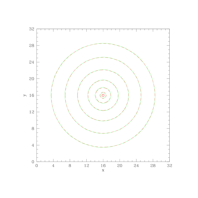
Figure 1: Distribution of flux in the x-y plane (with $z=16$) for a source sitting at cell (16,16,16) embedded in a static, uniform opacity distribution. The contour levels are logarithmically spaced with an increment of $1$ dex per contour level. The dashed contours are the analytic results (Equation 25) and solid contours are obtained with the present algorithm. The units for the contours levels are arbitrary.

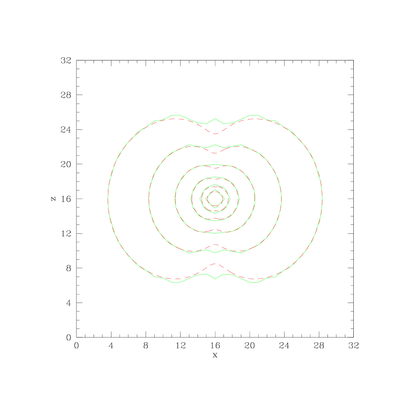
Figure 2: Distribution of flux in the x-z plane (with $y=16$) for a source sitting at cell (16,16,16) embedded in a static, elliptical opacity distribution (Equation 26). The contour levels are logarithmically spaced with an increment of $0.5$ dex per contour level. The dashed contours are the analytic results and solid contours are obtained with the present algorithm. The units for the contours levels are arbitrary.

3.2 Static Elliptical Optical Depth Distribution

The next step is to test a non-spherical static opacity distribution. An axisymmetric elliptical distribution of opacity of the following form is tested:

$$\kappa(\theta)={cb\over\sqrt{1-(1-b^{2})\cos^{2}\theta}},$$ (26)

where $\theta$ is the angle with respect to the positive $z$ direction, and $c$ and $b$ are the normalization and the ellipticity parameter of the distribution, respectively; $\kappa=c$ at $\cos\theta=1$ and $\kappa=cb$ at $\cos\theta=0$.

Figure 2 shows the computed flux distribution (solid contours) in the x-z plane with $y=16$ compared to the analytic result (dashed contours). We use $c=0.2$ and $b=0.2$ (see Equation 26) for this illustration. We see that the results are quite satisfactory given the Cartesian grid. The agreement with the analytic result is very good except near $\cos\theta=1$ where the opacity is the highest and a maximum error of 2 cells is made there. This is caused by a slight underestimate of the optical depth there, due to the averaging scheme of optical depth as indicated by Equations (23,24). We have also tested similar cases by varying either the opacity $c$ or ellipticity parameter $b$ (see Equation 26) and find that the results have similar accuracies.

3.3 Ionization of a Uniform Neutral Medium

We now switch to a higher gear to test the algorithm in a situation where the distribution of opacity changes self-consistently with time due to ionization. For this and subsequent tests we monitor photon number conservation by computing

$$\eta(t)={N_{e}(t)+N_{diff}(t)\over N_{ph,tot}(t)},$$ (27)

where $N_{e}(t)$ is the number of free electrons created by time $t$ (assuming 100% hydrogen) in the simulation box and $N_{diff}$ is the number of photons in the diffuse background in the simulation box volume at time $t$ and $N_{ph,tot}$ is the total number of photons emitted by time $t$ by sources in the simulation box. If photon number conservation is strictly observed, $\eta$ would be unity. In all the following tests recombination time is set to infinity to make the problem simple to track. But the accuracy of the method is unchanged by this simplification.

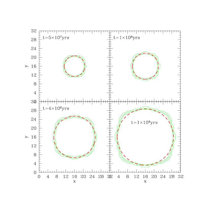
Figure 3: Distribution of neutral hydrogen fraction in the x-y plane (with $z=16$) for a source of luminosity $10^{51}~{}$photon/sec sitting at cell (16,16,16) in a uniform density $n=1\times 10^{-3}~{}$cm^-3 at four epochs $(5\times 10^{7},1\times 10^{8},4\times 10^{8},1\times 10^{9})~{}$yrs. The solid contours indicate the neutral hydrogen fraction of $0.3,0.6,0.9$ inside out computed with the present algorithm. The dashed contours are the radii from analytic calculations (Equation 28).

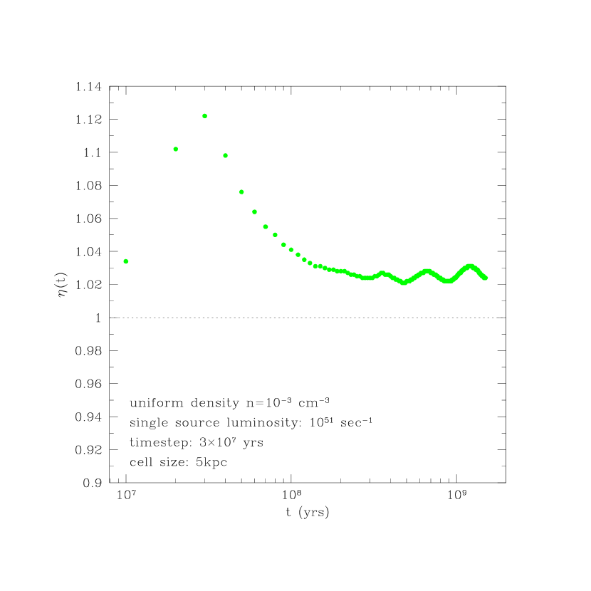
Figure 4: The error on photon number conservation (see Equation 27) as a function of time for the case of an ionizing galaxy surrounded by a uniform density distribution (see Figure 3).

We start with the case of a uniform neutral medium, consisting entirely of hydrogen atoms. An ionizing source of ionizing luminosity $\dot{N}_{ph}$ photon/sec is placed at cell $(16,16,16)$. The ionizing photons from the source ionize the neutral medium outward and the radius of the ionization front, the surface that separates the interior ionized medium from the exterior neutral medium, evolves with time approximately as:

$$r(t)=13.7({\dot{N}_{ph}\over 10^{51}})^{1/3}({n\over 10^{-3}{\rm cm^{-3}}})^{-1/3}({t\over 10^{7}{\rm yrs}})^{1/3}{\rm kpc},$$ (28)

where $n$ is the number density of the neutral hydrogen and $t$ is the elapsed time. The reason that this formula (26) is only approximate is that some photons may penetrate further out ahead of the ionization front, if the optical depth per cell is not sufficiently high, and then the “front” is no longer well defined; the formula would be highly accurate for a high opacity distribution. The optical depth per cell is $\tau_{\nu}=\sigma_{H}n\Delta x=15.4(n/10^{-3}{\rm cm^{-3}})(\Delta x/5{\rm kpc})$, where the hydrogen photo-ionization cross section $\sigma_{H}=10^{-18}~{}$cm² is used throughout and $\Delta x$ is the cell size. Thus, for the present test, the optical depth per cell is very large and formula (26) should be very accurate.

Figure 3 shows the contours of the neutral hydrogen fraction in the x-y plane with $z=16$ at four epochs. We use $\dot{N}_{ph}=10^{51}~{}$photon/sec, $n=10^{-3}~{}$cm^-3 and cell size of $\Delta x=5~{}$kpc. The adopted gas density is about 15 times the mean gas density at redshift $z=6$. We see that the agreement between the computed results and analytic expectations is excellent at all times. The discrepancy on the radius of the ionization front is evidently no larger than one cell. Given the approximations that have been made in the implementation, especially with respect to the computation of mean opacity (Equations 21,22), it is unclear how well the algorithm conserves photons. Figure 4 shows the degree of conservation of photons as a function of time. It is seen that, except for the first 8 time steps, the number of photons is conserved at better than $4\%$ with the average at about $2-3\%$. Timesteps of $10^{7}~{}$yrs are used but the results are insensitive to the timestep; using a timestep 3 times larger yield very similar results except for the upper left corner panel at the beginning of the simulation. Note that the age of the universe at $z=6$ is about $5\times 10^{8}~{}$yrs. The indicated convergence of results at this relatively large size of timesteps is clearly advantageous.

3.4 Ionization of an $r^{-1}$ Neutral Medium

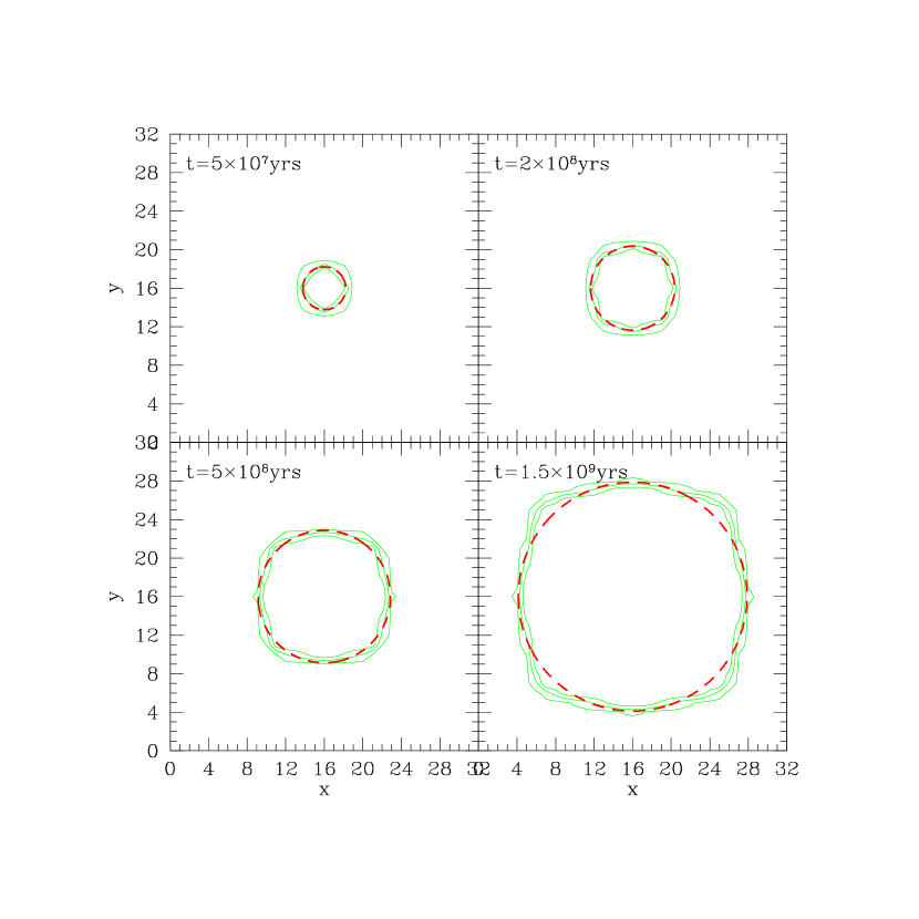
Figure 5: Distribution of neutral hydrogen fraction in the x-y plane (with $z=16$) for a source sitting at cell (16,16,16) in a density distribution of $n(r)\propto r^{-1}$ at four epochs $(5\times 10^{7},2\times 10^{8},5\times 10^{8},1.5\times 10^{9})~{}$yrs. The dashed contours are the analytic results (Equation 29) and solid contours are obtained with the present algorithm indicating the neutral hydrogen fractions of $0.3,0.6,0.9$ inside out.

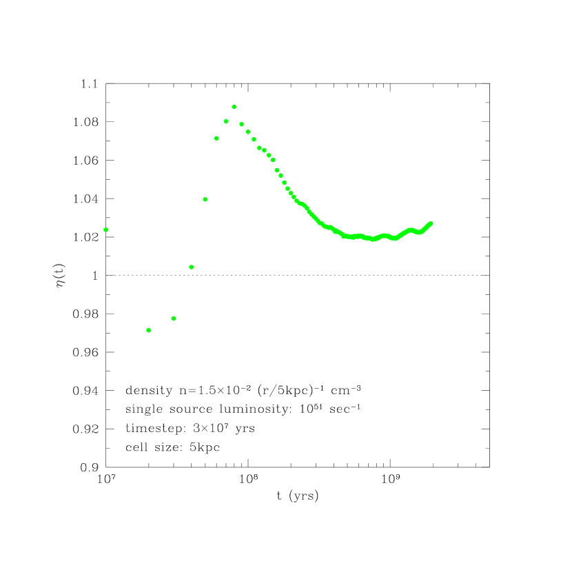
Figure 6: The error on photon number conservation as a function of time for the case of an ionizing galaxy surrounded by an $r^{-1}$ density distribution (see Figure 5).

Next, we examine a case of a source sitting in a spherical density distribution, $n=n_{c}(r/r_{c})^{-1}~{}$cm^-3; the central cell at $r=0$ is set to a density equal to $n_{c}(\Delta x/r_{c})^{-2}$, where $\Delta x$ is the cell size. This density profile is close to that in the central regions of dark matter halos (Navarro, Frenk, & White 1997) and is of significant cosmological relevance. The expected evolution of the radius of the ionization front is approximately:

$$r(t)=\sqrt{35.2({\dot{N}_{ph}\over 10^{51}{\rm sec^{-1}}})({n_{c}\over 10^{-2}{\rm cm^{-3}}})^{-1}({t\over 10^{7}{\rm yrs}})({r_{c}\over 5{\rm kpc}})^{-1}+25\left(({3\over 4\pi})^{2/3}-{1\over 2\pi}\right)\left({\Delta x\over 5{\rm kpc}}\right)^{2}}{\rm kpc},$$ (29)

where the second (correction) term inside the square root is due to the non-singular core of the modified $r^{-1}$ density distribution. The optical depth per cell as a function of source-centric radius is $\tau(r)=154(n/10^{-2}{\rm cm^{-3}})(\Delta x/5{\rm kpc})(r/r_{c})^{-1}$. Therefore, for the adopted values of $r_{c}$, $n_{c}$ and $\Delta x$ (see below), the formula will be very accurate over the range of radii examined and the thickness of the ionization front should be thin and close to one cell.

Figure 5 shows the contours of the neutral hydrogen fraction in the x-y plane with $z=16$ at four epochs. We use $\dot{N}_{ph}=10^{51}~{}$photon/sec, $n_{c}=1.5\times 10^{-2}~{}$cm^-3, $r_{c}=5~{}$kpc and cell size of $\Delta x=5~{}$kpc. Note that the adopted $n_{c}$ is approximately $200$ times the mean gas density at $z=6$. Timestep used is $10^{7}~{}$yrs but the results are insensitive to the timestep. From Figure 5 it is seen that the agreement between the computed results and analytic expectations is excellent at all times and the discrepancy on the radius of the ionization front is no larger than one cell. Figure 6 presents the degree of conservation of photons as a function of time, showing that the number of photons is conserved at better than $10\%$ with the average at about $2-3\%$ in this case.

3.5 Ionization of an $r^{-2}$ Neutral Medium

We turn to a steeper density distribution, $n=n_{c}(r/r_{c})^{-2}~{}$cm^-3; the central cell at $r=0$ is set to a density equal to $n_{c}(\Delta x/r_{c})^{-2}$, where $\Delta x$ is the cell size. The density profile is close to that of halos just interior of the virial radius (e.g., Tyson, Kochanski, & dell’Antonio 1998). The expected evolution of the radius of the ionization front is approximately:

$$r(t)=3.4({\dot{N}_{ph}\over 10^{51}})({n_{c}\over 10^{-2}{\rm cm^{-3}}})^{-1}({t\over 10^{7}{\rm yrs}})({r_{c}\over 5{\rm kpc}})^{-1}+5\left(({3\over 4\pi})^{1/3}-{1\over 4\pi}\right)({\Delta x\over 5{\rm kpc}}){\rm\ kpc},$$ (30)

where the second term on the right hand side is due to the non-singular core imposed on the density profile.

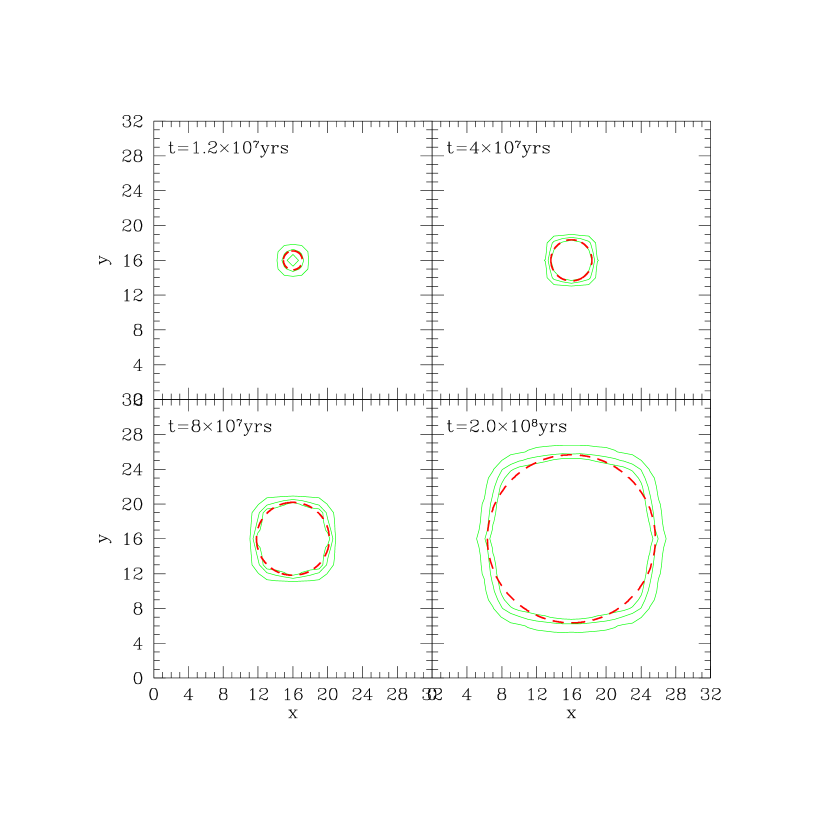
Figure 7: Distribution of neutral hydrogen fraction in the x-y plane (with $z=16$) for a source sitting at cell (16,16,16) in a density distribution of $n(r)\propto r^{-2}$ at four epochs $(1.2\times 10^{7},4\times 10^{7},8\times 10^{7},2\times 10^{8})~{}$yrs. The dashed contours are the analytic results (Equation 30) and solid contours are obtained with the present algorithm indicating the neutral hydrogen fractions of $0.3,0.6,0.9$ inside out.

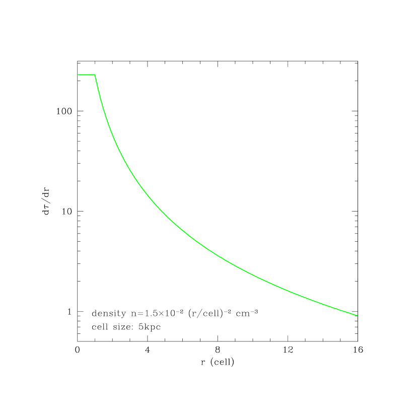
Figure 8: The original distribution of optical depth as a function of radius with an $r^{-2}$ density distribution. We see that at $r\geq 6$ cells a substantial amount of photons starts to penetrate outward ahead of the ionization front causing the slight thickening of the front, see in Figure 7.

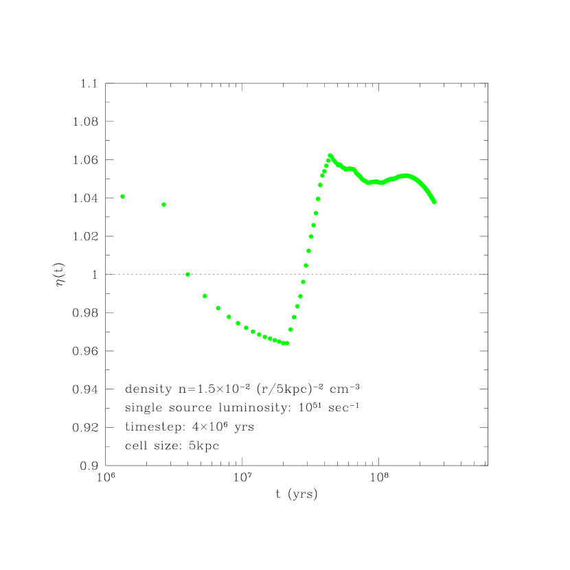
Figure 9: The error on photon number conservation as a function of time for the case of an ionizing galaxy surrounded by a $r^{-2}$ density distribution (see Figure 7).

Figure 7 shows the contours of the neutral hydrogen fraction in the x-y plane with $z=16$. We use $\dot{N}_{ph}=10^{51}~{}$photon/sec, $n_{c}=1.5\times 10^{-2}~{}$cm^-3, $r_{c}=5~{}$kpc and cell size of $\Delta x=5~{}$kpc at four epochs. Timestep used is $10^{7}~{}$yrs but like in other cases the results are insensitive to the timestep. The computed results and analytic expectations agree very well at all times. For the adopted values of $n_{c}$, $r_{c}$ and $\Delta x$, the optical depth per cell as a function of source-centric radius is $\tau(r)=154(n/10^{-2}{\rm cm^{-3}})(\Delta x/5{\rm kpc})(r/r_{c})^{-2}$ shown in Figure 8; we have $\tau(r)=3.6$ for $r=8~{}$cells. Thus, the computed shell of the ionization front will be somewhat broadened at late times due to a deeper penetration of ionizing photons outward of the ionization front, clearly evident in Figure 7. Figure 9 shows that the number of photons is conserved at better than $6\%$ with the average at about $1-4\%$ for this case.

3.6 Ionization of an Elliptical $r^{-2}$ Neutral Medium

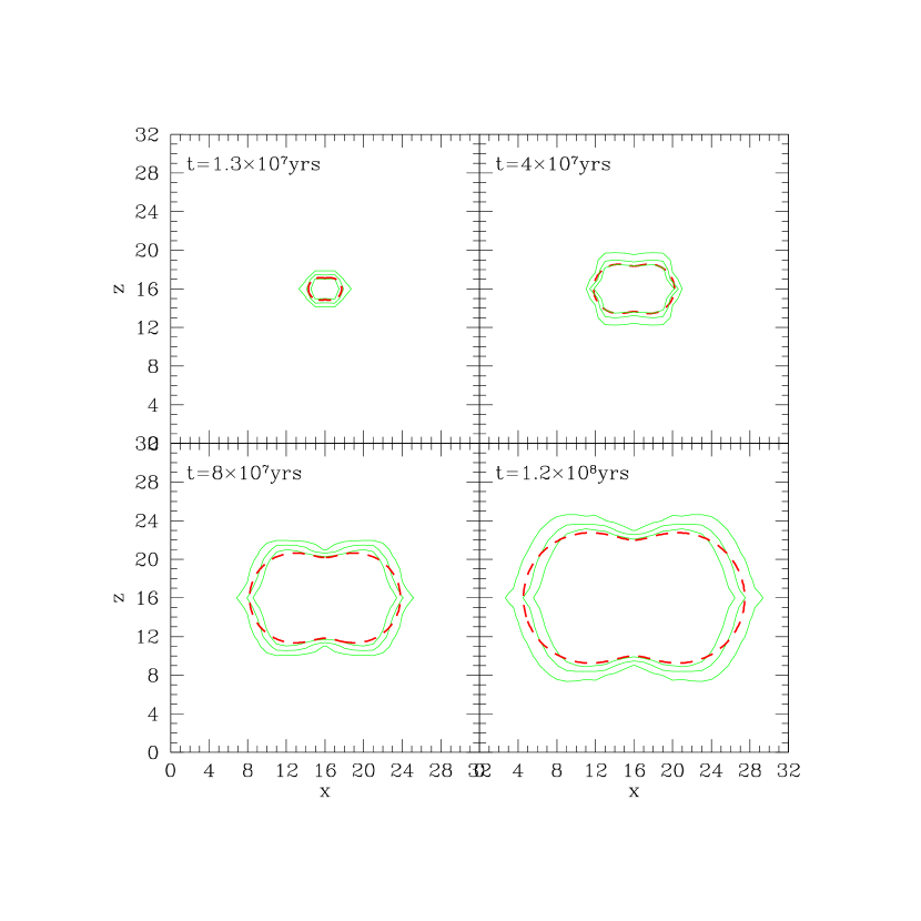
Figure 10: Distribution of neutral hydrogen fraction in the x-z plane (with $y=16$) for a source sitting at cell (16,16,16) in an elliptical isothermal density distribution of $n(r)\propto r^{-2}f(\theta)$ [see Equation 31 for the elliptical function of $f(\theta)$] at four epochs, $(1.3\times 10^{7},4\times 10^{7},8\times 10^{7},1.2\times 10^{8})~{}$yrs. The dashed contours are the analytic results and solid contours are obtained with the present algorithm, indicating the neutral hydrogen fractions of $0.3,0.6,0.9$ inside out.

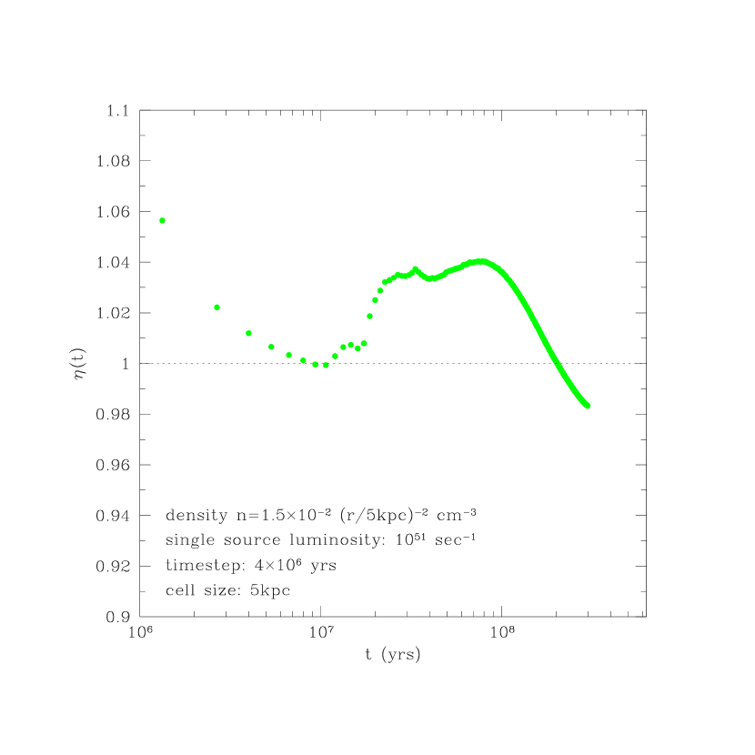
Figure 11: The error on photon number conservation as a function of time for the case of an ionizing galaxy surrounded an elliptical isothermal density distribution of $n(r)\propto r^{-2}f(\theta)$ (see Figure 10).

In realistic situations a source may sit inside a gas cloud that may not be spherical. We examine an elliptical isothermal distribution with the following density distribution

$$n(r,\theta)=n_{c}(r/r_{c})^{-2}{b\over\sqrt{1-(1-b^{2})\cos^{2}\theta}},$$ (31)

where $\theta$ is the angle with respect to the positive $z$ direction, and $b$ indicates the ellipticity of the distribution. The central cell at $r=0$ is designed not to be singular but has a density equal to $n_{c}(\Delta x/r_{c})^{-2}$, where $\Delta x$ is the cell size. The expected, orientation-dependent evolution of the radius of the ionization front follows Equation (30).

Figure 10 shows the contours of the neutral hydrogen fraction in the x-z plane with $y=16$ at four epochs. We use $\dot{N}_{ph}=10^{51}~{}$photon/sec, $n_{c}=1.5\times 10^{-2}~{}$cm^-3, $r_{c}=5~{}$kpc and cell size of $\Delta x=5~{}$kpc. Timestep used is $1.3\times 10^{6}~{}$yrs but the results are insensitive to the timestep. It is seen that the algorithm handles the anisotropic density distribution quite well and the agreement between the computed results and analytic expectations is very good at all times, with the computed ionization “fronts” tracing out the analytic results quite nicely with an error no larger than about one cell. The thickening of the computed “fronts” is real due to penetration of photons. Figure 11 shows the degree of conservation of photons. It is seen that the number of photons is conserved at better than $6\%$ with the average at about $1-4\%$.

3.7 Ionization of a Sharply Divided Anisotropic Neutral Medium

Figure 12: Distribution of neutral hydrogen fraction in the x-z plane (with $y=16$) for a source sitting at cell (16,16,16) embedded in a sharply divided anisotropic density field (see Equation 32) at four epochs $(2\times 10^{6},2\times 10^{7},4\times 10^{7},7.3\times 10^{7})~{}$yrs. The dashed contours are the analytic results and solid contours are obtained with the present algorithm, indicating the neutral hydrogen fractions of $0.3,0.6,0.9$ inside out.

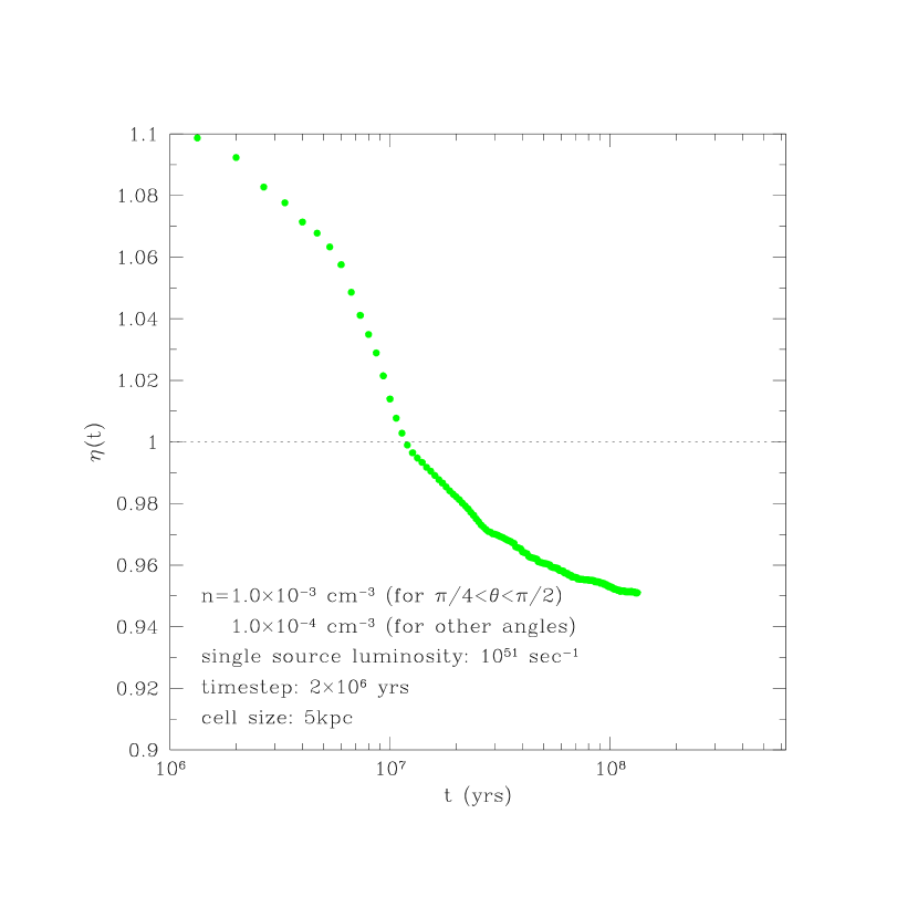
Figure 13: The error on photon number conservation as a function of time for the case of an ionizing galaxy surrounded by a sharply divided anisotropic density distribution (see Figure 12)

So far we have examined several different cases with smooth density distributions. It is prudent to test the algorithm in a more challenging situation. We pick a case where there are two different density fields separated by a sharp boundary. An axisymmetric density field is prescribed as

$$n(\theta) = 10^{-3}{\rm cm^{-3}}{\ \ \ \rm for\ {\pi\over 4}\leq\theta\leq{3\pi\over 4}}\hfill$$ (32)

$$= 10^{-4}{\rm cm^{-3}}{\ \ \ \rm otherwise.}\hfill$$

The source sits at cell $(16,16,16)$. The expected evolution of the radius of the ionization front follows Equation (28) for each of the two domains with different speeds of the ionization fronts.

Figure 12 shows the contours of the neutral hydrogen fraction in the x-z plane with $y=16$ at four epochs. We use $\dot{N}_{ph}=10^{51}~{}$photon/sec, $r_{c}=5~{}$kpc and cell size of $\Delta x=5~{}$kpc. Timestep used is $6.7\times 10^{5}~{}$yrs but the results are insensitive to the timestep. The agreement between the computed results and the analytic results are surprisingly good with the radius of the ionization front accurate to about one cell. At the boundaries separating the two regions there is a slight over-shielding on the low density side affected by the high optical depth, high density side. The width of this “affected” region is limited by the size of the solid angle of each discretized angular element, which in the present case is about $12^{2}$ square degrees. Figure 13 shows the degree of conservation of photons, indicating that the number of photons is conserved at better than $10\%$ with the average at about $1-5\%$.

3.8 Double Sources in a Uniform Density

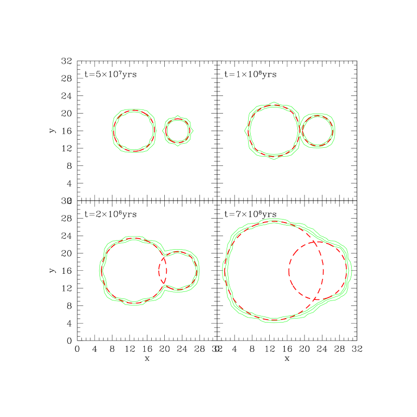
Figure 14: Distribution of ionization fraction in the x-y plane (with $z=16$) for two static sources sitting at cell (23,16,16) and cell (13,16,16) with luminosities of $\dot{N}_{ph}=2\times 10^{50}~{}$photon/sec and $\dot{N}_{ph}=10^{51}~{}$photon/sec, respectively, with a separation of $50~{}$kpc, at four epochs $(5\times 10^{7},1\times 10^{8},2\times 10^{8},7\times 10^{8})~{}$yrs. The dashed contours are the analytic results and solid contours are obtained with the present algorithm, indicating the neutral hydrogen fractions of $0.3,0.6,0.9$ inside out.

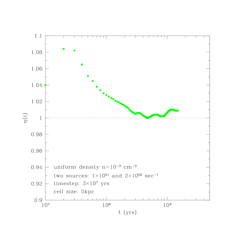
Figure 15: The error on photon conservation as a function of time for the case of two ionizing galaxies with luminosities of $10^{51}~{}$sec^-1 and $2\times 10^{50}~{}$sec^-1, respectively, separated by $50~{}$kpc surrounded by a uniform density distribution with $n=1\times 10^{-3}~{}$cm^-3.

Up to now we have tested cases with a single radiation source. It is important that the algorithm is capable of handling interactions of multiple radiation sources through the process of percolation, a process that is thought to occur during the cosmological reionization. We will demonstrate this by studying the situation where there are two sources of unequal luminosities. The two sources with luminosities $\dot{N}_{ph}=10^{51}~{}$photon/sec, and $2\times 10^{50}~{}$photon/sec, respectively, sit in a uniform neutral medium of density $n=10^{-3}~{}$cm^-3 initially. A cell size of $5~{}$kpc is used for the simulation box. The two sources are located at cell (23,16,16) and cell (13,16,16) with a separation of 10 cells (i.e., $50~{}$kpc). Timestep used is $10^{7}~{}$yrs but the results are insensitive to the size of the timestep.

Prior to the overlap of the two HII regions produced by the two sources separately, the evolution of each HII region is separate and the evolution of the radii of the ionization fronts follows Equation (28). Subsequent to the overlap their combined HII region will continue to expand but an analytic solution is not readily available. Figure 14 shows the contours of the neutral hydrogen fraction in the x-y plane with $z=16$ at four epochs. It is clear that the algorithm nicely treats the two separate regions without any interference before the overlap, with the two separate ionization fronts traveling at the correct speeds. For the post-overlap era we only show the analytic solution as if overlap has not occurred for the sole purpose of guiding the reader’s eye. The evolution of the ionization front in the post-overlap era is more complicated but the computed results appear to be quite reasonable, with the overlapped region continuing to expand and becoming rounder with time. In this case, one is more keen to check if the total number of photons is conserved. Figure 15 shows the degree of conservation of photons. It is seen the number of photons is conserved at better than $9\%$ with the average at about $1-2\%$.

3.9 Quadruple Sources in a Uniform Density

Let us make the situation a bit more interesting. We will add two more sources to the case tested in §3.8. The two additional sources have luminosities $\dot{N}_{ph}=3\times 10^{50}~{}$photon/sec, and $\dot{N}_{ph}=5\times 10^{50}~{}$photon/sec, sitting at cells (20,8,16) and (8,24,16) but turned on with lags of $1\times 10^{8}~{}$yrs and $2\times 10^{8}~{}$yrs (relative to the turn-on time of the initial two sources), respectively.

Figure 16 shows the contours of the neutral hydrogen fraction in the x-y plane with $z=16$ at four epochs. For the post-overlap era we only show the analytic solution as if overlap has not occurred for the sake of illustration. We see that the algorithm follows the separate HII regions, as expected. Continuous formation of galaxies in time can evidently be properly followed. Subsequent mergers of HII regions occur as expected. Figure 17 shows the degree of conservation of photons. It is seen the number of photons is conserved at better than $9\%$ with the average at about $1-3\%$. The evolution of the ionization front in the post-overlap era is very complicated but the computed results look reasonable, with the overlapped region continuing to expand in a fashion that is expected. The fact that photon number is well conserved and flux is designed to travel in the right direction ensures that the computed results should be accurate.

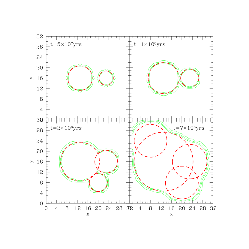
Figure 16: Distribution of neutral hydrogen fraction in the x-y plane (with $z=16$) at four epochs $(5\times 10^{7},1\times 10^{8},2\times 10^{8},7\times 10^{8})~{}$yrs. for four sources sitting at cells (23,16,16), (13,16,16), (20,8,16) and (8,24,16), with luminosities of $\dot{N}_{ph}=(2\times 10^{50},10^{51},3\times 10^{50},5\times 10^{50})~{}$ photon/sec, with turn-on times at $t=(0,0,1\times 10^{8},2\times 10^{8})~{}$yrs, respectively. The dashed contours are the analytic results (only valid times before the HII regions overlap) and solid contours are obtained with the present algorithm, indicating the neutral hydrogen fractions of $0.3,0.6,0.9$ inside out.

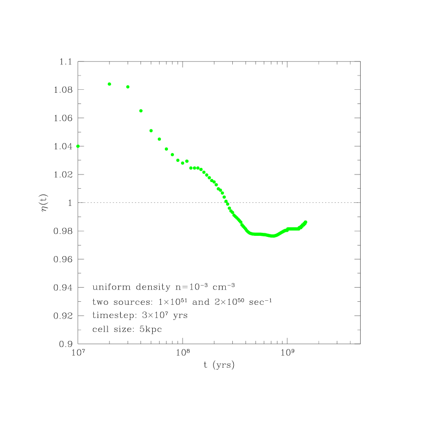
Figure 17: The error on photon number conservation as a function of time for the case of four ionizing galaxies with luminosities of $\dot{N}_{ph}=(2\times 10^{50},10^{51},3\times 10^{50},5\times 10^{50})~{}$ photon/sec, with turn-on times at $t=(0,0,1\times 10^{8},2\times 10^{8})~{}$yrs, respectively, surrounded by a uniform density distribution with $n=1\times 10^{-3}~{}$cm^-3 (see Figure 16).

3.10 Shadowing by a Dense Gas Cloud

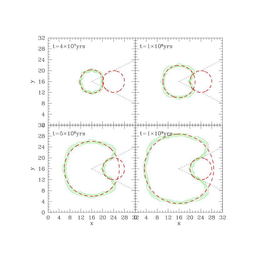
Figure 18: Distribution of neutral hydrogen fraction in the x-y plane (with $z=16$) for a source sitting at cell (16,16,16) of luminosity $10^{51}~{}$sec^-1 surrounded by a uniform density distribution with $n=1\times 10^{-3}~{}$cm^-3 at four epochs $(4\times 10^{7},1\times 10^{8},5\times 10^{8},1\times 10^{9})~{}$yrs. In addition, there is a spherical gas cloud of radius $20~{}$kpc centered at $(24,16,16)$ with a density distribution of $0.1(r/20{\rm kpc})^{-1}$. The small dashed circle on the right in each panel indicates the size of the halo. The (larger) dashed contours (on the left) are the analytic results and solid contours are obtained with the present algorithm, indicating the neutral hydrogen fractions of $0.3,0.6,0.9$ inside out. The analytic results are only valid before the ionization front reaches the halo; at subsequent times regions behind the halo delimited by the two dotted lines should remain neutral and the (large) circle on the left serves only to indicate the position of the ionization front if there were no obscuration.

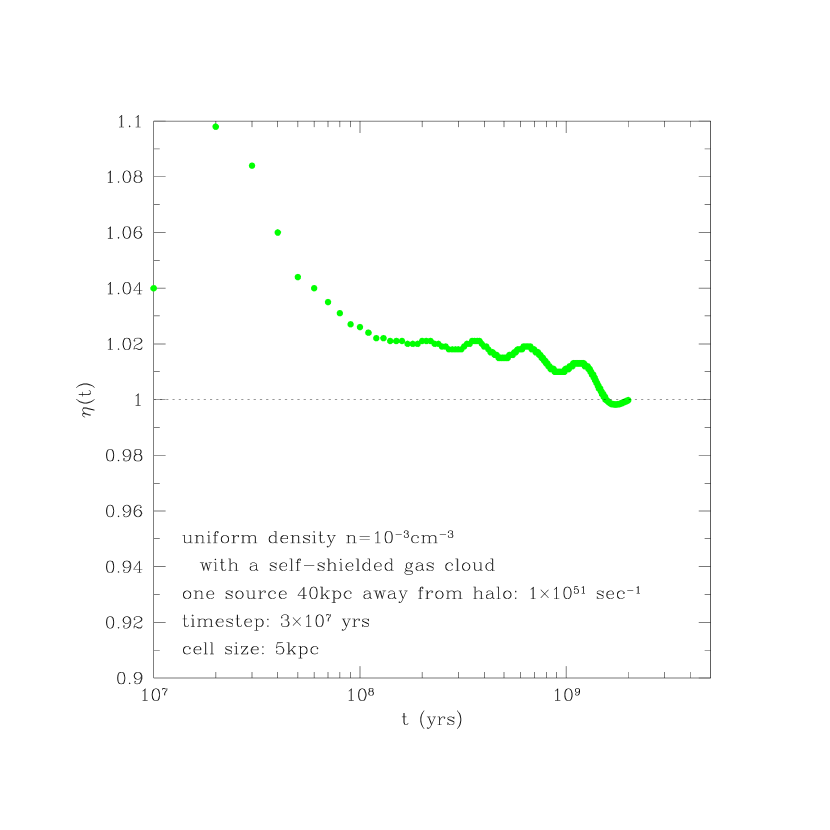
Figure 19: The error on photon number conservation as a function of time for the case of one ionizing galaxy with luminosity of $10^{51}~{}$sec^-1 surrounded by a uniform density distribution with $n=1\times 10^{-3}~{}$cm^-3. In addition, there is a spherical gas cloud of radius $20~{}$kpc centered at $(24,16,16)$ with a density distribution of $1\times 10^{-1}(r/20{\rm kpc})^{-1}$.

We will now step back to a case with a single source. But we will include in the uniform density field a dense gas cloud, which is designed to be optically thick to cast a shadow in the direction of radiation propagation. It is expected that shadowing should be common in the real universe since galaxies and other dense clouds (such as damped Lyman alpha systems) are (at least partially) opaque to radiation. A spherical gas cloud of radius $20~{}$kpc with a density distribution of $1\times 10^{-1}(r/20{\rm kpc})^{-1}~{}$cm^-3 is centered at cell $(24,16,16)$. The rest of the simulation box has a uniform density of $1\times 10^{-3}~{}$cm^-3. The ionizing source is located at cell (16,16,16) with a luminosity of $10^{51}~{}$sec^-1. A cell size of $\Delta x=5~{}$kpc is used for the simulation. Figure 18 shows the neutral hydrogen fraction contours at four epochs. The analytic results are only valid before the ionization front reaches the halo; at subsequent times regions behind the halo within the region delimited by the two dotted lines should remain neutral. We indeed see the shadow cast by the dense gas cloud. The slightly overshadowing near the edges of the shadowed region is due to the limited resolution of angular discretization, also seen in Figure 12.

The relatively complicated situation here does not guarantee that photon number conservation will be obeyed. Figure 19 shows the degree of conservation of photons. Quite reassuringly, we see that the number of photons is conserved at better than $10\%$ with the average at about $1-2\%$.

3.11 Outside-In Ionization of a Spherical Isothermal Gas Cloud

Let us next examine another class of ionization processes, where external diffuse radiation ionizes isolated overdense regions. This type of ionization process is common in cosmological situations where low density regions become ionized first. In this case we check the photon number conservation in a slightly different way as:

$$\eta(t)={N_{e}(t)\over N_{incoming}(t)},$$ (33)

where $N_{e}(t)$ is the number of free electrons created by time $t$ in the simulation box and $N_{incoming}$ is the number of incoming photons from the diffuse background that are absorbed in the simulation box volume by time $t$. If photon number conservation is strictly observed, $\eta$ would be unity. Recombination time is set to infinity.

The first simple example is the ionization of a spherical isothermal gas cloud of density $n=n_{c}(r/r_{c})^{-2}~{}$cm^-3 with an outer cutoff radius $r_{i}$; the central cell at $r=0$ has a density equal to $n_{c}(\Delta x/r_{c})^{-2}$ to avoid singularity, where $\Delta x$ is the cell size. The expected evolution of the radius of the ionization front, which now travels inward towards the center of the gas cloud, is approximately:

$$r(t)={r_{i}n_{c}r_{c}^{2}\over 0.5Fr_{i}t+n_{c}r_{c}^{2}},$$ (34)

where $F$ is the diffuse flux assumed to be constant with time. Note that the factor $0.5$ in front of flux $F$ in Equation (34) is due to the fact that any element on the surface is subject to radiation only at half the total solid angle.

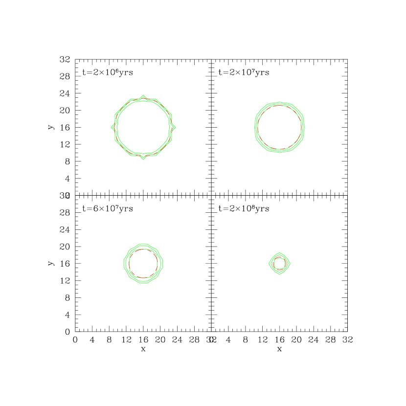
Figure 20: Distribution of neutral hydrogen fraction in the x-y plane (with $z=16$) for an isothermal gas cloud sitting at cell (16,16,16), exposed to an external isotropic diffuse radiation background, at four epochs $(2\times 10^{6},2\times 10^{7},6\times 10^{7},2\times 10^{8})~{}$yrs. The dashed contours are the analytic results (Equation 34) and solid contours are obtained with the present algorithm. indicating the neutral hydrogen fractions of $0.3,0.6,0.9$ outside in.

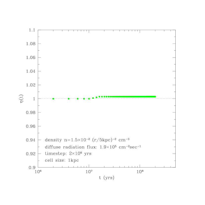
Figure 21: The error on photon number conservation as a function of time for the case of a halo of density $n_{c}=1.5\times 10^{-2}(r/5{\rm kpc})^{-2}~{}$cm^-3, subject to a diffuse background flux of $19\times 10^{5}~{}$cm^-2sec^-1.

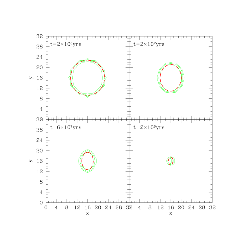
Figure 22: Distribution of neutral hydrogen fraction in the x-z plane with $y=16$ for an elliptical isothermal gas cloud (see Equation 35) sitting at cell (16,16,16), exposed to an external isotropic diffuse radiation background, at four epochs $(2\times 10^{6},2\times 10^{7},6\times 10^{7},2\times 10^{8})~{}$yrs. The dashed contours are the analytic results and solid contours are obtained with the present algorithm, indicating the neutral hydrogen fractions of $0.3,0.6,0.9$ outside in.

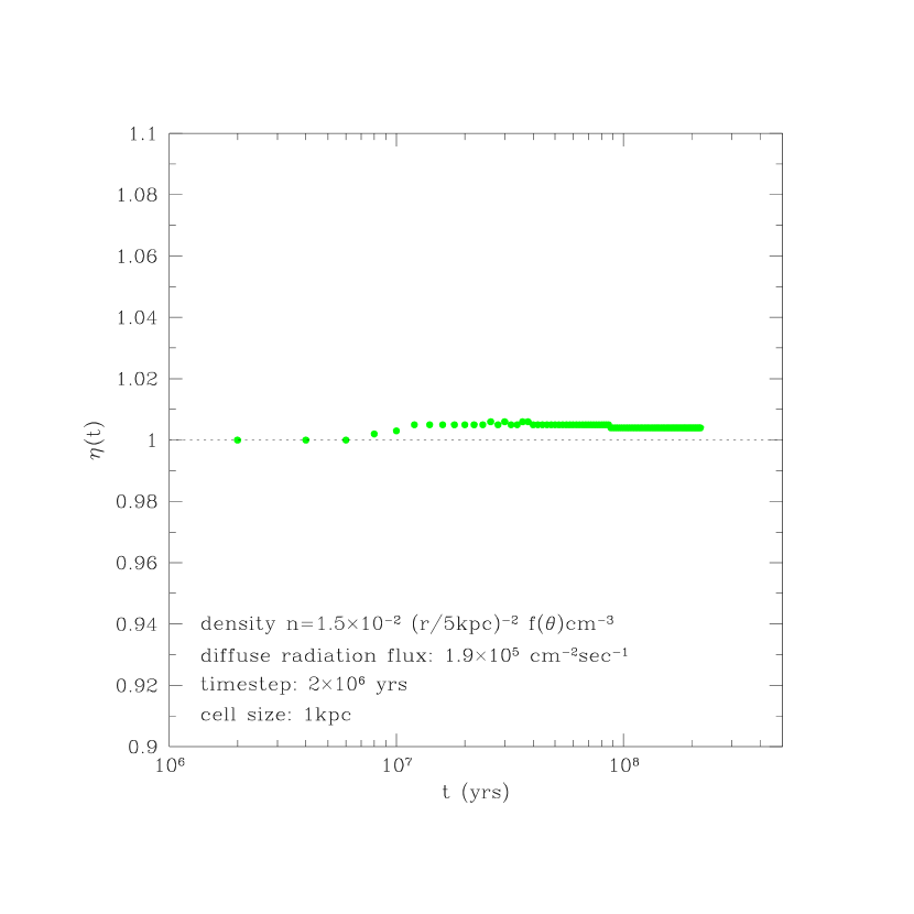
Figure 23: The error on photon number conservation as a function of time for the case of an elliptical isothermal gas cloud (see Equation 35) sitting at cell (16,16,16), exposed to an external isotropic diffuse radiation background.

Figure 20 shows the evolution of the ionization front in the x-y plane with $z=16$. We use $r_{c}=5~{}$kpc, $n_{c}=1.5\times 10^{-2}$, $\Delta x=1~{}$kpc, $b=0.5$ and $F=1.9\times 10^{5}~{}$cm^-2sec^-1. We see that the analytic evolution of the ionization front is well tracked by the computed results with error on the radius no larger than one cell. The spiky surface at the earliest time shown reflects the initial condition laid out on a Cartesian grid. Figure 21 shows the photon number conservation as a function of time and again indicates that the method conserves total number of photons very well at $<1\%$. The high degree of photon conservation in case is attributable to the fact that there is no obscuration for the cells on the ionization surface that receive ionizing photons.

3.12 Outside-In Ionization of an Elliptical Isothermal Gas Cloud

We next consider ionization of an isolated elliptical isothermal gas cloud of the following density profile by a diffuse ionizing background

$$n(r,\theta)=n_{c}(r/r_{c})^{-2}{b\over\sqrt{1-(1-b^{2})\cos^{2}\theta}};$$ (35)

the central cell at $r=0$ has a density equal to $n_{c}(\Delta x/r_{c})^{-2}$ to avoid singularity, where $\Delta x$ is the cell size. The expected evolution of the radius of the ionization front follows Equation (34) with an angle-dependent $n_{c}$ indicated by Equation (35).

Figure 22 shows the evolution of the ionization front in the x-z plane with $y=16$. We use $r_{c}=5~{}$kpc, $n_{c}=1.5\times 10^{-2}$, $\Delta x=1~{}$kpc and $F=1.9\times 10^{5}~{}$cm^-2sec^-1. We see that the analytic evolution of the ionization front is well traced by the computed results with error on the radius no larger than one cell. Figure 23 shows the photon number conservation as a function of time and again indicates that the method conserves total number of photons very well at $<1\%$.

3.13 Radiation Propagation In a Realistic Cosmological Density Field

Finally, we turn to the radiation propagation in a realistic density field produced by cosmological simulations. In this case, the situation is much more complicated and no analytic solution is possible. But many of the cases tested above have significant bearings on this realistic case. We take a subbox from one of our latest simulations (Cen et al. 2001) at redshift $z=6$. The subbox has a $32^{3}$ grid and a cell size of $4.65~{}$kpc proper.

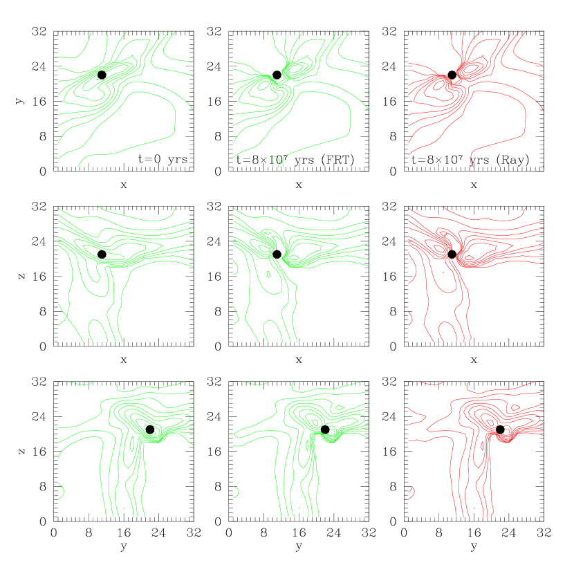
Figure 24: The left column shows projected gas density fields along three faces of the box (three rows) for a three-dimensional box with $32^{3}$ grid points and a cell size of $4.65~{}$kpc proper at the initial time. The solid dot indicates the position of the putative galaxy of luminosity $10^{51}~{}$sec^-1. The contours are: the first contour is at the mean density and subsequent ones increase by 0.2 dex per contour. The middle column shows projected neutral hydrogen density fields along three faces of the box at $t=8\times 10^{7}$yrs, computed with the present method. The right column shows projected neutral hydrogen density fields along three faces of the box at $t=8\times 10^{7}$yrs, computed using a high resolution ray tracing code (with 38416 rays from the source).

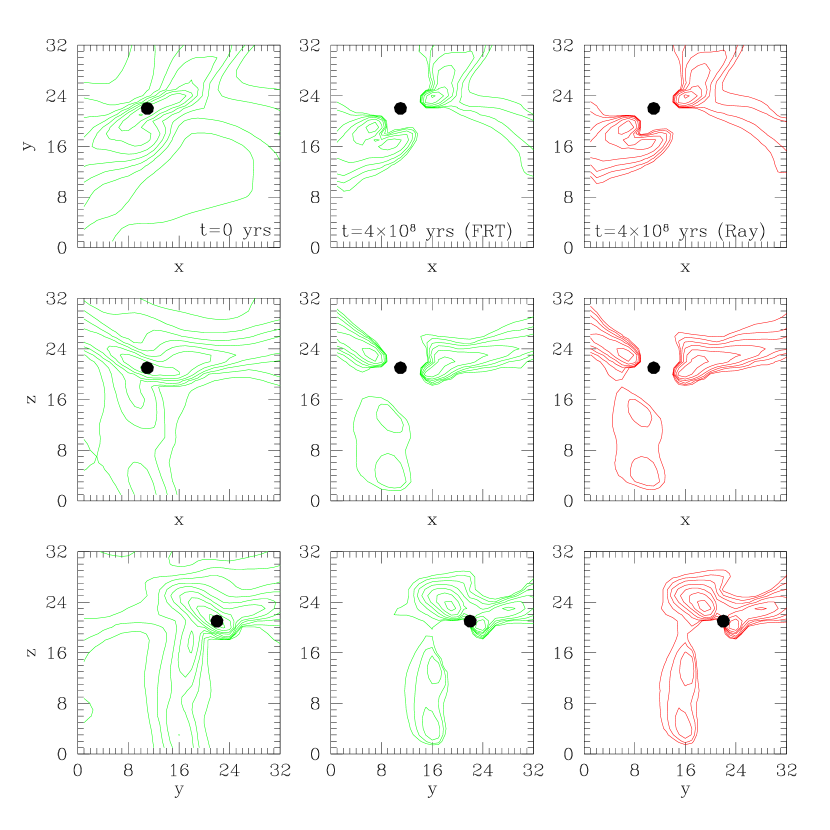
Figure 25: The left column shows projected gas density fields along three faces of the box (three rows) for a three-dimensional box with $32^{3}$ grid points and a cell size of $4.65~{}$kpc proper at the initial time. The solid dot indicates the position of the putative galaxy of luminosity $10^{51}~{}$sec^-1. The contours are: the first contour is at the mean density and subsequent ones increase by 0.2 dex per contour. The middle column shows projected neutral hydrogen density fields along three faces of the box at $t=4\times 10^{8}$yrs, computed with the present method. The right column shows projected neutral hydrogen density fields along three faces of the box at $t=4\times 10^{8}$yrs, computed using a high resolution ray tracing code (with 38416 rays from the source).

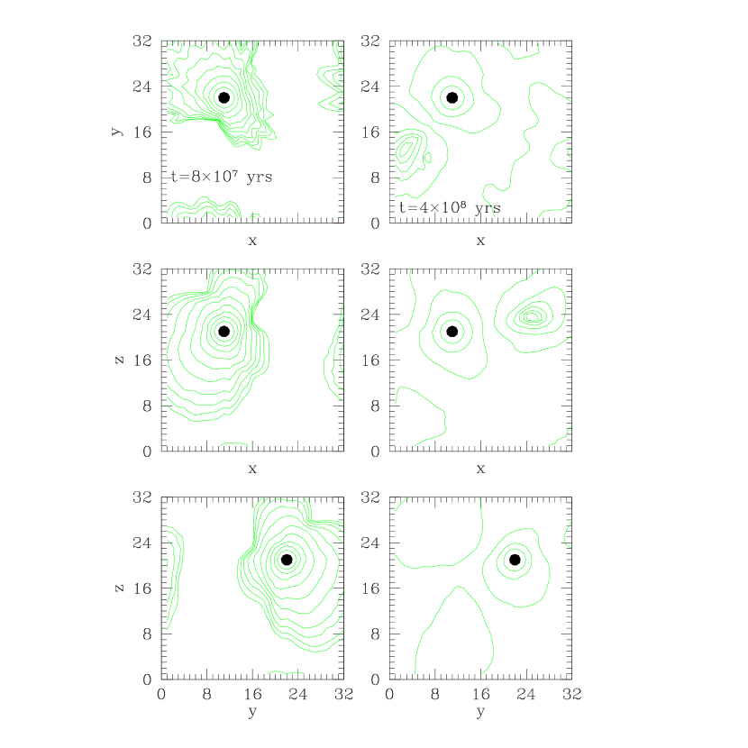
Figure 26: Volume-weighted flux distributions projected along three faces of the box at the two times, $t=(8\times 10^{7},4\times 10^{8})$yrs, shown in Figure 24 and Figure 25, respectively. The first contour around the solid dot (the galaxy) has a flux of $10^{8.5}$cm^-2sec^-1 and the decrement for the successive contours is 0.25 dex.

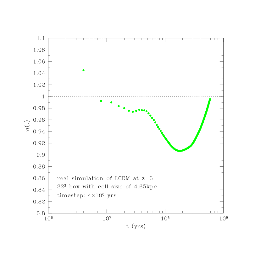
Figure 27: The error on photon number conservation as a function of time for the case of ionization of a realistic density field produced in cosmological simulations at $z=6$.

We turn on by hand a galaxy of ionizing luminosity of $\dot{N}_{ph}=10^{51}~{}$sec^-1 at cell $(11,22,21)$ corresponding to the densest cell in the box, as indicated by the solid dot in Figures (24,25,26). We assume that the gas is composed entirely of hydrogen and at the starting time hydrogen is entirely neutral. For simplicity we have set the recombination time to infinity. It is noted that the galaxy sits in a generic filament, which is embedded in a complex structure containing voids and other interesting structures. Since the subbox is a small region of a large, periodic box, it is not periodic itself. But we treat it as if it were periodic.

Figure 24 and Figure 25 show the distribution of neutral hydrogen at time $t=(8\times 10^{7},4\times 10^{8})$yrs (middle columns), respectively, compared to that at the starting time ($t=0$; left column). The most notable feature is that the radiation propagation is highly anisotropic. The ionizing photons quickly clear out widening tunnels towards low density (void) regions in the direction perpendicular to the filament, while radiation front travels at much slower speeds in other directions. Although this is not at all surprising, the figures do remind us of the complex situations encountered in cosmological structures and re-iterate the need for a proper treatment of radiative transfer. We also use a high resolution ray tracing code to obtain numerically the approximate “true” distribution, shown as the right columns. Note that in the ray tracing code one just counts photons and compares to the number of hydrogen atoms along each ray cone; photon penetration ahead of the ionization front is not taken into account and ionization front is taken to be abruptly sharp. Nevertheless, the results obtained with the ray tracing method should be fairly close to the ‘truth”. We see that the agreement between the result obtained with the present method and that with the ray tracing method is excellent.

Figure 26 shows the projected flux distributions (volume-weighted) at the two epochs respectively. We see that flux distributions are quite complex but consistent with the neutral hydrogen distributions. It is seen at the earlier epoch, when substantial blocking or shadowing exists, the contours of the flux distribution tend to orient perpendicular to the contours of the neutral hydrogen density. Note that in the present calculations we have set the recombination time to infinity; in a more involved calculation including recombination it is expected that fluctuations in the flux distributions would be enhanced.

Finally, Figure 27 shows how the total number of photons is conserved. We are once again seeing satisfactory conservation of photons in this realistic simulation at about $1-10\%$ level with a time averaged accuracy of $3-5\%$. This level of photon number conservation is quite adequate for cosmological simulations, since other uncertainties, including galaxy luminosity, radiation escape fraction from the galaxies, star formation efficiency, etc., are usually much larger. Besides, we expect that we may be able to improve the accuracy of the algorithm by more detailed experimenting and careful fine tuning, if necessary.

The fact that photon number is well conserved and flux is designed under the algorithm to propagate in the right directions guarantee that the results should be reliable, as verified by the comparison with the results from a high resolution ray tracing method.

3.14 Summary on the Tests

We have performed a variety of tests on the proposed algorithm for transferring radiation in three dimensional space. The tests are designed to be relevant to cosmological applications. It is worthwhile to re-emphasize that the proposed algorithm, by design, guarantees that flux propagates in the right direction in any situation. Thus, the tests should mainly demonstrate how accurately the amplitude of the flux is computed.

To summarize the results we find, the flux is computed very accurately, resulting in ionization fronts that travel at the correct speed with error no larger than one cell in all cases. Photon number is conserved with a maximum error of about $10\%$ and an average error of $1-5\%$ over hundreds of time steps for all the cases tested, with $m_{a}=256$ angular elements and $m_{r}=18$ logarithmically spaced radial bins on a $32^{3}$ grid. We note that in the limit of infinite values for $m_{r}$ and $m_{a}$, the present method solves the equation of the radiative transfer exactly and the approximation would represent the truth. In other words, the tests have basically shown that with reasonable number of angular and radial discretization elements the proposed method gives quite accurate results.

Finally, we find that the accuracy of the algorithm does not depend sensitively on the time step used. A time step of size comparable to the typical time step in cosmological hydrodynamic simulations appears sufficient. This feature is desirable with regard to the overall computational cost.

4 Discussion and Conclusions

In light of the recent observations of high redshift quasars (e.g., Fan et al. 2001), indicating that the cosmological reionization may be just ending at redshift $z\sim 6$ (Becker et al. 2001; Barkana 2001; Cen & McDonald 2001), a new and exciting frontier is forming. Inhomogeneous reionization of the universe is now within the observational reach and could potentially provide a great tool to test both cosmological models and astrophysics of galaxy formation (e.g., Barkana & Loeb 2001). It has thus become mandatory to perform cosmological hydrodynamic simulations that tackle this problem with an adequate treatment of radiative transfer. Furthermore, even in the post-reionization era, an initial inhomogeneous reionization process coupled with the significant clustering of radiation sources (galaxies or quasars) as well as the fluctuating density field likely produces fluctuations both in the thermodynamic properties of the cosmic gas and in the ionizing radiation field. Such fluctuations may substantially alter quantitatively (or even qualitatively) the picture of the optically thin regions of the Ly$\alpha$ forest on a variety of scales, which would limit our ability of accurately extracting important cosmological information from observations of the Ly$\alpha$ forest. Lastly (but not the least), since almost all neutral gas resides and star formation occurs only in dense, optically thick regions, many questions pertaining neutral gas and star formation in the universe can be answered with confidence only when radiative transfer is properly included.

We have developed a fast, accurate and robust algorithm for radiative transfer in three-dimensional space. The core of the algorithm is based on a formulation that the summation of any quantity (such as emissivity or opacity) over any volume can be written in the standard convolution form, which can be computed efficiently using the Fast Fourier Transform techniques. We will name this method “FRT” (Fast Radiative Transfer) method. The overall computational time with this algorithm scales as $N(\log N)^{2}$, where $N$ is the number of grid points in a simulation box. Therefore, this is a fast algorithm. We stress that the computational cost with this method is independent of the number of radiation sources, providing a natural match to cosmological simulations where a large number of sources are present. Local sources and diffuse background are naturally split and the evolution of each of the two components as well as interactions between them are handled self-consistently. The devised integral form of the algorithm guarantees that the method is completely stable and robust.

The algorithm is tested on a wide range of analytically tractable problems that have significant bearings on cosmological applications. We find that the algorithm performs very well in all cases, accurately tracking ionization fronts with the error no larger than one cell. Conservation of photons is observed to be at a level of a few percent. The accuracy of the results depends weakly on the size of the time step in all cases; a time step comparable to the typical size of a time step for a cosmological hydrodynamic simulation is sufficient. We also apply the algorithm to a realistic density field produced by a cosmological hydrodynamic simulation and find that conservation of photons is observed at a level of a few percent. These extensive tests indicate that the algorithm is also very accurate.

The tests performed is based on a first implementation of the basic algorithm outlined in the paper. It is clear that there is significant room for further improvement over the specific implementation. The current implementation is on a uniform mesh but we think that variant approaches (such as with adaptive mesh refinement, for example) based on this method are possible and will be explored in the future.

References

- Abell (1958) Abel, T., Norman, M.L., Madau, P. 1999, ApJ, 523, 66
- Abell (1958) Barkana, R., 2001, astro-ph/0108431
- Abell (1958) Barkana, R., & Loeb, A. 2001, Phys. Rep., 349, 125
- Abell (1958) Barnes, J., & Hut, P. 1986, Nature, 324, 446
- Abell (1958) Becker, R.H., et al. 2001, astro-ph/0108097
- Abell (1958) Cen, R., Miralda-Escudé, J., Ostriker, J. P., & Rauch, M. 1994, ApJ, 437, L9
- Abell (1958) Cen, R., & McDonald, P. 2001, astro-ph/0110306, ApJ, in press
- Abell (1958) Cen, R., & Ostriker, J.P. 1993, ApJ, 417, 404
- Abell (1958) Cen, R., & Ostriker, J.P. 1999, ApJ, 514, 1
- Abell (1958) Cen, R., Tripp, T.M., Ostriker, J.P., & Jenkins, E.B. 2001, ApJ, 559. L5
- Abell (1958) Ciardi, B., Ferrara, A., Marri, S., Raimondo, G. 2001, MNRAS, 324, 381
- Abell (1958) Croft, R.A.C., Weinberg, D.H., Katz, N., & Hernquist, L. 1998, ApJ, 495, 44
- Abell (1958) Fan, X., et al. 2001, astro-ph/0108063
- Gnedin & Ostriker (1997) Gnedin, N.Y., & Ostriker, J.P. 1997, 486, 581
- Abell (1958) Hernquist, L., Katz, N., Weinberg, D.H., & Miralda-Escudé 1996, ApJ, 457, L51
- Abell (1958) Kessel-Deynet, O., & Burkert, A. 2000, MNRAS, 315, 713
- Abell (1958) Miralda-Escudé, J., Cen, R., Ostriker, J. P., & Rauch, M. 1996, ApJ, 471, 582
- Abell (1958) Navarro, J.F., Frenk, C.S., & White, S.D.M. 1997, ApJ, 490, 493
- Abell (1958) Norman, M.L., Paschos, P., & Abel, T. 1998, MmSAI, 69, 455
- Abell (1958) Razoumov, A.O., Scott, D. 1999, MNRAS, 309, 287
- Abell (1958) Sokasian, A., Abel, T., & Hernquist, L. 2001, NewA, submitted, astro-ph/0105181
- Abell (1958) Stone, J.M., Mihalas, D., & Norman, M.L. 1992, ApJS, 80, 819
- Abell (1958) Tyson, J.A., Kochanski, G.P., & dell’Antonio, I.P. 1998, ApJ, 498, L107
- Abell (1958) Zhang, Y., Anninos, P., & Norman, M.L. 1995, ApJ, 453, L57