Modified Median Statistics and Type Ia Supernova Data

Abstract

The median statistic has recently been discussed by Gott et al. as a more reliable alternative to the standard $\chi^{2}$ likelihood analysis, in the sense of requiring fewer assumptions about the data and being almost as constraining. We apply this statistic to the currently available combined dataset of 92 distant type Ia supernovae, and also to a mock SNAP-class dataset. We find that the performances of the modified median and $\chi^{2}$ statistics are comparable, particularly in the latter case. We further extend the work of Gott et al. by modifying the median statistic to account for the number and size of sequences of consecutive points above or below the median. We also comment on how the performance of the statistic depends on the choice of free parameters that one is estimating.

1 Introduction

In recent work Gott et al. (2001) have argued, through several convincing examples, that the median statistic is a reliable alternative to the usual $\chi^{2}$ likelihood analysis. Even though it usually has the caveat of not being as constraining (for the same data set), it has the strong advantage of requiring much weaker assumptions about the dataset itself and its errors. Furthermore, it is also less vulnerable than the mean to the presence of bad data, such as when ‘outliers’ exist. Hence, if nothing else, median statistics can be useful for the early stages of a data analysis pipeline, when one is still trying to put together evidence that may justify the use of stronger hypotheses on the dataset.

In this work, we apply the median statistic to the combined dataset of 92 type Ia supernovae taken from the Supernova Cosmology Project (SCP) (Perlmutter et al., 1999) and the High-z Supernova Search Team (HzST) (Riess et al., 1998). This is a particularly relevant example, since the current data set is still fairly small. Furthermore, the physics of supernova explosions is not at all well known, and hence the possible presence of outliers in the available data is a particular concern.

We also apply our results to a SNAP-class (Nugent, 2000; Weller & Albrecht, 2001) simulated dataset. We further extend the analysis of Gott et al. (2001) by considering simple modifications of the median statistic which account for the number and size of sequences of consecutive points above or below the median (to which the standard median statistic is ‘blind’). We discuss the dependence of the performance of the statistic on the choice of free parameters that one is estimating and we find that the median statistic can be competitive with the standard $\chi^{2}$ analysis, provided one knows the Hubble parameter $H_{0}$ (or equivalently the absolute magnitude of a standard type Ia supernova).

The rest of the paper is organised as follows. In Section 2 we briefly recall the tools necessary to carry out the estimation of the present day values of the cosmological parameters $\Omega_{m}$ and $\Omega_{\Lambda}$ from a type Ia supernova dataset. In Section 3 we introduce the median statistic as a data analysis method and motivate some simple modifications thereof. We then present our results in Section 4, and finally in Section 5 we draw some conclusions and discuss possible further improvements.

2 Cosmological parameters from type Ia supernovae

Following the release of the results from the Supernova Cosmology Project (SCP) (Perlmutter et al., 1999) and the High-z Supernova Search Team (HzST) (Riess et al., 1998), which altogether include some 100 supernovae, there has been an increased effort towards the parameterisation of the energy content of the Universe using Type Ia Supernovae (Weller & Albrecht, 2001).

The currently available data, when combined with CMB results (Jaffe et al., 2001) indicates that about one third of the critical energy density in the Universe is in the form of ordinary matter (and here we include the classic dark matter), while the remaining two thirds are in the form of a so-called dark energy component, the exact form of which is yet unknown. The cosmological constant $\Lambda$ is arguably the simplest candidate for this dark energy (Bean & Melchiorri, 2002), though there are various other contenders, from frustrated topological defects (Bucher, 1999) to a time varying cosmological constant (Peebles & Ratra, 1988; Ratra & Peebles, 1988; Podariu & Ratra, 2000; Waga & Frieman, 2000), in particular what is commonly called quintessence (Caldwell, Dave, & Steinhardt, 1998; Wang et al., 2000). The main problem associated with the cosmological constant is that theoretical predictions of its value are many orders of magnitude off from the experimental results (Carroll, Press & Turner, 1992). On the other hand, quintessence may suffer from considerable ‘coincidence’ problems.

Aiming to help settling the question of the constitution of dark energy, the SNAP (Supernova Acceleration Probe) (Nugent, 2000) satellite was recently proposed. Its goal is to obtain a supernova dataset more than one order of magnitude larger than currently available datasets, with much-improved control over systematic errors, to redshifts up to about $z\simeq 1.7$. Even though SNAP results are still years away, we can of course simulate the expected results, and thus forecast the impact of this improved dataset on the constraints on the energy density and equation of state of dark energy that permeates the Universe (Weller & Albrecht, 2001).

As usual, the parameter fit is done through the luminosity distance $d_{L}$, defined as

$${\mathcal{F}}=\frac{{\mathcal{L}}}{4\pi d_{L}{}^{2}}\,,$$ (1)

where ${\mathcal{L}}$ is the intrinsic luminosity of the source and ${\mathcal{F}}$ the measured flux. From the Friedmann–Robertson–Walker metric it follows that this distance is given, as a function of redshift $z$, by

$$d_{L}=\frac{c(1+z)}{H_{0}\sqrt{|\Omega_{k}|}}\ S(\sqrt{|\Omega_{k}|}\int_{0}^{z}(\Omega_{m}(z^{\prime}+1)^{3}+\Omega_{\Lambda}+(z^{\prime}+1)^{2}\Omega_{k})^{-\frac{1}{2}}dz^{\prime})\,,$$ (2)

where $\Omega_{k}=1-\Omega_{m}-\Omega_{\Lambda}$, and the function $S$ is defined as

$$S(x)=\left\{\begin{array}[]{ll}\sin x,&\Omega_{k}<0\\ x,&\Omega_{k}=0\\ \sinh x,&\Omega_{k}>0\end{array}\right.\,.$$ (3)

The apparent magnitude $m$ of a supernova (a parameter more often used than the measured flux ${\mathcal{F}}$, to which it is related) at a given redshift is then given by

$$m=M+5\log\left(\frac{d_{L}}{{\rm{Mpc}}}\right)+25\,,$$ (4)

$M$ being the absolute magnitude of the supernova (related to its intrinsic luminosity ${\mathcal{L}}$). Following Wang (Wang et al., 2000), we use results from both the SCP and HzST even though their published datasets differ in presentation. We define the distance modulus

$$\mu_{0}=5\log\left(\frac{d_{L}}{{\rm{Mpc}}}\right)+25\,,$$ (5)

as presented in the HzST results comprising 50 supernovae. Comparatively, the SCP published the estimated effective B-band magnitude $m_{b}^{\textrm{eff}}$ for 60 supernovae which relates to the HzST results through

$$m_{B}^{\textrm{eff}}=M_{B}+\mu_{0}\,,$$ (6)

where $M_{B}$ is the peak B-band absolute magnitude of a standard type Ia supernova. The published results of the SCP and HzST groups have 18 common supernovae, 16 of which are from the Calán–Tololo Survey data (Phillips et al., 1999). If we calculate $M_{B}$ by comparing results for these 18 supernovae (using the results from the HzST estimated by means of the MLCS method) we get

$$M_{B}=m_{B}^{\textrm{eff}}-\mu_{0}=-19.33\pm 0.25\,.$$ (7)

Assuming the value $M_{B}=-19.33$ for the absolute luminosity, we convert the SCP results to distance modulus using eqn. (6). We then add 42 of these supernovae to the dataset from HzST, leaving out the 18 already present, thus making a total of 92 supernovas.

As for future results, our simulation assumes a specific set of parameters based on the results from current available measurements

$$\Omega_{m}=0.3,\quad\Omega_{\Lambda}=0.7,\quad H_{0}=65.2\ {\rm km\ s^{-1}\ Mpc^{-1}}.$$ (8)

We have simulated a supernova dataset with $\mu_{0}$ drawn from a Gaussian distribution with an average computed from the above parameters and $\sigma_{\mu_{0}}=0.15$ standard deviation, divided in bins with similar characteristics to those of SNAP projections, as described in Table 1.

Table 1: Distribution of type Ia supernovae by redshift bins in the mock SNAP-class simulated dataset.

Min. redshift	Max. redshift	Number of SNe
0.0	0.2	50
0.2	1.2	1800
1.2	1.4	50
1.4	1.7	15

3 Standard median statistics, and how to improve it

Type Ia supernova data analysis is usually carried out using a $\chi^{2}$ analysis. Here, however, we shall describe median statistics as an alternative analysis method, and then propose and motivate some simple modifications of it and study the constraints which can be thus obtained. Rigorous descriptions of the standard median statistic can be found in most good statistics textbooks. For a more detailed review emphasizing some aspects relevant to astrophysics see (Gott et al., 2001).

Recall that a $\chi^{2}$ statistical treatment requires that four hypothesis be met, namely (1) that the experimental results are statistically independent; (2) that there are no systematic errors present; (3) that the experimental errors follow a Gaussian distribution; and (4) that the standard deviation of these errors is known.

The fewer assumptions one needs to make about a given dataset, the higher will be the confidence in the results derived from it. It turns out that keeping only assumptions (1) and (2) and relaxing the others one can still make quite strong statements. Assuming that the experimental results are statistically independent and that there were no systematic errors made, one expects that upon performing a large number of measurements approximately half of the values obtained will be above the correct mean value (the other half being below it). In the limit of an infinite number of measurements the middle value is, by definition, the correct mean value.

If each measurement is statistically independent, and with no assumptions about the probability density function (PDF) or standard deviation of the errors, there is a $50\%$ chance that each measurement will be above (or below) the true median value of the distribution. So, if we perform $n$ measurements, the probability that $k$ of them will be above (or below) the median is simply given by the binomial distribution,

$$P(k)=\frac{2^{-n}n!}{k!\ (n-k)!}\,.$$ (9)

If we take $n$ measurements $M_{n}$ ordered from the smallest to the largest, in such a way that $M_{i+1}>M_{i}$, the probability of finding the median between the measurements $M_{i}$ and $M_{i+1}$ is again

$$P(i)=\frac{2^{-n}n!}{i!\ (n-i)!}\,,$$ (10)

where we suppose $M_{0}=-\infty$ and $M_{n+1}=+\infty$.

Given a Hubble diagram with the experimental results plotted against a specific set of cosmological parameters,

$$\mu_{0}(z)=5\log\left(\frac{d_{L}(z,H_{0},\Omega_{m},\Omega_{\Lambda})}{{\rm{Mpc}}}\right)+25\,,$$ (11)

the relative likelihood associated with that set of parameters can be simply computed by counting the number of points above (or below) the expected curve and using eqn. (9). When assuming Gaussian errors using a $\chi^{2}$ statistical treatment we benefit from the fact that doing so the precision increases as $n^{-1/2}$, where $n$ is number of measurements. Nonetheless, one can show (Gott et al., 2001) that with median statistics, and relaxing assumptions (3) and (4), this result still holds.

It should be stressed that even though there is presently no evidence that supernova luminosity errors are not Gaussian, calibrated light-curves are most likely not Gaussian distributed. There are in fact indications that some outliers are not well calibrated with the current methods of luminosity-curve calibration . Median statistics are not as susceptible to these outliers as the more classic $\chi^{2}$ analysis. Gott et al. (2001) provide various examples of how just one or very few ‘fluke’ data points could seriously distort a $\chi^{2}$ analysis, and of why median statistics are much less vulnerable to such effects.

On the other hand, one should be wary of the fact that when computing probabilities, the median statistic only accounts for the number of experimental points above or below the expected value. It does not differentiate between the various ways in which these points could be distributed. Suppose that one has 10 magnitude versus redshift supernova measurements ordered by increasing redshift. A binomial distribution associates a probability to the case where the first five supernovae are brighter than expected and the last five fainter, equal to the case where the first is brighter, the second fainter, the third brighter, the fourth fainter and so forth until the tenth. These two cases should not be indistinct since the first could turn out to be a terrible fit to the data that happened to have exactly half of its points above and the other half below it .

Note that this ‘sequence blindness’ problem also exists, to some extent, for the $\chi^{2}$ statistic. However, the crucial difference is that in this case the error bars are know, which substantially attenuates the problem.

In order to improve the median statistic we will consider some adjustments to its theoretical framework. Instead of just counting the number of data points above or below the model prediction, we also take into account (a) the size of the largest contiguous sequence found above or below the model prediction or (b) the number of sequences obtained. With either of these we expect to more explicitly account for the way in which the model under consideration intersects the experimental data.

Let us be more specific about the modifications to the standard median statistic that we are presently proposing. Consider a random variable, $X$, with a probability distribution with median $M$ and a number, $N$, of realizations of that variable. Assume for the sake of illustration the following result of $N=10$ realizations of the variable $X$

$$(-,+,+,-,+,+,+,-,-,+)$$ (12)

where a $+(-)$ means that the particular realization ($X_{i}$ where $i$ can take any value between $1$ and $N$) of the variable $X$ is above (below) the median of the distribution. In this particular case we can see that there are $6$ sequences the largest of which has $3$ elements $(+,+,+)$. We considered the probability, $P(k,N_{s})$ of having at the same time $k$ measurements above (or below) the median and a number, $N_{s}$, of sequences using a Monte Carlo simulation. We have also considered the probability $P(k,N_{l})$ where in this case $N_{l}$ means the size of the largest sequence. It is also important to refer that in our particular application we consider that the measurements are naturally ordered by increasing redshift.

Through a simple Monte Carlo simulation we compute the probabilities $P(k,N_{s})$ and $P(k,N_{l})$ considering the number of data points above or below the model prediction, as well as the required sequence counting for each of these two alternatives (a) and (b). As we’ll show below, these two alterations slightly improve the constraining process. We will also find that the performance of median statistic (and its modifications) strongly depends on the choice of the parameters being fitted for, due to reasons that will become apparent in the discussion.

4 Results

We now proceed to apply median and modified median statistics to the current and SNAP supernova datasets, and present confidence regions for the present day values of the cosmological parameters $\Omega_{m}$ and $\Omega_{\Lambda}$. We also compare our results with the usual $\chi^{2}$ analysis.

4.1 Standard median statistics

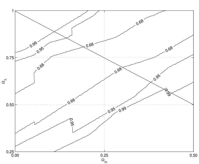
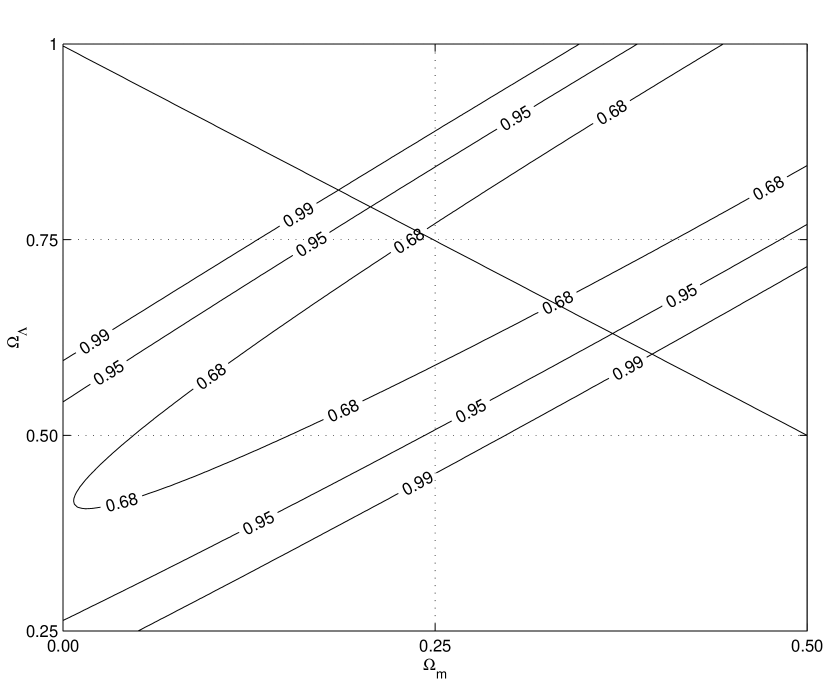
Figure 1: The $68\%$, $95\%$ and $99\%$ confidence regions resulting from standard median and $\chi^{2}$ statistics in the $\Omega_{m}-\Omega_{\Lambda}$ plane, using the 92 supernovae from the combined SCP and HzST results. A value of $H_{0}=65.2\ {\rm km\ s^{-1}\ Mpc^{-1}}$ was assumed for the Hubble parameter (see main text).

Results for the current supernova data set, using standard median and $\chi^{2}$ statistics are shown in Fig. 1 . Here we assume the knowledge of the Hubble’s constant, which we take to be $H_{0}=65.2\ {\rm km\ s^{-1}\ Mpc^{-1}}$, in agreement with Riess et al. (1998).

In a $\chi^{2}$ analysis it would be standard procedure to integrate over the Hubble parameter,

$$P(\Omega_{m},\Omega_{\Lambda})=\int P(\Omega_{m},\Omega_{\Lambda},H_{0})dH_{0},$$ (13)

but that is not the case with standard median statistics. In fact possibly the main problem with this method is its inability to cope very well with a multi-dimensional fit specially if it depends on several parameters. Clearly the Hubble parameter plays a very important part in this analysis, and a good knowledge of it is necessary to obtain good results. The factor $-5\log H_{0}$, present in the distance modulus definition as an additive constant, can move the zero-redshift point up or down the magnitude scale leaving otherwise the curve unaffected. Recall that the supernovae distance scale depends on the Large Magellanic Cloud’s distance modulus, and indeed this is the largest source of systematic error.

We note that given a sufficient number of local supernovae it is possible to calibrate the value of $H_{0}$ since when $z\ll 1$ the distance modulus is simply given by

$$\mu_{0}=5\log\frac{cz}{H_{0}}+25\,,$$ (14)

independently of the other cosmological parameters. In this way the value $H_{0}=65.2\pm 1.3\ {\rm km\ s^{-1}\ Mpc^{-1}}$ (only the statistical error is included) was found by HzST (Riess et al., 1998) which is in agreement with the HST Key Project result (Freedman, 2000).

As expected, we find a somewhat larger confidence region in the case of median statistics. Nevertheless, we can still exclude a Universe with a vanishing cosmological constant with more than $99\%$ confidence. Similarly, the confidence region is above the $q_{0}=\Omega_{m}/2-\Omega_{\Lambda}=0$ line that separates an accelerated expansion of the Universe from a decelerating one.

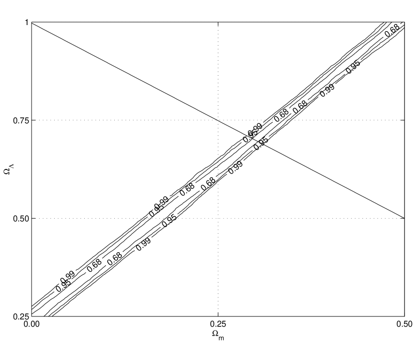
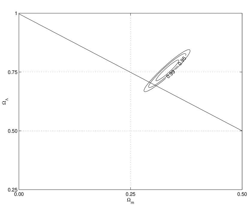
Figure 2: The $68\%$, $95\%$ and $99\%$ confidence regions resulting from standard median and $\chi^{2}$ statistics in the $\Omega_{m}-\Omega_{\Lambda}$ plane, using the SNAP-class dataset. A value of $H_{0}=65.2\ {\rm km\ s^{-1}\ Mpc^{-1}}$ was assumed for the Hubble parameter (see main text).

Fig. 2 shows an analogous analysis but now using the SNAP simulated results; again we assume the knowledge of the present day value of the Hubble parameter $H_{0}$. As expected, both statistics can now accurately pin down a ‘degeneracy axis’ but the error bars within this axis are considerably larger for median statistics.

4.2 Modified median statistics

So far we have done the analysis using the standard median statistics. We now consider the effect of the modifications which we described in the in order to take into consideration (a) the largest sequence or (b) the number of sequences obtained. We shall see that these modifications allow us to slightly improve the constraints on the parameters being estimated.

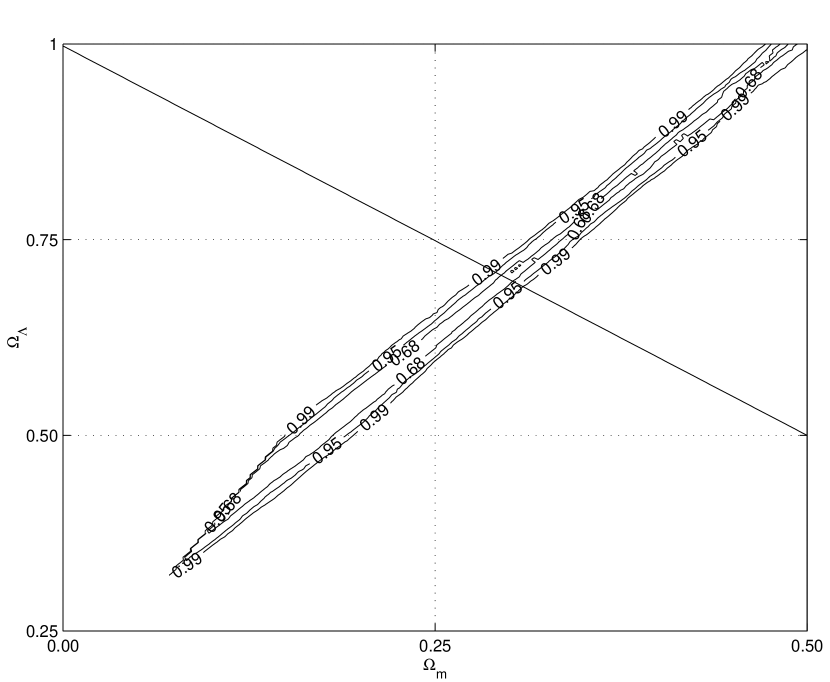
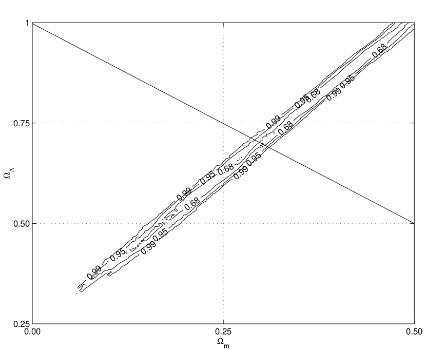
Figure 3: The $68\%$, $95\%$ and $99\%$ confidence regions resulting from modified median statistics in the $\Omega_{m}-\Omega_{\Lambda}$ plane, using the SNAP-class dataset. A value of $H_{0}=65.2\ {\rm km\ s^{-1}\ Mpc^{-1}}$ was assumed for the Hubble parameter (see main text). The first plot shows the results obtained using median statistics modified to account for the largest sequence, while in the second we consider the number of sequences.

Fig. 3 shows the results of analysing a SNAP-class mock dataset using median statistics modified to include either of the two effects (a) or (b).

We can see that either modification seems to be more constraining than standard median statistics, as it reduces the error bars within the above-mentioned ‘degeneracy axis’. This was expected, for the reasons already pointed out above: a fit where points alternate above and below a theoretical line should in principle be better than one where there are long continuous sequences either above or below it.

As one varies the present day values of the cosmological matter and vacuum densities, $\Omega_{m}$ and $\Omega_{\Lambda}$, the luminosity versus redshift curves also change. As a result of this tilting, some of these curves will mostly be above (or below) the data points at high redshift. A $\chi^{2}$ analysis will immediately disfavour these models. On the other hand, in the case of the standard median, many such models which can ‘compensate’ for this by having a fair amount of points at lower redshift below the data points will still survive. However, if one accounts for the presence of sequences and reduces the likelihood of any model where such sequences are found, then one will be able to reduce the range of allowed models. We have verified that the performance of the modified median statistics upon integration over the Hubble parameter is significantly better than that of standard median statistic but still not competitive with the $\chi^{2}$ analysis.

We also note that the gain from either of the modifications is fairly similar. Of course we could also implement them together if desired. One would obtain a further (slight) improvement, at the expense of having to deal with a somewhat more complicated statistic.

4.3 The flat case

Most inflationary models predict a flat Universe, and this seems to be confirmed by recent results from CMB anisotropy measurements (Jaffe et al., 2001). Using this prior, the precision of the fits is quite substantially increased, as we’ll be fitting for a single parameter. This can already be seen in Figs. 1–3 where the diagonal line that intersects the confidence regions represents the combinations of the cosmological parameters $\Omega_{m}$ and $\Omega_{\Lambda}$ which correspond to a flat universe.

In the case of a flat universe the modifications we made to median statistics do not significantly improve the constraints on $\Omega_{m}-\Omega_{\Lambda}$ plane obtained using the conventional median analysis and so we’ll restrict ourselves to the standard case.

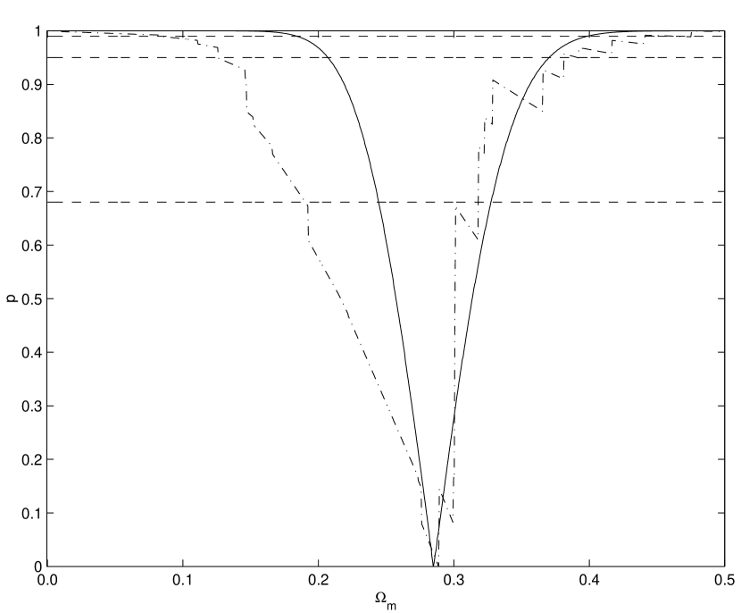
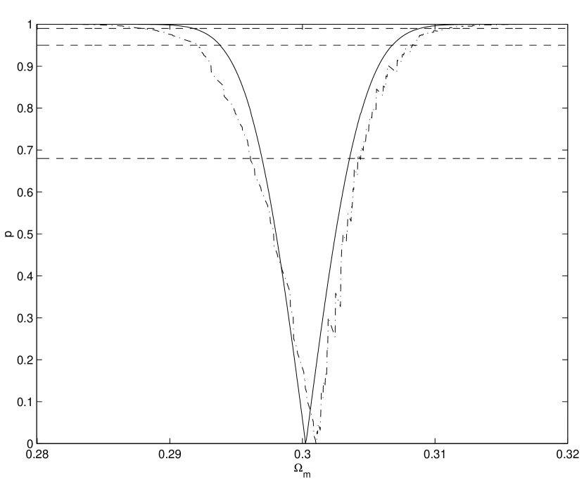
Figure 4: Marginal distributions for $\Omega_{m}$ obtained using the standard median (dot-dashed) and $\chi^{2}$ (solid line) statistics, assuming a flat Universe, for the current and the SNAP-class datasets. The $68\%$, $95\%$ and $99\%$ confidence limits are where the curves drop below the (dashed) lines of constant $p$ (0.68,0.95 and 0.99 respectively). Note that a value of $H_{0}=65.2\ {\rm km\ s^{-1}\ Mpc^{-1}}$ was assumed for the Hubble parameter.

In Fig. 4 we show results obtained for both datasets through the methods previously presented, assuming a flat universe prior using the conventional median statistic and the $\chi^{2}$ statistic. We present these results in a more convenient form in table 2.

For a flat Universe we obtain $\Omega_{m}=0.29^{+0.03}_{-0.10}$ (not including the uncertainty in the Hubble parameter) using currently available supernovae and simple median statistics. For these 92 supernovae the median statistic is marginally less competitive than the $\chi^{2}$ statistic and one notices that the median results are slightly skewed towards low values of $\Omega_{m}$. Nevertheless the $90\%$ confidence upper limit for $\Omega_{m}$ is slightly lower in the case of median statistics and the confidence intervals still overlap nicely.

Clearly the SNAP results are expected to significantly improve the constraints on the energy density of the Universe. Note that the results obtained with median statistics are almost indistinguishable from those obtained with the standard $\chi^{2}$ analysis in this case.

This analysis clearly show that the median and the standard $\chi^{2}$ statistics have quite similar performances if the assumptions about a Gaussian distribution for the errors and the estimate of the standard deviations are correct. If this is not the case, then obviously the results obtained with the median statistic are the more reliable ones.

Indeed, one could use this information to reverse the argument and use both statistics together as a test on the assumptions being made on the data. If in the case of SNAP the median and $\chi^{2}$ statistics do not agree, then this indicate that either the errors do not have a Gaussian distribution or that one is somehow underestimating the statistical and/or systematic errors.

Table 2: Values of $\Omega_{m}$ obtained through median statistics for supernova data (both the current and the SNAP datasets) with a flat universe prior. Results for the usual $\chi^{2}$ statistic are also shown for comparison. Here a value of $H_{0}=65.2\ {\rm km\ s^{-1}\ Mpc^{-1}}$ was assumed for the Hubble parameter

Statistic	Current data set	SNAP data set
Median	$0.29^{+0.03}_{-0.10}$	$0.301^{+0.004}_{-0.005}$
Chi Squared	$0.28^{+0.05}_{-0.04}$	$0.300^{+0.004}_{-0.003}$

5 Conclusions

We have discussed standard and modified median statistics in the context of current and forthcoming type Ia supernova data sets. The purpose of the modifications is to reduce some of its weaknesses, mainly by accounting for the number and size of sequences of consecutive points above or below the median. We found that in some circumstances the performances of the median and $\chi^{2}$ statistics can be comparable, and if used together they provide a simple test on the assumptions being made on the data.

The main problem with the standard median statistics analysis is its inability to cope well with a multi-dimensional fit specially if it is dependent on several parameters. This is due to the very simple assumptions it makes. On the other hand, when confronted with a single parameter to fit, the ensuing results can be of similar precision to the ones obtained with a $\chi^{2}$ analysis.

Another advantage of median statistics is that it is an analysis method which is extremely easy to implement. So even in the cases where it is not expected to produce results as constraining as a $\chi^{2}$ analysis, it can be used to complement it or to provide fast fits in the early stages of the analysis, notably if one is still trying to gather supporting evidence for the use of stronger hypothesis about the dataset. Using median statistics we no longer have to suppose that the errors follow a Gaussian distribution with known standard deviation, and can therefore have greater confidence in the parameter ranges obtained. This is an important concern for the particular case of type Ia supernovae: recall that when studying them we are considering renormalised light curves, and that the calibration data set (of nearby supernovae) is smaller than the main data set (of distant supernovae). The median statistic is also less sensitive to systematic effects such as weak lensing.

We have studied some simple means by which to improve median statistics, namely accounting for the size of the largest sequence or the number of sequences present in the dataset above or below the model prediction, Our adjustments did provide some improvement, even if in a our confidence regions are still larger than that obtained from a $\chi^{2}$ study. We note however that other more ‘baroque’ modifications are certainly conceivable. Other possibilities, which certainly deserve further work, are to study how similar procedures could be used to improve the standard $\chi^{2}$ analysis (which is sequence blind), and to apply median statistics to other cosmological data sets, most notably the cosmic microwave background. We shall report on these issues in a forthcoming publication.

References

- Bean & Melchiorri (2002) Bean, R. & Melchiorri, A. 2002, Phys. Rev. D65, 041302
- Bucher (1999) Bucher, M. 1999, Phys. Rev. D60, 043505
- Caldwell, Dave, & Steinhardt (1998) Caldwell, R. R., Dave, R. & Steinhardt, P.1998, Phys. Rev. Lett.80, 1582
- Carroll, Press & Turner (1992) Carroll, S., Press, W. & Turner, E.L. 1992, Ann. Rev. Astron. Astrophys. 30, 499
- Freedman (2000) Freedman, W. L. 2000, Phys. Reports 333, 13
- Gott et al. (2001) Gott, J. R. et al. 2001, ApJ549, 1
- Jaffe et al. (2001) Jaffe, A. H. et al. 2001, Phys. Rev. Lett.86, 3475
- Nugent (2000) Nugent, P. 2000, SNAP: Supernova acceleration probe: An experiment to measure the properties of the accelerating universe. See homepage at http://snap.lbl.gov
- Peebles & Ratra (1988) Peebles, P.J.E. & Ratra, B. 1988, ApJ325, L17
- Perlmutter et al. (1999) Perlmutter, S. et al. 1999, ApJ517, 565
- Phillips et al. (1999) Phillips, M. M. et al. 1999, AJ118, 1766
- Podariu & Ratra (2000) Podariu, S. & Ratra, B. 2000, ApJ532, 109
- Ratra & Peebles (1988) Ratra, B. & Peebles, P.J.E. 1988, Phys. Rev. D37, 3406
- Riess et al. (1998) Riess, A. et al. 1998, AJ116, 1009
- Waga & Frieman (2000) Waga, I. & Frieman, J. 2000, Phys. Rev. D62, 043501
- Wang et al. (2000) Wang, L. et al. 2000, ApJ530, 17
- Wang et al. (2000) Wang, Y. et al. 2000, ApJ536, 531
- Weller & Albrecht (2001) Weller, J., and Albrecht, A. 2001, astro-ph/0106079