Galaxy colours in high redshift X-ray selected clusters – I: Blue galaxy fractions in eight clusters

Abstract

We present initial results from a wide–field, multi–colour imaging project, designed to study galaxy evolution in X-ray selected clusters at intermediate ($z\sim 0.25$) and high redshifts ($z\sim 0.5$). In this paper we give blue galaxy fractions from eight X-ray selected clusters, drawn from a combined sample of three X-ray surveys. We find that all the clusters exhibit excess blue galaxy populations over the numbers observed in local systems, though a large scatter is present in the results. We find no significant correlation of blue fraction with redshift at z$>$0.2 although the large scatter could mask a positive trend. We also find no systematic trend of blue fraction with X-ray luminosity. We show that the blue fraction is a function of (a) radius within a cluster, (b) absolute magnitude and (c) the passbands used to measure the colour. We find that our blue fractions ($\rm f_{b}$) from galaxy colours close to restframe $(U-B)_{0}$, $\rm f_{b}\,\sim\,0.4$, are systematically higher than those from restframe $(B-V)_{0}$ colours, $\rm f_{b}\,\sim\,0.2$. We conclude this effect is real, may offer a partial explanation of the widely differing levels of blue fraction found in previous studies and may have implications for biases in optical samples selected in different bands.

While the increasing blue fraction with radius can be interpreted as evidence of cluster infall of field galaxies, the exact physical processes which these galaxies undergo is unclear. We estimate that, in the cores of the more massive clusters, galaxies should be experiencing ram–pressure stripping of galactic gas by the intra–cluster medium. The fact that our low X-ray luminosity systems show a similar blue fraction as the high luminosity systems, as well as a significant blue fraction gradient with radius, implies other physical effects are also important.

1 Introduction

During the past few decades, numerous studies of the optical properties of galaxy populations within clusters have allowed an intriguing insight into the processes that govern the evolution of galaxies. Rich galaxy clusters provide a large sample of galaxies, at a similar redshift and of various masses and morphological type with which to probe these phenomena. One of the most influential early results, which motivated many successive studies was that of ?. In this study of two high redshift clusters they found a large fraction of galaxies in the inner regions of the cluster with colours significantly bluer than the colour–magnitude relation (CMR) of the cluster ellipticals (Es). ? extended this study to include 33 clusters and found an increasing trend in this blue fraction ($f_{B}$) with redshift, above $z\sim 0.1$. A number of subsequent photometric studies have generally confirmed the presence of these excess blue galaxies, though in varying quantities (e.g. ?; ?; ?; ?). Subsequently spectroscopic investigations not only confirmed the cluster membership of large numbers of these galaxies but also discovered that their spectra contained features indicative of star formation, often recently truncated (?; ?; ?; ?).

During these studies it became increasingly clear that whilst the luminous elliptical galaxies present in cluster cores have undergone little but passive evolution since higher redshift ($z\geq 1$, e.g. ?; ?), a major change has taken place in the other morphological types. Specifically the large S0 population found in local clusters are found to be almost absent in high redshift ($z\sim 0.5$) clusters (?), where evidence pointed towards the excess blue galaxies often having spiral morphologies. Confirmation of this came with morphological studies using $HST$. ? and ? found that not only were the blue galaxy populations disk dominated, but they often exhibited signs of interaction. It is now generally thought that these photometric, spectroscopic and morphological evolutionary effects are related. The suggestion being that at higher redshifts, bluer field galaxies, generally spirals, that are drawn into the core regions of clusters have their star formation quenched by some mechanism. They then proceed to evolve morphologies, possibly by some form of mass loss, into the large S0 population seen in the core of rich clusters today. Perhaps the most surprising aspect of these phenomena, though, is the rapid rate at which this evolution takes place.

Clearly understanding the processes behind this evolution is vital to our understanding of how galaxy histories have progressed. Whilst observational data is becoming ever more available, the mechanisms causing this evolution are less well understood. Several suggestions have been put forward to explain the effects of the interaction of galaxies with their environment and each other. Certainly in the cores of clusters, where the intra–cluster medium (ICM) is densest, infalling galaxies, with smaller gravitational potential wells, will suffer from ram–pressure stripping of their gas (e.g. ?; ?). Other mechanisms which may affect smaller galaxies include tidal effects generated by the cluster potential (?) or galaxy harassment caused by close encounters with other galaxies (?; ?). In addition to these processes the direct interaction and merging of galaxies is also a possibility, especially in poorer clusters, with shallower gravitational potential wells (e.g. ?).

Most studies till now have looked at massive clusters, nearly all of which have been optically selected. Several large photometric surveys, for instance, have used optically selected, such as ?, clusters (e.g. ?; ?; ?). Differing blue fractions, however, were found in these investigations, with ? claiming a blue fraction of up to 80 percent in high redshift clusters. Investigations based on clusters selected in other wavebands have only recently been undertaken. ? conducted a photometric study of galaxies around bright radio–galaxies up to $z\,\sim\,0.45$, and found evidence for enhanced blue populations in most systems at higher redshift. The galaxy systems observed contained a number of poorer clusters and no relationship between blue galaxy fraction and redshift was found. They concluded that the increase in blue fraction in high redshift, rich clusters was due to processes inefficient in poorer systems.

The other area which has only recently begun to be explored is the selection of clusters, for optical study, via the X-ray emission from their intra–cluster medium (ICM). ? used a sample of 10 intermediate redshift ($z\,\sim\,0.25$), high X-ray luminosity, X-ray selected clusters in a multi–colour study of their galaxy populations. They found low blue fractions, with the bluer galaxies tending to avoid the cluster cores. The other main exploration of optical galaxy properties within X-ray selected clusters is that of the Canadian Network for Observational Cosmology (CNOC, ?). They find excess blue galaxies in distant clusters (e.g. ?), colour, emission line, population and age gradients within the clusters (?, ?), and a fraction of luminous “K+A” cluster galaxies (with strong Balmer absorption lines but no emission lines) which is similar to that in the field at z$\approx$0.3 (?). The combined N-body and semi-analytic models of ? match the CNOC1 cluster observations and support a gradual termination of star formation after cluster infall. ?, using 7 clusters drawn from the CNOC sample also find an excess of blue galaxies.

Whilst a general consensus as to the presence of this excess star–formation is evident, the level of it, and the evolutionary nature is less clear, with a major question being the steepness of the increase of blue galaxy population with redshift (e.g. ?). Blue fraction may, or may not, be a function of redshift and X-ray luminosity, which may cause significant biases in studies limited to a small sample of clusters, within a limited range of redshifts or samples compiled for comparison which have varying X-ray luminosities (e.g. ?). The works of ?, ? and ? hint at there being no clear relation between blue fraction and X-ray luminosity. Additionally, the changing environmental nature of the clusters may also have a large effect, for instance excess sub–structure may bias towards higher blue fractions (?). It can, therefore, be seen that the large spread in observed results highlights the need for a method of cluster selection which avoids the biases inherent in optical selection, whilst still providing large catalogues of galaxy clusters with multifarious properties to allow exploration of the redshift, cluster properties and environment parameter space.

This paper, the first in a series, presents details of analysis and initial results from multi–colour, wide–field imaging of an X-ray selected sample of galaxy clusters. The clusters span a large range in X-ray luminosity (a factor of 100 in the 8 clusters presented here) whilst being constrained to two redshift bands designed to minimise the effects of k–correction. This project, on completion, should allow an insight into the evolution of galaxies within a variety of cluster environments, selected solely according to their X-ray properties. The organisation of the paper is as follows. In the next section we discuss further the subject of the selection of the sample of clusters presented here. We then detail the observations used in this paper, before discussing the reduction and analysis techniques used. We then present and discuss results from the photometry, including colour–magnitude diagrams and blue fractions. Our conclusions are drawn in the final section. In order to allow comparison to other works we consider an $\rm H_{0}=50\>km\>s^{-1}\>Mpc^{-1}$ and $\rm q_{0}=0.1$ cosmology throughout this paper.

2 Sample selection

Cluster	Redshift	$\rm L_{x}(\rm erg\,s^{-1})$	Filters	Exposure (ks)	Completeness
RXJ1633.6+5714	0.239	$0.12\times 10^{44}$	$B,V,R$	3.00, 1.20, 1.20	24.3, 24.2, 23.5
MS1455.0+2232	0.259	$11.51\times 10^{44}$	$B,V,R$	2.24, 2.40, 2.70	24.0, 23.9, 22.5
RXJ1418.5+2510	0.294	$3.66\times 10^{44}$	$B,V,R$	3.60, 1.20, 1.20	24.2, 23.9, 22.4
RXJ1606.7+2329	0.310	$0.85\times 10^{44}$	$B,V,R$	3.60, 1.20, 1.20	24.2, 24.1, 22.5
MS1621.5+2640	0.426	$4.71\times 10^{44}$	$V,R,I$	8.40, 5.40, 1.80	24.0, 23.9, 22.9
RXJ2106.8-0510	0.449	$2.79\times 10^{44}$	$V,R,I$	6.90, 4.20, 1.80	24.2, 24.1, 22.9
RXJ2146.0+0423	0.532	$4.27\times 10^{44}$	$V,R,I$	6.00, 2.40, 1.80	24.4, 24.2, 22.8
MS2053.7-0449	0.583	$5.49\times 10^{44}$	$V,R,I$	6.00, 3.90, 1.80	24.0, 23.8, 22.8

Table 1: Details of the 8 X-ray selected clusters. Redshifts are spectroscopically confirmed. X-ray luminosities from the $ROSAT$ PSPC are given in the 0.5–2 keV band. Listed are the filters used, along with the respective exposure times. Finally apparent magnitude completeness limits are given, estimated from N(m) plots.

As discussed in the previous section, the need for an unbiased cluster sample with which to investigate galaxy evolution is of paramount importance. This is certainly the case when trying to construct a picture of the various mechanisms that affect the changing morphologies and star formation histories of cluster galaxies. Whilst the studies of optically rich clusters have given evidence for rapid evolution in galaxy colours, this is by no means a universal result. Indeed even within the ? analysis, the scatter on the blue fraction versus redshift plot is large. For instance CL0016+16, A2397 and A2645 (at redshifts 0.541, 0.224 and 0.246 respectively), to name but a few, all demonstrate little, if any, evidence for enhanced blue fraction. This may be indicative of the fact that optically selected high redshift clusters, which traditionally were often selected in a blue rest frame (e.g. ?; ?), may be an unrepresentative sample and biased towards high blue fractions. Indeed ?, using an X-ray selected sample of X-ray luminous massive clusters found evidence of a spread in blue fractions, though with a low median value ($\rm f_{b}=0.04$ for concentrated clusters, for which ? found $\rm f_{b}=0.09$ for a similar sample), and hence generally low star formation rates. The goal of this project, therefore, is to construct a sample of galaxy clusters where the selection of the clusters is independent of the galaxy properties, with which to investigate cluster galaxy evolution. Additionally we wish to explore a wide range of cluster masses (as indicated by their X-ray luminosities) and be able to make comparisons between similar mass clusters at different redshifts.

The clusters used in this study are drawn from the catalogues of three major cluster surveys. The $Einstein$ Medium Sensitivity Survey (EMSS, ?) has a higher flux limit than the two other surveys used and thus primarily contributes brighter X-ray clusters. In addition we use two other serendipitous cluster catalogues based on archival, $ROSAT$ PSPC data. These are the Southern–Serendipitous High–redshift Archival $ROSAT$ Cluster survey (S–SHARC, ?; ?) and the Wide Angle $ROSAT$ Pointed Survey (WARPS, ?; ?). All of these surveys use the X-ray emission from diffuse gas, trapped in the gravitational potential well of a cluster, as tracers for the mass of the cluster. Optical imaging and spectroscopic follow–up then confirms the presence and redshift of the clusters from a few of their brightest galaxies. This method has the considerable advantage over optical surveys of nearly eliminating biasing caused by projection effects and erroneous identifications (?; ?; ?). Whilst the three X-ray surveys used as a basis for this study vary in their flux limits and detection techniques, they are all based on the detection of an X-ray flux in a similar energy range, and they all corrected from measured luminosities to total luminosities in a similar manner, assuming a King surface brightness profile. Mean differences in total flux estimates between X-ray surveys are typically $\approx$20 percent (e.g. ?, ?).

We attempted to restrain the redshift ranges of our cluster sample to minimise the effects of k-correction between bands. To this end we selected two redshift bands for our clusters, in which redshift corrected standard Johnson–Kron–Cousins filters ($BVR$ in the low redshift sample, $VRI$ in the high) were mapped onto rest frame $UBV$ filters, as much as possible. The limited number of X-ray selected clusters in any given RA range, however, prevents a very tight constraint in redshift range. For the purposes of this initial study, eight clusters were included in our sample for observation. These were chosen to maximise the spread in X-ray luminosity within the constraints placed by the RA range of this first observing run. Details of these clusters can be found in Table 1. Here we give cluster IDs along with spectroscopically confirmed cluster redshifts. All the clusters in this sample have a reasonably relaxed X-ray morphology as detected in their $ROSAT$ PSPC data. They should, thus, be good examples of reasonably relaxed systems. The blue fraction of one of our sample, MS1621.5, has been studied previously (?; ?) and thus will allow comparison to this investigation, providing a good consistency check. The sample presented here is by no means complete. Future papers will detail observations expanding the sample to fill out the redshift and X-ray luminosity parameter space.

3 Observations

The eight clusters detailed in Table 1 were observed on June 17–20th 1999 using the Wide Field Camera (WFC, ?) on the 2.5 metre Isaac Newton Telescope (INT) on La Palma. The WFC consists of 4 thinned EEV CCDs each having 0.33 arcsec/pixel resolution and giving a combined spatial coverage of $\rm\sim 0.29\,deg^{2}$ (each 22.8 by 11.4 arcmin) at telescope prime focus. The 4 CCDs exhibit varying characteristics with, in particular, the gain of the central CCD being lower than the others. In addition there is some non-linearity apparent in all CCDs, with the most non-linear varying by around 6 percent over the entire dynamic range. The large sky coverage of the WFC allows us, generally, to image the entirety of the target cluster in the central CCD. In the cosmology used in this paper, $\rm H_{0}=50\>km\>s^{-1}\>Mpc^{-1}$ and $\rm q_{0}=0.1$, the 5.7 arcmin half width of our central CCD corresponds to a little over 1.7 Mpc, for our nearest cluster, and around 2.9 Mpc for our most distant. In addition the WFC also provides a highly accurate statistical estimation of the local background of the cluster, without the need for separate calibration fields. This will hopefully reduce the affect of large–scale structural variations on our investigation. We observed each of the eight clusters in three filters, $BVR$ and $VRI$ for the low and high redshift clusters respectively. Details of the exposure times obtained are given in Table 1. In each case we aimed to achieve good signal–to–noise down to at least $\rm M^{*}\,+\,3$ ($\rm M_{V}\approx-19$). In addition we give the cluster X-ray luminosity from the $ROSAT$ PSPC (0.5–2 keV). Most observations were carried out near zenith and seeing conditions were found to be generally good, ranging from 1.52 to 0.79 arcsec FWHM.

4 Data reduction and Analysis

4.1 Reduction and calibration

Initial reduction was carried out in the standard way. After bias subtraction and non-linearity corrections (obtained from the Wide Field Survey (WFS, ?)) were applied, the images were flat–fielded. Large scale gradients were observed in the $B$, $V$ and $R$ filters after application of twilight flats, so instead it was decided to use data flats median combined from the dithered science images, with masks designed to eliminate bright galaxies and stars. Due, however, to the low number of target clusters observed during each night, allied to lengthy exposures (chosen because of long readout times), the number of images available for median combination each night was insufficient to generate statistically acceptable flat–fields. It was therefore necessary to combine data from more than one night. We used median combined data flats combined from two nights, in the $V$ and $R$ bands. In the case of the $B$ band exposures, data was taken on only three nights, and all were required to provide an adequate flat. In the cases of the $I$ and $R$ band exposures, night sky fringing was apparent. In the $R$ band this was found to be virtually eliminated by flat–fielding using data flats. The level of fringing in the $I$ band, however, was significantly higher (of the order of three percent deviation from sky level). The reduction of the I band thus followed a slightly different pattern. Here we used the twilight flat–field which produced highly fringed, though generally flat images. We proceeded to produce a master fringe frame from all of our $I$ band data and this was used to de–fringe our data. We used an iterative process to scale the master fringe frame to the approximate level of the fringes; subtracting this left a residual fringe level in each image, which could be used to adjust the subsequent level of the scaling. After final de–fringing, our images typically showed residual fringing at $\stackrel{{\scriptstyle<}}{{{}_{\sim}}}\,0.3$ percent of sky level. The above steps were carried out independently on each CCD. Figure 1 contains an example $V$ band image of the central region of RXJ1418.5. Overlayed upon this image are X-ray contours from the $ROSAT$ PSPC.

At least twelve sets of ? standard star fields (Landolt 107,110,113) were observed in various filters, each night, to allow accurate photometric zero–points to be obtained for each CCD. Our first night was found to be non–photometric, though in all cases clusters observed during this night had short exposure calibration images taken on one of the following nights. Nights 3 and 4 of the observations appeared to be totally photometric and the atmospheric absorption on these nights was found to be consistent with the standard values of the La Palma site, and thus we adopted these. It was found that an excess amount of atmospheric absorption was present on the second night ($R\approx 0.30$ mag at zenith). This appeared to be present and contributing similar absorption in all bands and did not appear to vary throughout the night. We attribute this roughly grey absorption to atmospheric dust. It was also observed (with a slightly larger magnitude ($r^{\prime}\approx 0.38$)) in the $r^{\prime}$ band standard star measurements at the Carlsberg Meridian telescope, on La Palma, during the same period. Zero points and colour equations were devised for each CCD, in each filter on each night, in order to place the photometry on the standard Johnson–Kron–Cousins system. Although the final solutions to these equations had rms deviations of less than 0.005 mag, the maximum final absolute photometric error, including systematic effects, was estimated to be $\stackrel{{\scriptstyle<}}{{{}_{\sim}}}\,0.03$ mag. This estimation was based on standard star deviations from our best fit solutions, as well as from external checks which are discussed in the next section. In general the solutions were consistent with those obtained by the Wide Field Survey. In addition zero–points were adjusted for the affects of galactic absorption, for each cluster pointing, using absorption maps from the $IRAS$ satellite (?).

4.2 Constructing photometric catalogues

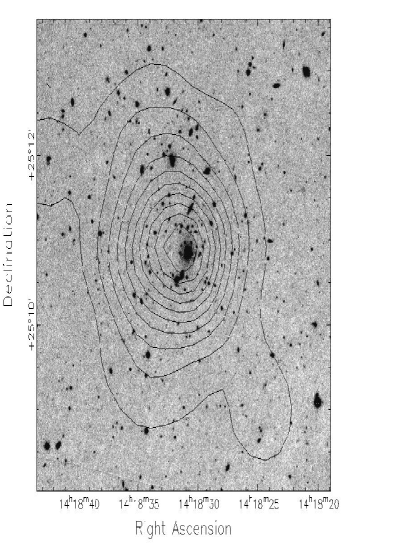
Figure 1: INT WFC $V$ band image of RXJ1418.5+2510 at $z=0.294$. Overlayed on the image are contours of the X-ray emission detected from this $\rm L_{x}\,=\,3.66\,\times\,10^{44}\,erg\,s^{-1}$ (0.5-2 keV) cluster from the $ROSAT$ PSPC. Contours are equally spaced in flux level and were derived from an image smoothed to PSPC resolution. Only a small fraction ($\sim 2$ percent) of the total WFC image is shown.

Figure 2: A composite number–magnitude diagram for the combined backgrounds of the clusters in the $R$ band. Different symbols represent the 8 different clusters. Error bars are included but are generally smaller than the point size. The lines overlayed are from the works of Jones et al. (1991); Metcalfe et al. (1991, 1995); Steidel & Hamilton (1993) and Smail et al. (1995). The turnover due to incompleteness generally occurs at brighter magnitudes for the lower redshift clusters.

Galaxy photometry catalogues were constructed using the SExtractor package (?). This allows detection of objects in one image, with additional photometric analysis from another. Our images were aligned and trimmed to provide the same sky coverage for all filters for each CCD. Detection was carried out in the reddest filter image for each cluster (i.e. $I$ band for the higher redshift clusters, $R$ band for the lower) so as not to exclude the redder cluster galaxies. Detection significances of more than $1.5\,\sigma$ per pixel were required consisting of at least 9 contiguous pixels. We used the observed colour of each galaxy, with the appropriate colour equation, to give accurate magnitudes. We used matching aperture magnitudes for colour estimation, with the aperture size, a 6 pixel radius equivalent to 2.0 arcsec, larger than the worst seeing in any of our images. Kron–type magnitudes were measured, using the default SExtractor settings, to provide the best estimate of the total magnitudes of the galaxies.

After elimination of objects with unreliable photometry due to, for instance, proximity to CCD edge, star/galaxy separation was achieved using the SExtractor CLASS_STAR parameter estimated from the two reddest bands for each cluster. At fainter magnitudes all star/galaxy classification begins to fail, thus we limited our separation to brighter than an apparent magnitude of $I=22$, $R=22.5$ and $V=23$. A number of fainter stars will thus be retained, however at these fainter magnitudes galaxy counts dominate (e.g. ?) and the stars will remain in both cluster and field images and so should be naturally accounted for. In the case of SExtractor detection in our $I$ band images, a few false detections were noticed by visual inspection, these coincided with residual fringes in the images. The photometry extracted from the other two filters, however, showed no sign of these detections and so provided a useful robustness check. All galaxies not detected in at least two of the bands were excluded from our analysis. This cut may also exclude objects of extreme colour towards our magnitude limit, these however generally fall well below the magnitude cuts used in the analysis presented here.

Number–magnitude plots of galaxies were generated allowing us to make conservative estimates of the apparent magnitude completeness level of each observation. An example of one of these plots is shown in Figure 2. Here we plot the number-magnitude relations for the $R$ band observations of the combined background fields of all our clusters, in 0.5 magnitude bins. Overlayed on this plot are best fit lines from previous large scale galaxy number counts investigations (?; Metcalfe at al. 1991, 1995; ?; ?). It can be seen that, whilst all of our backgrounds are in reasonable agreement with the previous studies, a significant spread in normalisation is found (up to a factor of around 1.5 difference). This is important as it emphasizes the advantage of having large background areas surrounding the cluster, which can then be used to take account of variations in the field galaxy density used for the statistical analysis. Completeness levels estimated from the number–magnitude plots are also given in Table 1. The variations between exposure times and completeness levels are due to the varying observational conditions. In most cases the completeness levels correspond to reaching our original target depth of $\rm M_{V}\,=\,-19$ (one magnitude deeper than that used in ?) in our cosmology. We miss $\rm M_{V}\,=\,-19$ by about 0.5 magnitudes for our most distant cluster, MS2053.7-0449. In addition to the calibration provided by our standard star measurements we use two other independent diagnostics to confirm our photometry. The field of RXJ1418.5+2510 has Johnson $B$–band magnitudes of several stellar sources published by ?, which agreed to $B$ $>$ 21.5 with our measured magnitudes, to within 0.03 mag rms. The other checks are of a more statistical nature. We generated galaxy and stellar count and colour histograms for several of the background fields of our clusters. These were then compared to those published by ? and again gave good agreement, given statistical fluctuations. For instance our average ${(B-R)}_{CCD}$ colours of field galaxies (when converted to the filter colours of ?) for our four low redshift cluster fields were 1.79, 1.75 and 1.79 (in the magnitude ranges $19.5\!<\!R_{CCD}\!<\!20$, $20\!<\!R_{CCD}\!<\!20.5$ and $20.5\!<\!R_{CCD}\!<\!21$ respectively) which compare well with the corresponding values of 1.70, 1.93 and 1.78 (from ?), given the sizeable statistical errors and large scale structure variations.

4.3 Galaxy density profiles

The variation in cluster mass built into our sample means that each cluster has a different physical size. This is important to take into consideration when comparing the populations of the various clusters. Matched physical sizes will not provide an accurate comparison, as clusters cores are known to contain galaxy populations with different characteristics to those in more outlying regions (e.g. ?; ?). A better analysis technique would be to use the galaxy population as an indicator of the cluster size.

? detail a method of estimating matched radial distances in clusters from their galaxy density profiles. They define a concentration parameter

$$\rm C=log(R_{60}/R_{20})$$ (1)

where $\rm R_{n}$ represents the radius containing n percent of the total cluster population. For each of our clusters, radial galaxy density profiles were generated, allowing estimates of the cluster concentration parameter and the radius of the cluster which contained 30 percent of the cluster galaxies ($\rm R_{30}$, as used for blue fraction calculations in ?).

It was clear from the statistically background subtracted radial profiles where the cluster over-density reached the background levels, and this allowed estimates of the characteristic radii from the integrated population within this boundary. The large background fields available for each cluster served to reduce the error in the background level estimates. The derived values of $\rm R_{30}$ were not sensitive to the details of this procedure, and for all our clusters $\rm R_{30}$ lay well within the cluster CCD. Our $\rm R_{30}$ and concentration parameter values for each cluster are detailed in Table 2. It is reassuring to note that all our clusters have concentration parameters above 0.4, which would be expected from the relaxed nature of their X-ray contours. It is these concentrated clusters which were used by ? to fit a trend line which defined the Butcher-Oemler effect.

4.4 Bright galaxy area correction

The main complication of generating accurate radial profiles is the estimation of the number of fainter galaxies lost behind brighter and larger galaxies in the foreground. To solve this problem we calculated the total area lost behind brighter galaxies, in each radial bin used for this calculation. We chose all galaxies above 300 pixels in size and estimated the area they occupied, within the radial bin area, at a brightness level above their detection threshold where blended galaxies would not have been detected. The area used in the calculations was then corrected for this lost area. On average the correction was of order one percent for the field frames and around two percent for the cluster fields, which agrees well with previous analyses (e.g. ?).

5 Results

5.1 Colour–magnitude diagrams

Figure 3: Colour–magnitude diagrams for five X-ray selected clusters. Here we plot the colours which correspond approximately to $(B-V)_{0}$ versus $V_{0}$ at rest: observed $V-R$ against $R$ for MS1455.0+2232 ($z=0.259$, $\rm L_{x}=11.51\times 10^{44}\,erg\,s^{-1}$), RXJ1633.6+5714 ($z=0.239$, $\rm L_{x}=0.12\times 10^{44}\,erg\,s^{-1}$) and RXJ1606.7+2329 ($z=0.310$, $\rm L_{x}=0.854\times 10^{44}$), and $R-I$ against $I$ for RXJ2106.8-0510 ($z=0.449$, $\rm L_{x}=2.9\times 10^{44}\,erg\,s^{-1}$) and MS2053.7-0449 ($z=0.583$, $\rm L_{x}=5.5\times 10^{44}\,erg\,s^{-1}$). Also shown is a composite plot of the CM diagrams of the background fields of RXJ1606. Only galaxies within $\rm R_{30}$ are shown. Our best fitting CMRs are shown as the solid lines. Blue galaxy cuts used in determining the blue fraction are shown as the dashed lines below the CMR line. Vertical dot–dashed lines represent a rest frame $\rm M_{V}\!=\!-20$ magnitude cut, whilst the triple dotted–dashed line diverging from this illustrates the effect of the different level of k-corrections for varying galaxy colours. The small boxes at the bottom of each CM diagram represent average colour and magnitude photometry error boxes, at the corresponding magnitudes. Finally the plots have sloped dotted lines which illustrates if and where our 100 percent completeness level impinges upon the CM diagram.

Figure 4: Colour–magnitude diagrams for the three remaining X-ray selected clusters. Here we plot the colours which correspond approximately to $(U-B)_{0}$ versus $V_{0}$ at rest: observed $V-R$ against $I$ for MS1621.5+2640 ($z=0.426$, $\rm L_{x}=4.71\times 10^{44}\,erg\,s^{-1}$) and RXJ2146.0+0423 ($z=0.532$, $\rm L_{x}=4.27\times 10^{44}\,erg\,s^{-1}$), and $B-V$ against $R$ for RXJ1418.5+2510 ($z\,=\,0.294$, $\rm L_{x}=3.66\times 10^{44}\,erg\,s^{-1}$). Also shown is a composite plot of the CM diagrams of the background fields surrounding MS1621.5. Again in all these cases galaxies within $\rm R_{30}$ are shown. The lines drawn on the plots represent the same as in the previous figure.

Cluster plus field colour–magnitude (CM) diagrams were generated, along with field CM diagrams from the three non–cluster CCDs. This allowed a statistical background subtraction to be carried out, for the purposes of illustration of cluster against field galaxies. This was achieved by assigning a membership probability to each galaxy, determined from the expected number of galaxies from the background fields. We then used a Monte–Carlo technique, analogous to that used in ?, to assign probabilities of cluster membership to each galaxy. The large background area meant that this could be achieved in small boxes of size 0.1 mag in colour and 0.5 mag in apparent magnitude.

In Figure 3 we present five statistically background subtracted CM diagrams, in which we show colours corresponding approximately to restframe $B-V$ versus $V$. We plot the apparent $R$ magnitude against ($V-R$) colour for MS1455.0, an X-ray luminous cluster and similarly we show ($V-R$) against $R$ for RXJ1633.6 and for RXJ1606.7, two of our low $\rm L_{x}$ clusters. We also plot apparent $I$ magnitude against ($R-I$) colour for RXJ2106.8 and MS2053.7, two high redshift clusters. Crosses represent galaxies statistically flagged as cluster members and dots represent the statistical field population. Additionally the corresponding composite field CM plot for the background fields of RXJ1606.7 is also plotted.

In Figure 4 we show CM plots of the three remaining clusters. Here though we plot colours corresponding approximately to restframe $U-B$ versus $V$. Additionally the corresponding composite field CM plot for the background fields of MS1621.5 is shown opposite it. At the bottom of each of these plots are boxes representing an average error on our photometry. The errors on the colours were taken from the error on the aperture photometry and added in quadrature. As can be easily seen, only in our faintest galaxies does the error on our colours begin to reach a level where it would effect our results.

Also shown in Figure 3 are our completeness limits, if they impinge upon the CM graph. In these cases, only RXJ2106.8 is affected. The sloped, dotted line in the top–right hand corner represents our conservative estimate of the 100 percent completeness level. We do not expect this limit to seriously effect our blue fraction results, at the magnitude levels of $\rm\sim\,M_{V}=-20$. Additional evidence for this comes from the corresponding CM diagram of MS1621.5, from ?, which does not show any excess red population near our completeness limit. In the cases of the graphs displayed in Figure 4, the completeness limit is harder to display, as it is a function of all three filter magnitudes. We make an attempt to constrain these by using colour–colour plots of our galaxies, which will be presented in more detail in a forthcoming paper. We find that for our low redshift sample we are 100 percent complete in $B-V$ at $\rm M_{V}=-20$, and estimate that this drops to around 95 percent completeness at $\rm M_{V}=-19$. For our higher redshift sample the results are poorer. Only in MS1621.5 are we fully complete to $\rm M_{V}=-19$ . In the cases of RXJ2106.8 and RXJ2146.0 we are around 95 percent complete at $\rm M_{V}=-20$. We are significantly incomplete to $\rm M_{V}=-20$ for our furthest cluster, MS2053.7, and will thus not give results for the $V-R$ blue fraction of this cluster. The effect of the incompleteness, in the cases where it may impinge on our CM diagrams, would be to increase the value of the blue fractions marginally. Our estimates of missing galaxies are confirmed by comparison with the observations of ? who present histogram of galaxy numbers versus colour. Our field samples are in excellent agreement with these histograms.

5.2 Colour–magnitude relation

The CMR of cluster E/S0s was fitted using a bi–weight estimator (?). In our two poorest clusters, (RXJ1633.6 and RXJ1606.7) we had too few cluster galaxies to fit the CMR. Here we took advantage of the similarity in redshift and X-ray luminosity of these 2 systems. We combined the CM diagrams of these two systems, correcting for the difference in E/S0 colour due to redshift (?) and fit for the CMR from the combined CM diagram. In most cases these bi–weight fits provided what appeared to be a good estimate of the slope and normalisation of the CMR. In certain cases, generally those with poor statistics caused by lack of galaxies, the CMR fit was not considered to be an accurate reflection of the actual CMR. In these cases we took a 0.3 magnitude cut either side of the expected E/S0 colour at $R$ or $I=20$, and refit the CMR with a weighted least squares fitting algorithm. In general this served to alter the normalisation of the CMR without altering the slope significantly. The CMRs of the eight clusters all have a similar slope and are consistent with a universal CMR, given the errors on the fits. Detailed analysis of the cluster CMRs will be presented in a future paper.

Cluster	Redshift	$\rm L_{x}(0.5-2keV)$	C	$\rm R_{30}$	$\rm f_{b}$	$\rm f_{b}$	$\rm f_{b}\,(sub)$	$\rm f_{b}\,(sub)$
		($\rm erg\,s^{-1}$)		(arcmin)	($B-V$)	($V-R$)	($B-V$)	($V-R$)
RXJ1633.6+5714	0.239	$0.12\times 10^{44}$	0.47	2.86	$\rm 0.46\pm 0.17$	$\rm 0.25\pm 0.12$	$\rm 0.41\pm 0.14$	$\rm 0.35\pm 0.13$
MS1455.0+2232	0.259	$11.51\times 10^{44}$	0.62	3.75	$\rm 0.44\pm 0.09$	$\rm 0.16\pm 0.05$	$\rm 0.34\pm 0.08$	$\rm 0.09\pm 0.04$
RXJ1418.5+2510	0.294	$3.66\times 10^{44}$	0.72	2.14	$\rm 0.37\pm 0.09$	$\rm 0.11\pm 0.05$	$\rm 0.36\pm 0.08$	$\rm 0.12\pm 0.05$
RXJ1606.7+2329	0.310	$0.85\times 10^{44}$	0.54	2.22	$\rm 0.44\pm 0.14$	$\rm 0.20\pm 0.09$	$\rm 0.38\pm 0.11$	$\rm 0.24\pm 0.09$
					($V-R$)	($R-I$)	($V-R$)	($R-I$)
MS1621.5+2640	0.426	$4.71\times 10^{44}$	0.71	2.24	$\rm 0.13\pm 0.04$	$\rm 0.22\pm 0.05$	$\rm 0.13\pm 0.04$	$\rm 0.23\pm 0.05$
RXJ2106.8-0510	0.449	$2.79\times 10^{44}$	0.47	1.95	$\rm 0.33\pm 0.06$	$\rm 0.26\pm 0.05$	$\rm 0.27\pm 0.05$	$\rm 0.27\pm 0.05$
RXJ2146.0+0423	0.532	$4.27\times 10^{44}$	0.49	2.30	$\rm 0.55\pm 0.08$	$\rm 0.43\pm 0.07$	$\rm 0.44\pm 0.08$	$\rm 0.42\pm 0.07$
MS2053.7-0449	0.583	$5.49\times 10^{44}$	0.46	2.08	Incomplete	$\rm 0.25\pm 0.04$	Incomplete	$\rm 0.20\pm 0.04$

Table 2: Details of the 8 X-ray selected clusters. X-ray luminosities from the $ROSAT$ PSPC are given in the 0.5-2 keV band. Concentration parameters (C) and $\rm R_{30}$ values are derived from background subtracted galaxy radial profiles. Blue fractions are given, for $\rm M_{v}<-20$, in $B-V$ and $V-R$ colours for the low redshift sample, and $V-R$ and $R-I$ for the higher redshift clusters. Additionally, for comparison, in the final two columns, we give blue fractions derived from CM diagrams field subtracted in colour and magnitude boxes (see text).

Finally, to avoid the problems inherent in k-correction of galaxy magnitudes to rest frame, we use the approach of ? and convert the ? blue galaxy cut to the observed cluster redshift. This was done by taking the $\Delta(B-V)_{0}=-0.2$ colour cut from the CMR to approximately represent an Sb/Sbc galaxy and estimating, via interpolation between the different redshift and morphological values, the corresponding colour difference at the cluster redshift using observed colours (?). Overlayed on the CM diagrams in Figure 3 and Figure 4 are the fitted CM relations along with the resulting blue galaxy colour cut. The graphs display a magnitude cut equivalent to $\rm M_{v}=-20$, as used in ?. This was calculated assuming average E/SO colours and in a cosmology with $\rm H_{0}=50\>km\>s^{-1}\>Mpc^{-1}$ and $\rm q_{0}=0.1$, and is shown as the vertical dashed–dotted line. This, however, will tend to include or exclude bluer galaxies, as their k-corrections are colour dependent. We therefore use observed galaxy colours (?) to modify this magnitude cut to account for this. These modifications are shown as the triple–dotted–dashed lines. Where the $\rm M_{v}=-20$ line and the colour corrected magnitude cut line overlap almost completely (e.g in the CM plot of RXJ1418.5 or RXJ2106.8) we find that the observed filter maps extremely well onto the restframe filter for all galaxy colours.

5.3 Blue fractions

Whilst the statistical subtraction of background galaxies from the cluster plus field CM diagram gives a good indication of the expected distribution of cluster galaxies within these CM plots, the accuracy is limited by the size of colour and magnitude bins used. This then may bias any calculation involving the galaxies selected within these boxes. A better way to utilise the large background areas surrounding our clusters would be to directly calculate the expected number of background blue versus red galaxies, and then adjust the cluster plus field results accordingly. This avoids any problems of colour–magnitude bins bisecting the CMR or blue cut line. This then was the method used for our analysis. We used the largest background area available, at distances always greater than 7.5 arcmin from the cluster centre, to calculate the most statistically accurate background estimate possible. Again the area lost to brighter galaxies was taken into account during the scaling to the cluster area (see Section 4.4). Simple subtraction of statistical field blue number from actual cluster plus field blue number, and background total from cluster plus field total allowed an estimate of the blue fraction to be found. We assumed that the error on each of these terms could be added in quadrature. Unsurprisingly the dominating error on the final results comes from the relatively small excess of blue cluster galaxies.

Table 2 shows blue fractions ($\rm f_{b}$), calculated at $\rm R_{30}$ and with a magnitude cut of $\rm M_{v}=-20$ for our eight clusters. It should be noted that the $V-R$ and $R-I$ blue fractions for our higher redshift clusters, and the $B-V$ and $V-R$ $\rm f_{b}$ values for our lower redshift clusters, roughly correspond to $U-B$ and $B-V$ respectively at rest. In addition to the blue fractions derived from the method detailed above, we also compare our estimates to those obtained from the method of ?. Namely using the colour magnitude diagrams with statistical background subtraction in colour and magnitude bins. As can be seen from these figures given in Table 2, we find a general agreement in results between the two methods, within errors. The other comparison available to us is, in the case of MS1621.5+2640, with published values of $\rm f_{b}$. Whilst our results are not directly comparable to those of ? and ?, due to the different filters used in the observations, we find a generally good agreement. Firstly our value of $\rm R_{30}$, 2.24 arcmin, lies close to that of 2.18 arcmin as given in ?. Secondly our blue fractions in both ($V-R$) and ($R-I$), $\rm 0.13\pm 0.04$ and $\rm 0.22\pm 0.05$ respectively, agree with the values of $\rm f_{b}\,=\,0.16\pm 0.04$ and $\rm f_{b}\,\sim 0.2$ from the studies of ? and ? respectively.

5.4 Individual cluster anomalies

Here we briefly discuss issues arising from varying aspects of the differing properties of our clusters, as well as note any anomalies in our analysis procedure for individual clusters.

RXJ2146.0+0423: The CM diagram for this cluster (see Figure 4) shows some evidence of contamination from another galaxy cluster system. This is evident in what may be a second CMR at around the $V-R$$\sim 0.6$ level. No X-ray contamination of this cluster is detected, hence the inclusion of it within our original sample. Additionally no obvious galaxy excess is visible outside the target cluster. This is confirmed by the survey of ? who detect our target cluster, but find no others within the area of our central CCD. We note, therefore, that the estimation of the blue fraction from this cluster is probably incorrectly high. We also believe this highlights the possibilities of serendipitous group detection in cluster CM studies. In addition we note that similar effects are observed in other studies. For instance the CM diagram of MS1512.4+3647 within the study by ? displays a similar effect, which the authors attribute to foreground group contamination.

Figure 5: Plot of blue fractions versus redshift for the eight clusters presented in this paper. The $\rm f_{b}$ results presented here are calculated using galaxies with magnitudes brighter than $\rm M_{v}=-20$, within $\rm R_{30}$. Open circles (with error bars) represent $\rm f_{b}$ values for red colours ($V-R$ and $R-I$ for low and high redshift clusters respectively); diagonal crosses (with error ellipses) represent $\rm f_{b}$ values for blue colours ($B-V$ and $V-R$ for low and high redshifts). The solid line represents the fit line from Butcher & Oemler (1984), which should be compared with the open circles. RXJ2146.0 shows signs of foreground contamination (see text) but we include the results from this cluster for completeness, here represented by the solid circle ($R-I$) and solid square ($V-R$). We have also not included the $V-R$ fraction from MS2053.7 as we are incomplete in the $V$ band for this cluster (see text). The dot-outlined square represents the blue fraction range from the 10 clusters in the X-ray selected sample of Smail et al. (1998). Error bars are one sigma, based on Poisson statistics only.

Figure 6: Plot of blue fractions versus X-ray luminosity (0.5-2 keV) for the eight clusters presented in this paper. The $\rm f_{b}$ results presented here are calculated using galaxies with magnitudes brighter than $\rm M_{v}=-20$, within $\rm R_{30}$. Symbols are the same as in Figure 5: open circles and vertical crosses (with error bars) represent $\rm f_{b}$ values measured in red colours; diagonal crosses (with error ellipses) represent $\rm f_{b}$ values measured in blue colours. Again RXJ2146.0 is represented by the solid symbols.

MS1455.0+2232: This cluster has the largest calculated value of $\rm R_{30}$ in our sample (3.75 arcmin) and whilst this radius lies comfortably within the central CCD, the radial density profile of this cluster indicates that the cluster may well spill out into two of the surrounding CCDs. To negate this problem we use only the furthest CCD from the cluster (with background area at least 12 arcmin distant) to estimate our field population. This solution, whilst increasing the statistical error on the blue fraction estimate, will prevent any cluster contamination of our field sample.

MS2053.7-0449: As previously noted in Section 4.2 we are not complete to a level $\rm M_{v}=-19$ in this cluster. This is primarily due to the fact that some of our cluster images were contaminated with multiple tracks which we believe are reflected light from space debris. Once eliminated by masks designed for each individual image, this dropped the detection level below our initial target. We therefore avoid estimating the blue fraction at $\rm M_{v}=-19$, however our estimate of $\rm f_{b}$ at $\rm M_{v}=-20$ in ($R-I$) should still be valid. There may additionally be a low redshift cluster impinging upon MS2053.7 at about the $\rm R_{30}$ radius. Further calibration images of this cluster are being obtained and extended results will be presented later in this series of papers.

RXJ2106.8-0510: This cluster is dominated by several large, bright elliptical galaxies, which in turn serve to obscure a large amount of the fainter, generally smaller, cluster population. The primary affect of this is that the estimation of $\rm R_{30}$ is more troublesome than in other clusters. Additionally the CM diagram is less populated than in other cases, resulting in larger errors on the blue fraction.

RXJ1606.7+2329 and RXJ1633.6+5714: Both these clusters are low X-ray luminosity poorer systems. This tends to increase the magnitude of the statistical error on the estimate of $\rm f_{b}$ in both cases. Additionally the actual CMR is more difficult to fit (see Section 5.2).

6 Discussion

6.1 Blue fractions against redshift

We find that most of our clusters have significant blue fractions. In Figure 5 we plot blue fraction versus cluster redshift. The open circles represent $V-R$ and $R-I$ $\rm f_{b}$ values for the low and high redshift clusters respectively; the diagonal crosses represent $B-V$ and $V-R$ $\rm f_{b}$ values for the low and high redshift clusters. The solid square and circle represent the $B-V$ and $V-R$ values of RXJ2146.0+0423 at z=0.532 which suffers from contamination from a foreground group (see previous section), and will thus have excess blue galaxies. We firstly consider the blue fractions measured from the reddest colours, which correspond approximately to $B-V$ at rest (the circles in Figure 5). Although a constant blue fraction of $\rm f_{b}\,\sim 0.2$ is a reasonable description of the current data, the blue fractions are also consistent with the trend–line of ?, which is overlayed on the data. A large scatter is also observed, although a large fraction of the scatter could in principle be due to measurement errors. The dot–outlined square represents the redshift and blue fraction (estimated using B-I colours) distribution of the 10 clusters in the ? sample.

It is also interesting to note that in general there is not a good agreement between the results from the two colours. In nearly all cases the bluer colour gives higher $\rm f_{b}$ values ($f_{b}\,\sim 0.4$) than the red colour. The reasons for the excess may be numerous. Firstly the intrinsic range in galaxy colours is larger in the bluest bands, as illustrated by the reduction in tightness of the CMR. This also has the effect of making the blue fraction cut criterion, estimated by the interpolation of predicted galaxy colours, more difficult to evaluate. Though we estimate that the colour of the blue galaxy cut would need to be lowered by at least 0.2 magnitudes to decrease $\rm f_{b}$ from 0.4 to 0.2 as measured in the red colour. This is significantly greater than any error on the interpolation between predicted galaxy colours. In fainter galaxies the scatter in galaxy colours, allied to the larger photometric errors, may contribute slightly to higher blue fractions.

We believe, however, that this blue fraction excess can best be explained in terms of variations in the spectral energy distributions (SEDs) of the galaxies. The larger range in the blue galaxy colours makes excess blueness in brighter galaxies (where the photometric errors are not dominant) much more apparent. The galaxies contributing to the excess blue fraction often have $B-V$ colours typical of Sab types whilst having colours indicative of later type galaxies in $U-B$ (in general the galaxies that are most blue in one colour are also blue in the other). This is important when we consider that a fraction of the blue galaxies may have starburst or post–starburst SEDs (e.g. have the “E+A” or “k+a” spectra of many blue galaxies at high redshift (?; ?; ?)). In fact the observed $B-R$ colours of the blue galaxies in our low redshift sample agree well with the $B_{J}-R_{F}$ colours of the E+A galaxies found in ?, when filter conversion is accounted for. Spectroscopic observations will be needed to reliably determine the nature of these galaxies.

One of the significant implications of the variation in blue fraction, as estimated from different colours, concerns sample selection. We argue that optical selection in any one filter may bias the cluster sample towards systems more active in the respective filter and conclude that a method independent of the galaxies, such as X-ray selection, should be the preferred method of defining a truly representative sample.

6.2 Blue fractions versus X-ray luminosity

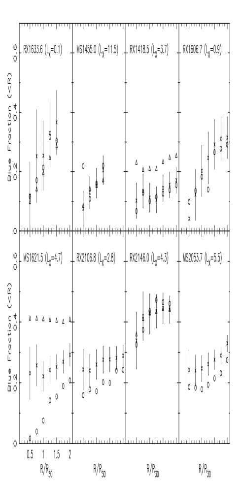
Figure 7: Plot of blue fractions versus radius as a function of $\rm R_{30}$ for the eight clusters presented in this paper. The results shown here are for the $V-R$ and $R-I$ colours for the low and high redshift clusters respectively, corresponding approximately to $B-V$ at rest. Clusters are shown in redshift order, from left to right, with low redshift clusters on the top row. The various symbols represent differing magnitude cuts. Open circles show blue fractions at $\rm M_{v}<-21$, diagonal crosses give $\rm f_{b}$ values for $\rm M_{v}<-20$ and triangles represent $\rm M_{v}<-19$. We give only results in the magnitude ranges in which we believe we are complete and at radii which are completely enclosed within the central CCD. Error bars are given at only one magnitude for clarity. X-ray luminosities are given in units of $\rm 10^{44}\,erg\,s^{-1}$.

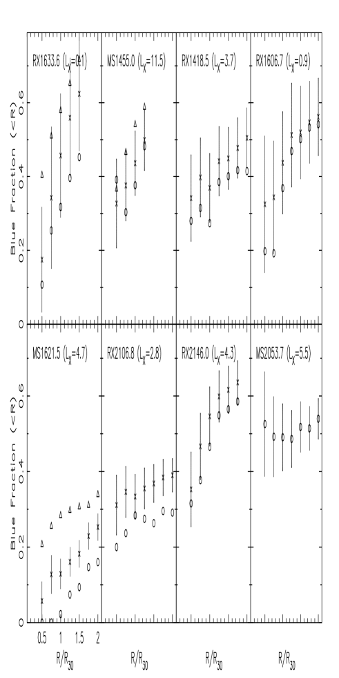
Figure 8: Plot of blue fractions versus radius as a function of $\rm R_{30}$ for the eight clusters presented in this paper. The results shown here are for the $B-V$ and $V-R$ colours for the low and high redshift clusters respectively, corresponding approximately to $U-B$ at rest. Symbols are as in Figure 7.

In Figure 6 we investigate the $\rm f_{b}$ values as a function of X-ray luminosity. We conclude that no real trend can be found, over the factor of 100 or so in X-ray luminosity, though the large errors on the data points makes an expansion of the sample a priority before any rigorous conclusions can be drawn. This result is, however, in agreement with the lack of blue fraction correlation to X-ray luminosity in the ? sample (?; ?). If this result is substantiated, it has important implications for the physical processes that are responsible for the Butcher–Oemler effect.

An interesting question is whether the galaxies within $\rm R_{30}$ would expect to have had their gas removed via ram–pressure stripping due to the ICM (?). An estimate of the dependence of ram–pressure stripping with $L_{x}$ can be made as follows. The rate of ram–pressure stripping is proportional to $\sim\,{\rho}_{\scriptscriptstyle{ICM}}\,{V_{gal}}^{2.4}$ (?) and $L_{x}\,\propto\,{{\rho}_{\scriptscriptstyle{ICM}}}^{2}$. From the Virial theorem and the luminosity–temperature relation, $V_{gal}\,\propto\,T^{0.5}\,\propto\,{L_{x}}^{1/6}$, and so the ram–pressure stripping rate will increase as $\sim\,L_{x}$. Thus the truncation of star–formation by ram–pressure stripping is expected to be significantly more effective in high $\rm L_{x}$ clusters, especially over the factor of 100 in $\rm L_{x}$ sampled here.

? model a large spherical galaxy ploughing through a dense ICM and being stripped of gas. They find that gas stripping is primarily a function of cluster temperature (and hence mass), galaxy velocity within the ICM, the gas replenishment rate from stars and the distance from the centre of the cluster potential. We can make an estimate of cluster mass from our X-ray luminosities via the X-ray luminosity–temperature relation (e.g. ?) which has been shown to be non-evolving for the redshift ranges of our clusters (?; ?). Our most massive cluster, MS1455.0, in which ram–pressure stripping should be most powerful, should have a temperature of approximately 6 keV. We estimate, from predictions presented in Figure 6 of ?, that ram–pressure stripping will only be a dominant force towards the centre of clusters, and then only for luminous, high temperature clusters (i.e. $\rm T_{x}\,\stackrel{{\scriptstyle>}}{{{}_{\sim}}}\,3\,keV$; see also ?). Thus, even if the orbits of most galaxies within $\rm R_{30}$ have taken them close to the cluster centre in the past, we would not expect ram-pressure stripping to be a dominant process in the low $\rm L_{x}$ clusters. To increase the ram-pressure force, we would require that either infalling galaxies have velocities significantly larger than the mean galaxy velocity (which is not inconceivable, e.g. ?), or that the gas replenishment rate is too low to be effective in replacing stripped gas, which may be less plausible. If the excess of blue galaxies in the low X-ray luminosity clusters studied here contains a large fraction of post–starburst galaxies, as found in richer clusters, then a mechanism other than ram–pressure stripping is probably responsible for truncating the star formation.

6.3 Blue fractions with radius and galaxy infall

It has been widely noted that blue fraction varies with cluster–centric radius. To investigate this in our sample we estimate the blue fractions detailed in the previous sections within various radii for each cluster. We consider here both colours and study the variation of $\rm f_{b}$ with radius as a fraction of $\rm R_{30}$. Figures 7 and 8 show plots of integrated blue fraction versus radius, for each of our clusters, in the red and blue colours respectively. We plot the blue fraction at varying magnitude cut–offs, in order to estimate the effect of including brighter or fainter galaxies. As can be clearly seen there is a large variation in the profiles of some of the clusters, a small change in others. In most of the clusters we see an increasing blue fraction with fainter magnitude cut (in agreement with ?). This trend, however, is not universal in our cluster sample. We note also that the slope of $\rm f_{b}$ with radius, for each cluster, is similar in both colours, with the principle difference again being the magnitude of $\rm f_{b}$.

Most of the clusters exhibit at least some increase in blue fraction with radius, which highlights the need for caution when interpreting a blue fraction, at a characteristic radius, for a cluster. However the main conclusions drawn in the previous sections should not vary dramatically given small shifts in characteristic radii. The radius used here, $\rm R_{30}$, is of course dependent on the galaxy distribution. We also investigated the effect of using a radius derived from the X-ray properties of the cluster on the blue fractions. Here we used our estimated cluster temperatures to assign a cluster radius ($\rm r_{200}$), assuming the clusters followed an NFW profile (?). We found that the blue fractions at $\rm r_{200}/2$ were in agreement (within errors) with those at $\rm R_{30}$. This is not too surprising as the galaxy population would be expected to roughly trace the cluster dark matter profile in relaxed clusters.

To what extent are the conclusions drawn from Figures 5 and 6 dependent on the absolute magnitude limit and the radius used to measure the blue fraction? Figures 7 & 8 show that the broad trends of the variation of blue fraction with absolute magnitude, radius and colour are similar from cluster to cluster, so that the conclusions drawn from Figures 5 and 6 are to a large degree independent of the precise choice of absolute magnitude limit or radius, so long as a consistent choice (with radius as a fraction of $\rm R_{30}$) is made.

The increase in blue fraction with radius in many clusters suggests that it is field galaxies falling into the cluster which cause the enhanced blue population (e.g. ?) and which may be one of the prime causes of the well known morphology–density relation, where spiral fraction increases with decreasing galaxy number density (e.g. ?). The mechanism by which the infalling field galaxies are morphologically transformed and have their star formation truncated could be ram–pressure stripping. As discussed in the previous section, the likelihood of ram-pressure stripping increases with ICM density towards the cluster centre. Gas stripping, however, should be less important in the lower luminosity clusters (e.g. RXJ1633.6 and RXJ1606.7). Thus the increase in blue fraction with radius seen in these systems should not be due to ram-pressure stripping.

7 Conclusions

We have presented the first results from a large multi–colour, wide–field imaging program of high redshift X-ray selected clusters. We use the large background area available from our observations of 8 clusters, using the INT WFC, to allow a statistical estimate of the fraction of blue galaxies in the cluster cores. The $B$, $V$, and $R$ band photometry for four intermediate redshift clusters ($z\sim 0.25$) and $V$, $R$ and $I$ band photometry for four higher redshift systems ($z\sim 0.5$), corresponded approximately to $UBV$ at rest.

We find no significant change of blue fraction with redshift in the range 0.2$<$z$<$0.5, but the blue fraction in all the clusters is higher than in those of ? at z$<$0.1. Our reddest colour matches that used by ?. In this colour, the blue fractions we measure are equally consistent (within the measurement errors) with the trend–line presented in ?, or with no trend in blue fraction with redshift at 0.2$<$z$<$0.5. Our blue fractions in this colour are also in agreement with those measured in X-ray selected, luminous clusters by ? over a similar redshift range as used here. However, our blue fractions are higher than those measured in X-ray selected, luminous clusters by ? at z$\approx$0.25. ? find a median blue fraction of $f_{b}=0.04\pm 0.02$ for concentrated clusters ($\rm C>0.35$). A possible explanation lies in the different colour (restframe $U-R$ or observed $B-I$) and selection band (restframe $R$) used by ? to define the blue fraction.

We note a significant difference in the blue fraction values as calculated in our two different colour bands. This may explain some of the scatter in previous blue fraction measurements, which use a variety of different colours, and may additonally imply some level of bias in $\rm f_{b}$, depending on the optical band used for cluster selection.

We find no evidence for a trend in blue fraction with X-ray luminosity, though again our results exhibit a large scatter. Interestingly we do not find the relation between blue fraction and richness that ? find. Unfortunately, whilst that study was based on a large cluster catalogue the authors chose to extract blue fractions at a common fixed spatial radius for each cluster. This obviously prevents direct comparison with this work. It may also explain their richness correlation result, since a lower blue fraction in richer clusters could be due to the smaller radii (relative to $\rm R_{30}$) used to sample the richer clusters, combined with the morphology–density relation.

Profiles of blue fractions with radius show an increasing proportion of blue galaxies, often faint, towards the outskirts of the clusters. The fact that the blue fraction is a function of radius, of faint magnitude cut, and also of the colour used to define it, emphasizes the need for extreme caution when assigning a characteristic blue fraction for an individual cluster. This may provide an explanation for the widely differing blue fraction levels reported in various studies. ?, for example, find a high blue fraction of 0.8 at z=0.9, but use a different method to most studies, employing Stromgren photometry, a variable cluster radius and photometric redshifts to help remove background galaxies. Comparison of blue fractions measured using different techniques may not be valid.

Our results suggest that the increased blue fractions are caused by infalling field galaxies, which may or may not undergo a starburst, before having their star formation truncated. We would expect that ram–pressure stripping occurs in the cores of our more X-ray luminous clusters, and this would cause the lowering of blue fraction, towards the cluster cores, that is observed. This explanation, however, is less likely to explain the same observational result in lower $\rm L_{x}$ systems, where other physical processes (such as galaxy interactions) must be occurring. Our expanded cluster sample will allow a better understanding of the physical processes giving rise to blue galaxies in high redshift clusters.

8 Acknowledgments

We thank Ale Terlevich for his help with the CMR fitting and are grateful for useful discussions with Dave Gilbank regarding INT WFC reduction. De-fringing of data was carried out using the code developed by Mike Irwin and we would also like to thank the Cambridge CASU for providing public access to the WFS calibration details on their website (http://www.ast.cam.ac.uk/$\sim$wfcsur/). We thank the referee for useful comments. Computing facilities provided by the STARLINK project have been used in this work. BWF and DAW acknowledge the receipt of PPARC studentships and LRJ also acknowledges the support of PPARC. DJB acknowledges the support of SAO contract SV4-64008.

References

- [Abadi et al.¡1999¿] Abadi M. G., Moore B., Bower R. G., 1999, MNRAS, 308, 947
- [Abell¡1958¿] Abell G. O., 1958, ApJS, 3, 211
- [Allington-Smith et al.¡1993¿] Allington-Smith J. R., Ellis R. S., Zirbel E. L., Oemler A., 1993, ApJ, 404, 521
- [Andreon & Ettori¡1999¿] Andreon S., Ettori S., 1999, ApJ, 516, 647
- [Balogh et al.¡1997¿] Balogh M. L., Morris S. L., Yee H. K. C., Carlberg R. G., E. E., 1997, ApJ, 488, L75
- [Balogh et al.¡1999¿] Balogh M. L., Morris S. L., Yee H. K. C., Carlberg R. G., E. E., 1999, ApJ, 527, 54
- [Beers et al.¡1990¿] Beers T. C., Flynn K., Gebhardt K., 1990, AJ, 100, 32
- [Bertin & Arnouts¡1996¿] Bertin E., Arnouts S., 1996, A&AS, 117, 393
- [Burke et al.¡1997¿] Burke D. J., Collins C. A., Sharples R. M., Romer A. K., Holden B. P., Nichol R. C., 1997, ApJ, 488, L83
- [Butcher & Oemler¡1978a¿] Butcher H., Oemler A., 1978a, ApJ, 219, 18
- [Butcher & Oemler¡1978b¿] Butcher H., Oemler A., 1978b, ApJ, 226, 559
- [Butcher & Oemler¡1984¿] Butcher H., Oemler A., 1984, ApJ, 285, 426
- [Byrd & Valtonen¡1990¿] Byrd G., Valtonen G., 1990, ApJ, 350, 89
- [Collins et al.¡1997¿] Collins C. A., Burke D. J., Romer A. K., Sharples R. M., Nichol R. C., 1997, ApJ, 479, L117
- [Couch & Sharples¡1987¿] Couch W. J., Sharples R. M., 1987, MNRAS, 229, 423
- [Couch et al.¡1994¿] Couch W. J., Ellis R. S., Sharples R. M., Smail I., 1994, ApJ, 430, 121
- [David et al.¡1993¿] David L. P., Slyz A., Jones C., Forman W., Vrtilek S. D., Arnaud K. A., 1993, ApJ, 412, 479
- [Diaferio et al.¡2001¿] Diaferio A., Kauffmann G., Balogh M. L., White S. D. M., Schade D., E. E., 2001, MNRAS, 323, 999
- [Dressler & Gunn¡1992¿] Dressler A., Gunn J. E., 1992, ApJS, 78, 1
- [Dressler et al.¡1985¿] Dressler A., Gunn J. E., Schneider D. P., 1985, ApJ, 294, 70
- [Dressler et al.¡1994¿] Dressler A., Oemler A., Butcher H., Gunn J. E., 1994, ApJ, 430, 107
- [Dressler et al.¡1997¿] Dressler A. et al., 1997, ApJ, 490, 577
- [Ellingson et al.¡2000¿] Ellingson E., Lin H., Yee H. K. C., Carlberg R. G., 2000, ApJ, 547, 609
- [Ellis et al.¡1997¿] Ellis R. S., Smail I., Dressler A., Couch W. J., Oemler A., Butcher H., Sharples R. M., 1997, ApJ, 483, 582
- [Fairley et al.¡2000¿] Fairley B. W., Jones L. R., Scharf C., Ebeling H., Perlman E., Horner D., Wegner G., Malkan M., 2000, MNRAS, 315, 669
- [Frenk et al.¡1990¿] Frenk C. S., White S. D. M., Efstathiou G., Davis M., 1990, ApJ, 351, 10
- [Fukugita et al.¡1995¿] Fukugita M., Shimasaku K., Ichikawa T., 1995, PASP, 107, 945
- [Gaetz et al.¡1987¿] Gaetz T. J., Salpeter E. E., Shaviv G., 1987, ApJ, 316, 530
- [Gioia & Luppino¡1994¿] Gioia I. M., Luppino G. A., 1994, ApJS, 94, 583
- [Gunn & Gott¡1972¿] Gunn J. E., Gott J. R., 1972, ApJ, 176, 1
- [Gunn et al.¡1986¿] Gunn J. E., Hoessel J. G., Oke J. B., 1986, ApJ, 306, 30
- [Henry & Lavery¡1987¿] Henry J. P., Lavery R. J., 1987, ApJ, 323, 473
- [Ives et al.¡1996¿] Ives D. J., Tulloch S., Churchill J., 1996, SPIE, 2654, 266
- [Jones et al.¡1991¿] Jones L. R., Fong R., Shanks T., Ellis R. S., Peterson B. A., 1991, MNRAS, 249, 481
- [Jones et al.¡1998¿] Jones L. R., Scharf C., Ebeling H., Perlman E., Wegner G., Malkan M., Horner D., 1998, ApJ, 495, 100
- [Kodama & Bower¡2001¿] Kodama T., Bower R. G., 2001, MNRAS, 321, 18
- [Landolt¡1992¿] Landolt A. U., 1992, AJ, 104, 340
- [Lavery & Henry¡1986¿] Lavery R. J., Henry J. P., 1986, ApJ, 304, L5
- [Lavery & Henry¡1988¿] Lavery R. J., Henry J. P., 1988, ApJ, 330, 596
- [Lea & Henry¡1988¿] Lea S. M., Henry J. P., 1988, ApJ, 332, 81
- [Lucey¡1983¿] Lucey J. R., 1983, MNRAS, 204, 33
- [Margoniner & de Carvalho¡2000¿] Margoniner V. E., de Carvalho R. R., 2000, AJ, 119, 1562
- [Margoniner et al.¡2001¿] Margoniner V., de Carvalho R., Gal R., Djorgovski S., 2001, ApJ, 548, L143
- [McMahon et al.¡1999¿] McMahon R. G., Walton N. A., Irwin M. J., Lewis J. R., Bunclark P. S., Jones D. H. P., Sharp R. G. in Instrumentation at the ING, Elsevier Science, 1999
- [Metcalfe et al.¡1991¿] Metcalfe N., Shanks T., Fong R., Jones L. R., 1991, MNRAS, 249, 498
- [Metcalfe et al.¡1995¿] Metcalfe N., Shanks T., Fong R., Roche N., 1995, MNRAS, 273, 257
- [Metevier et al.¡2000¿] Metevier A. J., Romer A. K., Ulmer M. P., 2000, AJ, 119, 1090
- [Moore et al.¡1996¿] Moore B., Katz N., Lake G., Dressler A., Oemler A., 1996, Nature, 379, 613
- [Morris et al.¡1998¿] Morris S. L., Hutchings J. B., Carlberg R. G., Yee H. K. C., Ellingson E., Balogh M. L., Abraham R. G., 1998, ApJ, 507, 84
- [Mushotzky & Scharf¡1997¿] Mushotzky R. F., Scharf C. A., 1997, ApJ, 482, L13
- [Navarro et al.¡1995¿] Navarro J. F., Frenk C. S., White S. D. M., 1995, MNRAS, 275, 720
- [Rakos & Schombert¡1995¿] Rakos K. D., Schombert J. M., 1995, ApJ, 439, 47
- [Scharf et al.¡1997¿] Scharf C., Jones L. R., Ebeling H., Perlman E., Malkan M., Wegner G., 1997, ApJ, 477, 79
- [Schlegel et al.¡1998¿] Schlegel D. J., Finkbeiner D. P., Davis M., 1998, ApJ, 500, 525
- [Smail et al.¡1995¿] Smail I., Hogg D. W., Yan L., Cohen J. G., 1995, ApJ, 449, L105
- [Smail et al.¡1998¿] Smail I., Edge A. C., Ellis R. S., Blandford R. D., 1998, MNRAS, 293, 124
- [Stanford et al.¡1998¿] Stanford S. A., Eisenhardt P. R., Dickinson M., 1998, ApJ, 492, 461
- [Steidel & Hamilton¡1993¿] Steidel C. C., Hamilton D., 1993, AJ, 105, 2017
- [Stevens et al.¡1999¿] Stevens I. R., Acreman D. A., Ponman T., 1999, MNRAS, 310, 663
- [Struble & Rood¡1991¿] Struble M. F., Rood H. J., 1991, ApJ, 374, 395
- [Toomre & Toomre¡1972¿] Toomre A., Toomre J., 1972, ApJ, 178, 623
- [Trentham¡1997¿] Trentham N., 1997, MNRAS, 286, 133
- [Tyson et al.¡1998¿] Tyson J. A. et al., 1998, AJ, 116, 102
- [Vikhlinin et al.¡1998¿] Vikhlinin A., McNamara B. R., Forman W., Jones C., Quintana H., Hornstrup A., 1998, ApJ, 502, 558
- [Yee et al.¡1996¿] Yee H. K. C., Ellingson E., Carlberg R. G., 1996, ApJS, 102, 269