From Correlations of Galaxy Properties to the Physics of Galaxy Formation:
A Theoretical Framework

Abstract

Motivated by forthcoming data from the Sloan Digital Sky Survey, we present a theoretical framework that can be used to interpret Principal Component Analysis (PCA) of disk galaxy properties. We use the formalism introduced by Mo, Mao, & White to compute the observable properties of galaxies in a number of model populations, varying assumptions about which physical parameters determine structural quantities and star formation histories. We then apply PCA to these model populations. Our baseline model assumes that halo mass, spin parameter, and formation redshift are the governing input parameters and that star formation is determined by surface density through a Schmidt law. To isolate physical effects, we consider simplified models in which one of these input parameters is held fixed. We also consider extended models that allow variations in disk mass or angular momentum relative to halo quantities or that choose a star formation timescale independent of surface density. In all cases, the first principal component is primarily a measure of the shape of the spectral energy distribution (SED), and it is usually driven by variations in the spin parameter, which influences star formation through the disk surface density. The second and (in some cases) third principal components consist mainly of “scale” parameters like luminosity, disk radius, and circular velocity. However, the detailed division of these scale parameters, the disk surface brightness, and the rotation curve slope among the principal components changes significantly from model to model. Our calculations yield predictions of principal component structure for the baseline model of disk galaxy formation, and a physical interpretation of these predictions. They also show that PCA can test the core assumptions of that model and reveal the presence of additional physical parameters that may govern observable galaxy properties.

1 Introduction

Recent progress in the empirical understanding of galaxy formation has been driven in large part by evolutionary studies, which can trace changes in the galaxy population over lookback time. The properties of galaxies at the present day, and the correlations among those properties, offer equally important clues to the physical processes that govern galaxy formation. This empirical approach will be revolutionized in the next few years by the Sloan Digital Sky Survey (SDSS; York et al. 2000) and other large imaging and spectroscopic surveys, which provide distances and multi-color photometric information for large samples of galaxies. In statistical analyses of such large data sets, Principal Component Analysis (PCA) is a powerful tool for characterizing correlations among many measurable quantities in terms of a few, independently varying components. If we think of each galaxy as a point in the multi-dimensional space of its observable properties, then PCA yields a compact but highly informative description of the distribution of galaxies in that multi-dimensional space. Applications of PCA to elliptical galaxies have shown that they occupy a thin “fundamental plane” in the space of luminosity, size, and velocity dispersion (Djorgovski & Davis 1987; Dressler et al. 1987; Guzman, Lucey, & Bower 1993). Application to disk galaxies has been more difficult because of the greater difficulty in controlling selection biases for lower surface brightness objects (Disney & Phillipps 1983); however, there are well established bivariate correlations between luminosity and rotation velocity (Tully & Fisher 1977) and between luminosity and surface brightness (de Jong & Lacey 2000; Cross et al. 2001; Blanton et al. 2001). The SDSS will be an ideal target for PCA of all galaxy types. The goal of this paper is to provide a theoretical framework for connecting PCA of disk galaxy properties to the underlying physics that controls disk galaxy formation.

The conventional sketch of disk galaxy formation has its roots in the work of White & Rees (1978) and Fall & Efstathiou (1980), updated and substantially extended by Dalcanton, Spergel, & Summers (1997) and Mo, Mao, & White (1998, hereafter MMW; see also Mao, Mo, & White 1998; Heavens & Jimenez 1999; Mo, Mao, & White 1999; van den Bosch 2000, 2001). A dark matter halo undergoes gravitational collapse and settles into dynamical equilibrium at some formation redshift. The baryonic material within this halo (or some fraction of it) dissipates its energy and settles into a gas disk, preserving its specific angular momentum, and the disk gravity causes the dark halo to contract adiabatically (Blumenthal et al. 1986). The mass of the disk is determined by the halo mass and the cooled baryon fraction, and the size of the disk is determined by the halo virial radius and the halo spin parameter $\lambda$. The initially gaseous disk is converted into stars according to an empirical correlation between surface density and star formation rate (Schmidt 1959; Kennicutt 1998).

Hydrodynamic simulations (e.g., Katz 1992; Navarro & White 1994; Steinmetz & Müller 1994; Domínguez-Tenreiro, Tissera, & Sáiz 1998; Kaellander & Hultman 1998; Weil, Eke, & Efstathiou 1998; Sommer-Larsen, Gelato & Vedel 1999; Navarro & Steinmetz 2000) and “semi-analytic” methods based on halo merger trees (White & Frenk 1991; Kauffmann, White, & Guiderdoni 1993; Cole et al. 1994; Avila-Reese & Firmani 1998; Somerville & Primack 1999) provide more sophisticated models of disk galaxy formation, treating some of the underlying physical processes in greater detail. However, the MMW formalism appears well suited to our purposes here, at least at this initial stage, because it allows easy variation of its input assumptions and relatively straightforward interpretation of its governing parameters. Its principal shortcoming is a highly idealized description of physical processes that are bound to be more complex in a fully realistic calculation. Our present application, though, is relatively undemanding in terms of quantitative accuracy, since we wish to calculate correlations among observable properties but do not consider the zero-points or full distribution functions of these properties.

The “baseline model” of disk galaxy formation that we adopt later in this paper is based on the conventional picture outlined above, and specifically on the version of that picture presented by MMW. However, while MMW set out to calculate and test the predictions of the cold dark matter (CDM) scenario of galaxy formation, making the most reasonable assumptions that could be implemented within their computational framework, we seek instead to understand how departures from the standard assumptions might reveal themselves in the principal components of galaxies’ observable properties. We will therefore compare predictions of the baseline model to those of “extended” models that allow additional variations in physical input parameters or alter the link between galaxy structure and star formation. To clarify the links between governing parameters and predicted correlations, we also consider simplified models in which variation of some input parameters is suppressed. We gain further insight by examining the correlations of principal components with the physical inputs like halo mass, spin parameter, and formation redshift, illustrating the connection between the observables and the “hidden variables” of this theory of galaxy formation.

The next section describes our method of calculating galaxy properties, concluding with a summary of how we go from the physical input parameters to the observable quantities that we use for PCA. Details of the chemical evolution model are presented in an Appendix. In §3 we briefly review the ideas behind PCA. In §4 we present our results for the correlations and principal component structure of the simplified models, the baseline model, and the extended models, with a summary in §4.4. We conclude with a discussion of future directions.

2 Calculation of Galaxy Properties

Our investigation focuses on the population of relatively isolated disk galaxies. The fragility of galactic disks implies that such galaxies must have had fairly quiescent accretion histories (e.g., Toth & Ostriker 1992; Quinn, Hernquist & Fullagar 1993). We therefore adopt the calculational methods of MMW, which consider the settling of gas within a single dark matter halo, rather than a more elaborate method based on halo merger trees. We incorporate star formation and spectral and chemical evolution following (and extending) the techniques of Heavens & Jimenez (1999); similar methods have been employed by van den Bosch (2000, 2001). In real galaxies, the processes of gas dissipation and star formation may be quite complex, especially if feedback from young stars and supernovae plays a major role in regulating gas flow into and out of the forming galaxy. In our calculations, we summarize the effects of these complex processes with a small number of parameters, which characterize, for example, the ratios of disk mass and disk angular momentum to halo mass and halo angular momentum. These parameters, together with parameters that describe the properties of the dark halo itself, define an individual galaxy and allow us to calculate numerous observable properties as described below. In §4, we will consider ten different “models of galaxy formation,” which differ from each other in the distributions adopted for these galaxy input parameters.

2.1 Cosmology

For all of our calculations, we adopt a cosmological model with matter density parameter $\Omega_{m,0}=0.3$, a cosmological constant $\Omega_{\rm\Lambda,0}=0.7$, a Hubble constant $h\equiv H_{0}/100\,{\rm{km\,s^{-1}}}\,{\rm{Mpc}}^{-1}=0.7$, a cold dark matter power spectrum with inflationary index $n=1$ and normalization $\sigma_{8}=1.13$, and a baryon density $\Omega_{b,0}h^{2}=0.0125$ (Burles, Nollett & Turner 2001). The values of cosmological parameters have a limited impact on our calculations. The matter density, cosmological constant, and Hubble constant determine the age of the universe and the relation between time and redshift, which in turn influence the spectral evolution of the galaxies. We adopt the ratio of baryon density to total matter density, $f_{b}\equiv\Omega_{b,0}/\Omega_{m,0}$, as an upper limit on the ratio of galaxy disk mass to halo mass. The amplitude and shape of the matter power spectrum, together with the growth history determined by $\Omega_{m,0}$ and $\Omega_{\rm\Lambda,0}$, determine the distribution of halo masses and the characteristic formation redshift and concentration parameter at each mass. Changes to the cosmological parameters would shift the zero-points of some of our computed correlations between galaxy properties; for example, by changing the ages of stellar populations or the contributions of dark matter to rotation velocities. However, changes within the range allowed by current observations would probably not have much impact on the structure of the principal components.

2.2 Halo Formation

For each dark matter halo, we need to know the mass, the density profile, the total angular momentum, and the formation redshift. In combination with other parameters described later, these determine the mass, size, rotation curve, and star formation history of the corresponding disk.

We draw halo masses from the analytic mass function derived by Press & Schechter (1974, hereafter PS). The comoving number density of dark halos with mass in the range $M_{h}\to M_{h}+dM_{h}$ at redshift $z$ is

$$n_{h}(M_{h},z)dM_{h}=-{{\overline{\rho}}_{0}\over M_{h}}\left({2\over\pi}\right)^{1/2}{\delta_{z}\over\sigma^{2}(r)}\left(\partial\sigma\over\partial M_{h}\right){\rm exp}\left[-{\delta_{z}^{2}\over 2\sigma^{2}(r)}\right]{dM_{h}},$$ (1)

where ${\overline{\rho}}_{0}$ is the mean mass density of the universe at the present time, $\delta_{z}$ is the critical linear overdensity for collapse at redshift $z$, $\sigma$ is the mass variance of linear density fluctuations in top-hat windows of comoving radius $r$, and $M_{h}$ is the average mass inside a sphere of comoving radius $r$. In this paper, we concentrate only on the properties of present-day galaxies, and we therefore draw halo masses from the PS mass function evaluated at $z=0$. However, our galaxy evolution code also computes the properties of galaxy populations at other redshifts.

We assume that $M_{h}$ represents the total mass (dark and baryonic) in a sphere of radius $r_{200}$, within which the mean density is 200 times the critical density. This definition implies a relation between $M_{h}$ and the halo circular velocity at $r_{200}$,

$$M_{h}=\frac{4\pi}{3}200\rho_{\rm crit}r_{200}^{3}=\frac{V_{200}^{3}}{10GH(z)}\ .$$ (2)

In physical units,

$$r_{200}=163\left(\frac{M_{h}}{10^{12}h^{-1}M_{\odot}}\right)^{1/3}\left(\frac{\Omega_{m,0}}{\Omega_{m}(z)}\right)^{1/2}(1+z)^{-1}h^{-1}\,{\rm{kpc}}\ ,$$ (3)

and

$$V_{200}=\biggl{(}{GM_{h}\over r_{200}}\biggr{)}^{1/2}=200\biggl{(}{r_{200}\over 200h^{-1}{\rm kpc}}\biggr{)}\,\biggl{(}{\Omega_{m,0}\over\Omega_{m}(z)}\biggr{)}^{1/2}(1+z)^{3/2}\,{\rm km/s}\ .$$ (4)

We truncate the PS mass function at $V_{200}<40\,{\rm{km\,s^{-1}}}$ (at $z=0$), in part to restrict our attention to the range of luminosities where the disk galaxy population is best characterized observationally and in part because photoionization heating by the cosmic UV background is likely to have an important influence on the collapse and cooling of gas within lower mass halos (Thoul & Weinberg 1996; Quinn, Katz, & Efstathiou 1996; Gnedin 2000). We also truncate the mass function at $V_{200}>300\,{\rm{km\,s^{-1}}}$, since disk galaxies with rotation velocities larger than $300\,{\rm{km\,s^{-1}}}$ are rare. No doubt some disk galaxies do reside within more massive halos, but these are the common halos of groups that contain multiple galaxies, and our present calculational approach (which assumes one galaxy per halo) cannot be applied to them.

We assume that each halo has a density profile of the form proposed by Navarro, Frenk, & White (1997, hereafter NFW; see also Navarro, Frenk & White 1995, 1996), which has asymptotic logarithmic slopes of $-1$ in the central regions (as found by Dubinski & Carlberg 1991; Warren et al. 1992) and $-3$ in the outer regions. The transition between these regimes occurs at a scale radius $r_{s}$, and the shape of the profile can be characterized by the dimensionless concentration parameter $c\equiv r_{200}/r_{s}$. If we adopted the profile form suggested by Moore at al. (1999), which has an asymptotic inner slope of $-1.5$, we would generally predict higher circular velocities and flatter rotation curve slopes for a given galaxy luminosity, though again we would expect this change to affect mainly the zero points of relations rather than the overall structure of principal components.

The central densities of halos are connected to the physical density of the universe at the time that they assemble. Concentrations therefore tend to be higher in cosmologies with lower $\Omega_{m,0}$ or larger mass fluctuation amplitudes, since these changes shift halo formation to higher redshifts. In any given cosmology, average halo concentrations are higher for less massive halos, which tend to collapse earlier. Jing (2000) and Bullock et al. (2001b) find that there is also significant scatter in concentrations at a given mass, with a distribution of concentrations that is roughly log-normal with a scatter $\sigma_{\ln c}\approx 0.2$. In all of our calculations, we take the mean concentration $\bar{c}$ as a function of halo mass from Table 2 of Jing (2000). In some models, we also include a log-normal scatter in concentrations, taking $\sigma_{\ln c}$ from the same source. For the star formation calculations described in §2.4, we need to compute the disk scale length as a function of redshift, which in turn depends slightly on the halo concentration as a function of redshift. Based on the numerical results of Bullock et al. (2001b), we assume that the concentration parameter evolves as $c\propto(1+z)^{-1}$.

The angular momentum of the halo is characterized by the dimensionless spin parameter, $\lambda$, defined as (Peebles 1993)

$$\lambda=\frac{J_{h}|E|^{1/2}}{GM_{h}^{5/2}},$$ (5)

where $E$ is the halo’s total binding energy and $J_{h}$ is the halo angular momentum, which is usually assumed to originate from tidal torques on the quadrupole moment of the halo near the time of maximum expansion (Peebles 1969). Analytic and numerical studies by several authors (Barnes & Efstathiou 1987; Warren et al. 1992; Catelan & Theuns 1996a, b) find the distribution of spin parameters of collapsed dark matter halos to be well characterized by a log-normal distribution. Most authors find that this distribution peaks at $\overline{\lambda}\approx 0.05$ with a logarithmic width of $\sigma_{\ln\lambda}\approx 0.5$ (MMW, but see also Dalcanton et al. 1997), and that there is little if any correlation between $\lambda$ and halo mass or initial peak height (Barnes & Efstathiou 1987; Ryden 1988). For most of our calculations, therefore, we draw the values of $\lambda$ from a log-normal distribution with these parameters and assume that they are independent of mass and redshift. We will also consider some models in which all halos have $\lambda=\bar{\lambda}$. As discussed in §2.3 below, we will usually follow the conventional assumption (Fall & Efstathiou 1980) that the baryons have the same specific angular momentum as the dark halo and conserve that angular momentum during disk formation, so that the value of $\lambda$ effectively determines the size of the disk. In some models, we will also allow for the possibility that baryons lose angular momentum to the dark matter during collapse.

With the assumption that disks have the same specific angular momentum as their halos, Syer, Mao, & Mo (1999) derive a $\lambda$ distribution from Mathewson & Ford’s (1996) sample of 2500 late-type spiral galaxies that is in good agreement with numerical predictions for halos: log-normal with $\bar{\lambda}=0.05$ and $\sigma_{\ln\lambda}=0.36$ (see de Jong & Lacey 2000 for a similar analysis). Thus, even if the physical process that determines disk sizes is considerably more complicated than the simple picture of collapsed baryons retaining the same specific angular momentum as the parent halo, the conventional assumption provides a good phenomenological description of the observed distribution of disk sizes. The fact that the inferred $\lambda$ distribution is narrower than the predicted one might reflect selection biases against low surface brightness galaxies (large $\lambda$) and compact galaxies (small $\lambda$); the latter may become earlier type galaxies as a result of secular bulge formation.

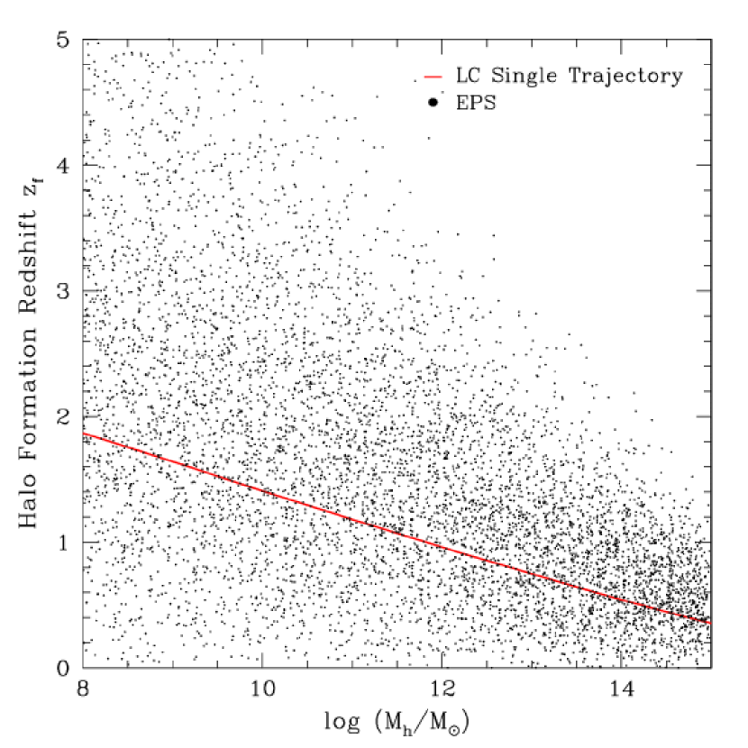
Figure 1: Halo formation redshifts, defined as the half-mass assembly redshift and calculated by the methods of Lacey & Cole (1993). Points show a Monte Carlo realization of the probability distribution of formation redshifts at different halo masses. In models where we suppress the scatter in formation redshifts, we apply the LC “single trajectory” relation shown by the solid line. Our models assume that disk star formation begins at the halo formation redshift.

To calculate the star formation history and spectral evolution of a galaxy, as described in §§2.4 and 2.5 below, we need to know when the star formation in the galaxy begins. We have decided to identify the epoch of initial star formation with the halo formation redshift, which we take to be the time when half of the halo’s final mass has been assembled. These formation redshifts can be computed approximately within the Extended Press-Schechter (EPS) formalism (Bond et al. 1991; Bower 1991), as described by Lacey & Cole (1993) (hereafter LC). In some of our models, we assume that all halos of a given mass have the same formation redshift, and in these cases we use the value implied by equation 2.23 of LC. In other models, we incorporate the full distribution of formation redshifts at fixed halo mass predicted by the EPS formalism, using the prescription in §2.5.2 of LC (equation 2.26 in particular; see the appendix of Kitayama & Suto 1996 for useful approximations). Figure 1 shows the relation between formation redshift and halo mass obtained from the deterministic relation (solid line) and the probabilistic description (points). Clearly there is an overall trend for more massive halos to collapse at later times. However, in the probabilistic model, the scatter in formation redshifts is large in comparison to this trend.

Our identification of the start of star formation with the half-mass assembly epoch of the halo is, of course, somewhat arbitrary. Changes to this prescription would shift the ages of the stellar populations and hence the predicted colors of our model galaxies. From the point of view of our PCA calculations, the important features of this prescription are not its details but the moderate trend of decreasing formation redshift with increasing halo mass, and the substantial scatter in formation redshifts in the probabilistic case. The second of these seems likely to be present in any realistic model, and the amplitude of scatter predicted by halo formation arguments seems like a reasonable guess at the actual scatter in initial star formation epochs. The reality of the trend with mass is less obvious, since one could imagine that stars begin to form in sub-units that assemble into the final galaxy, and that these sub-units form earlier in systems that are fated to become more massive. However, our implicit model is that disk stars form from gas that settles in the halo only after it has completed most of its growth, since major mergers would disrupt a pre-existing disk, and within this picture a trend like that in Figure 1 is plausible. In any event, we will find that the formation redshift plays a sub-dominant role in determining galaxy spectral properties, which are more sensitive to the disk surface density, and thus to the spin parameter $\lambda$.

2.3 Disk Formation

After the gravitational collapse of a dark halo and its associated baryonic material, gas begins to cool and decouple from the dark matter. Since the gas can radiate energy but cannot easily rid itself of angular momentum, it settles into a centrifugally supported disk, rotating in the combined gravitational potential of the halo and the disk itself. Following MMW, we define $m_{d}=M_{d}/M_{h}$ to be the ratio of the disk mass to the total mass $M_{h}$ within the halo virial radius. In a spherical collapse picture, $m_{d}$ should not exceed the universal baryon fraction $f_{b}=\Omega_{b,0}/\Omega_{m,0}$; 3-dimensional hydrodynamic simulations show that cooled gas fractions can sometimes exceed this limit, but not by a large factor (Gardner et al., in preparation; Berlind et al., in preparation). Observational analyses imply that the mean value of $m_{d}$ is substantially less than $f_{b}$, probably by a factor of two or more, though uncertainties in disk mass-to-light ratios and cosmological parameters make estimates quite uncertain (see, e.g., Fukugita, Hogan, & Peebles 1998; Syer, Mao, & Mo 1999). The value of $m_{d}$ is presumably controlled by a combination of cooling physics and feedback processes. If the interaction between cooling and feedback is tightly self-regulated, we might expect the distribution of $m_{d}$ to be narrow. If these processes have large stochastic variations from galaxy to galaxy, the distribution of $m_{d}$ could be broad. We will consider both possibilities: models in which $m_{d}$ is fixed at $0.5f_{b}$ and models in which $m_{d}$ is uniformly distributed in the range $(0,f_{b}]$.

We assume that the cooled baryons settle into an exponential disk, with surface density profile

$$\Sigma(r)=\Sigma_{0}\exp\left(-r/r_{d}\right)=\frac{M_{d}}{2\pi r_{d}^{2}}\exp\left(-r/r_{d}\right).$$ (6)

We compute the scale radius $r_{d}$ by requiring centrifugal support. If the halo were isothermal, the disk had the same specific angular momentum as the halo, and the self-gravity of the disk were negligible, the implied disk scale length would be $r_{d}=\lambda r_{200}/\sqrt{2}$ (MMW). In most of our models, we assume that the specific angular momentum of the disk is the same as that of the halo, implying $j_{d}\equiv J_{d}/J_{h}=m_{d}$. However, we also consider models with angular momentum loss, choosing $j_{d}$ uniformly in the interval $(0,m_{d}]$. Following MMW, we account for the disk’s self-gravity and include the influence of the disk on the dark halo by assuming that the halo contracts adiabatically as the disk forms. The adiabatic contraction condition implies that a halo particle initially at a mean radius $r_{i}$ will end up at a mean radius $r$ such that

$$r_{i}\,M_{i}(r_{i})=r\,M_{f}(r),$$ (7)

where $M_{i}(r)$ is the initial mass distribution given by the NFW density profile and

$$M_{f}(r)=M_{d}(r)+(1-m_{d})M_{i}(r_{i})$$ (8)

is the final mass of the system within $r$ (Blumenthal et al. 1986). $M_{d}(r)$ is the disk mass within $r$ and is explicitly given by

$$M_{d}(r)=M_{d}\biggl{[}1-\Bigl{(}1+{r\over r_{d}}\Bigr{)}\exp(-r/r_{d})\biggr{]}.$$ (9)

Under these conditions, MMW derived the following expressions for the total disk angular momentum and disk scale length:

$$J_{d}=j_{d}J_{h}=\frac{2M_{d}r_{d}V_{200}}{f_{R}},$$ (10)

$$r_{d}={1\over\sqrt{2}}\left({j_{d}\over m_{d}}\right)\lambda r_{200}f_{c}(c)^{-1/2}f_{R}(\lambda,c,m_{d},j_{d}),$$ (11)

$$f_{R}(\lambda,c,m_{d},j_{d})=2\left[\int_{0}^{\infty}e^{-u}u^{2}~{}{V_{c}(r_{d}u)\over V_{200}}~{}du\right]^{-1}\ ,$$ (12)

$$f_{c}(c)={c\over 2}~{}{1-1/(1+c)^{2}-2\ln(1+c)/(1+c)\over[c/(1+c)-\ln(1+c)]^{2}}\ .$$ (13)

The factors $f_{R}$ and $f_{c}$ represent the necessary corrections to be made to quantities such as the disk scale length once the disk self-gravity and halo concentration are taken into account. In particular, $f_{c}$ represents the change in binding energy from a singular isothermal sphere profile to an NFW profile, while the factor $f_{R}$ is associated with both the density profile and the gravitational effects of the disk. Note that the concentrations in equations (11)-(13) depend on redshift, with $c\propto(1+z)^{-1}$ for a given halo.

The rotation curve of the system is obtained by adding in quadrature the contributions from the halo and the exponential disk. Before adiabatic contraction, the halo is described by an NFW profile, and its circular velocity profile can be expressed in terms of the concentration parameter:

$$V_{c}(r)=V_{200}\sqrt{\frac{\ln(1+cx)-(cx)/(1+cx)}{x\ln(1+c)-c/(1+c)}},$$ (14)

where $x=r/r_{200}$. The rotation curve produced by an NFW profile increases as $r^{1/2}$ at small $r$, reaches a maximum at $r/r_{200}\approx 2/c$, and declines beyond this radius. The exponential disk contribution to the rotation curve is (Freeman 1970)

$$V_{d}^{2}(R)=4\pi G\Sigma_{0}r_{d}y^{2}\left[{\cal I}_{0}(y){\cal K}_{0}(y)-{\cal I}_{1}(y){\cal K}_{1}(y)\right]\ ,~{}~{}~{}~{}~{}~{}y\equiv{r\over 2r_{d}}\ ,$$ (15)

where ${\cal I}_{n}$ and ${\cal K}_{n}$ are modified Bessel functions of the first and second kinds. The disk rotational velocity peaks at $r/r_{d}\approx 2.2$, where $V_{d}\approx 0.88\sqrt{\pi G\Sigma_{0}r_{d}}$.

To calculate the rotation curve of the final system, we must obtain $r_{d}$ and compute the influence of adiabatic contraction on the halo contribution. Given values of the halo mass $M_{h}$, spin parameter $\lambda$, and concentration $c$, and the disk mass and angular momentum fractions $m_{d}$ and $j_{d}$, we calculate a first guess at $r_{d}$ using equation (11) with $f_{R}=1$. We then compute the adiabatic contraction caused by a disk with this scale length, solving for $r_{i}$ as a function of $r$ using equations (7)–(9) and thus obtaining $M_{f}(r)$. We then calculate the rotational velocity profile $V_{c}(r)$ and use it in equation (12) to obtain a new value of $f_{R}$, and hence a new estimate of $r_{d}$ to be used in a second iteration. This procedure converges rapidly, returning a value of $r_{d}$ to an accuracy better than one percent in a few iterations.

We characterize the amplitude of our model rotation curves by $V_{2.2}=V_{c}(2.2r_{d})$, the value of the circular velocity at the radius where the disk contribution peaks. For observed galaxies, $V_{2.2}$ is usually close to the velocity used in studies of the Tully-Fisher (1977) relation. As emphasized by Persic, Salucci, & Stel (1996), the shape of the rotation curve is a valuable diagnostic for the halo profile and the relative importance of baryon and dark halo contributions. We characterize the shape by the logarithmic slope of $V_{c}(r)$ between 2 and 3 disk scale lengths,

$$S_{a,b}\equiv\frac{\Delta\log V_{c}}{\Delta\log r}\equiv\frac{\log[V_{c}(3r_{d})/V_{c}(2r_{d})]}{\log(3/2)}.$$ (16)

It is worth noting that the “optical radius” of an exponential disk is $R_{\rm opt}=3.2r_{d}$, corresponding to the de Vaucouleurs $25\;B$ mag arcsec^-2 photometric radius for a typical value of the central surface brightness of $I_{0}=150L_{\odot}\;{\rm pc}^{-2}$. Most well observed galaxy rotation curves extend beyond 3 disk scale lengths (Persic, Salucci, & Stel 1996; Swaters, Madore & Trewhella 2000).

2.4 Star Formation

The star formation rate (SFR) in observed galaxies is tightly correlated with the local gas surface density, a relation that can be approximately characterized by a power law (Schmidt 1959) with a minimum threshold for active star formation (Kennicutt 1989, 1998). Kennicutt (1998) finds that the star formation rates of disk galaxies are well described by the relation

$$\Sigma_{\rm SFR}=A\left({\Sigma_{\rm gas}\over M_{\odot}{\rm pc}^{-2}}\right)^{n},$$ (17)

where $\Sigma_{\rm SFR}$ and $\Sigma_{gas}$ represent the disk-averaged SFR and gas densities, $A=(2.5\pm 0.7)\times 10^{-4}{\rm M_{\odot}yr^{-1}kpc^{-2}}$, and $n=1.4\pm 0.15$.

To derive star formation histories of our disks, we draw on the analytic results of Heavens & Jimenez (1999), and we thus adopt the model of disk evolution that is implicit in their calculations: an exponential gas disk forms at initial redshift $z_{i}$, which we identify with the halo formation redshift $z_{f}$, and this gas is converted into stars at the rate implied by equation (17). The scale length of the disk is determined by the values of $\lambda$ and the virial radius. With this model, Heavens & Jimenez (1999) derived the time evolution of the gas surface density in terms of the initial gas surface density $\Sigma_{i,{\rm gas}}$:

$$\Sigma_{\rm gas}(t)=\left(\Sigma_{i,{\rm gas}}^{-0.4}+0.4Bt\right)^{-2.5}\ ,$$ (18)

where $B=9.5\times 10^{-17}$ in SI units and $t$ is the time elapsed since the initial redshift $z_{i}$. Integrating equation (18) over the entire exponential disk yields the overall star formation rate and remaining gas mass as a function of time:

$$\dot{M}_{\star}(t) = \frac{50\pi Br_{d}^{2}\Sigma_{0}^{1.4}}{49}\phantom{I}_{3}F_{2}\left(3.5,3.5,3.5;4.5,4.5;-a\right)\ M_{\odot}{\rm yr}^{-1},$$ (19)

$$M_{g}(t) = {2\pi r_{d}^{2}\Sigma_{0}}\phantom{I}_{3}F_{2}\left(2.5,2.5,2.5;3.5,3.5;-a\right)\ M_{\odot},$$ (20)

where $\!\phantom{I}{}_{3}F_{2}$ is a generalized hypergeometric function (Gradshteyn & Ryzhik 1980), $r_{d}$ is the disk scale length, and $\Sigma_{0}=M_{d}/2\pi r_{d}^{2}$ is the central gas surface density. The quantity $a$ is a time-like variable defined by

$$a=1.06h_{z}^{0.4}\left({t\over\rm Gyr}\right)\left({V_{200}\over 250\,{\rm{km\,s^{-1}}}}\right)^{0.4}\left({\lambda\over 0.05}\right)^{-0.8}\left({m_{d}\over 0.05}\right)^{0.4}\left({j_{d}\over m_{d}}\right)^{-0.8}f_{c}^{\ 0.4}\ f_{R}^{-0.8},$$ (21)

where $h_{z}\equiv H(z)/100$ km s^-1 Mpc^-1. Heavens & Jimenez (1999) assumed $j_{d}=m_{d}$, an isothermal halo, and no disk self-gravity or adiabatic contraction of the halo. Equation (21) differs from their equation (9) by the inclusion of the last three factors, which account, respectively, for angular momentum loss, NFW halo profiles, and the influence of self-gravity and adiabatic contraction on the disk scale length. Heavens & Jimenez (1999) use the values of $r_{d}$, $\Sigma_{0}$, and $h_{z}$ determined at the formation redshift, thus implicitly assuming that the disk forms with its full mass $M_{d}=m_{d}M_{h}$ at $z=z_{f}$ with size proportional to the halo virial radius at that redshift. In order to approximately treat the growth of the disk over time, we use the time-dependent values of $r_{d}$, $\Sigma_{0}$, $h_{z}$, and $c$ in equations (19)-(21), assuming that the halo evolves at constant circular velocity $V_{200}$ and thus has $M_{d}(z)=m_{d}M_{h}(z)\propto H^{-1}(z)$ and $r_{d}\propto H^{-1}(z)$ (see eq. 2). This treatment is intermediate between assuming that the disk size is determined at $z_{f}$ and assuming that it is determined at $z=0$.

This calculation of a disk’s star formation history is clearly idealized and approximate. However, it is two basic features of this prescription that are crucial to our results. The first is that the gas surface density is the primary physical parameter that controls the speed at which gas converts into stars. The second is that the formation redshift of the halo determines the initiation of star formation.

As an alternative to our standard models, we also create realizations of the galaxy population in which the gas surface density does not drive the SFR. For these models, we assume an exponentially decaying star formation rate with the decay time $\tau$ drawn from a uniform distribution in the interval $[1,9]{\rm\,Gyr}$, independent of the surface density. The disk mass again grows as $M_{d}(z)=m_{d}M_{h}(z)$, starting at the halo formation redshift, and gas added to the disk at time $t_{a}$ is converted into stars at a rate ${\rm SFR}\propto\exp[-(t-t_{a})/\tau]$, with the constant of proportionality chosen so that all of the gas would be consumed as $t\longrightarrow\infty$. In these exponential decline models, the star formation history is decoupled from structural quantities like the spin parameter $\lambda$ and the disk mass fraction $m_{d}$. They provide valuable insight into the origin of the principal component structure of our standard models and show how that structure would change if star formation is not tightly coupled to the surface density over the full history of the disk.

2.5 Spectral and Chemical Evolution

Given the star formation histories calculated above, we compute the spectral evolution of the stellar populations using the current version of the Bruzual & Charlot (2001) spectrophotometric population synthesis (SPS) code. These calculations return observational quantities that play a central role in our principal component analysis, such as broad band magnitudes and colors, stellar mass-to-light ratios, and the strength of the 4000Å spectral break. We implement a fully consistent chemical enrichment model that makes use of the latest Bruzual & Charlot (2001) SPS models and of metallicity dependent lifetimes and yields. We describe the details of this chemical enrichment model in the Appendix.

In all of our evolutionary calculations, we assume that the stellar initial mass function (IMF) has the form proposed by Salpeter (1955), with a logarithmic slope $x=1.35$ over the mass range $m_{l}=0.1M_{\odot}$ to $m_{u}=125M_{\odot}$. Changes to the lower cutoff (or to the form at low masses) would alter the stellar mass-to-light ratios but have little impact on spectral properties, since low mass main sequence stars contribute much of the mass but little of the light for a typical stellar population. Changes to the upper cutoff would influence the enrichment history, since the most massive stars contribute significantly to heavy element production. Changes to the slope in the regime $\sim 1-10M_{\odot}$ would have the most important impact on spectral properties, though even these changes would tend to shift colors in a coherent way without altering the degree of correlation between colors and other galaxy properties. From the point of view of PCA predictions, the key assumption is not the particular form of the IMF but that it is universal, at least when averaged over a galaxy’s history.

2.6 Summary: Inputs and Outputs

In our calculations, an individual galaxy is defined by six input parameters, or seven in the case where the star formation timescale is chosen independently of the surface density. The ten galaxy formation models that we examine in §4 differ in the distributions of these input parameters: which ones are held fixed at typical values and which ones are allowed to vary and therefore play a role in governing the distribution of galaxy properties.

The input parameters (listed in Table 1) are the halo mass $M_{h}$, the halo concentration parameter $c$, the halo spin parameter $\lambda$, the halo formation redshift $z_{f}$, the ratio of disk mass to halo mass $m_{d}=M_{d}/M_{h}$, the ratio of disk angular momentum to halo angular momentum $j_{d}=J_{d}/J_{h}$, and (in some models) the $e$-folding time of the star formation rate $\tau$. The values of $M_{h}$ and $m_{d}$ determine the disk mass. The disk scale length is determined by the condition of centrifugal support in the combined potential well of the disk and the adiabatically contracted halo, so it depends on $M_{h}$ (which fixes the halo virial radius), $\lambda$, and $j_{d}/m_{d}$, and, more weakly, on $c$ and $m_{d}$. Given the size and mass of the disk and the profile of the adiabatically contracted halo, we compute the rotation curve as described in §2.3. The size and mass of the disk also determine the surface density profile, which we use to compute the star formation history as described in §2.4, except in models where we choose the timescale $\tau$ independently of surface density. The halo formation redshift $z_{f}$ also influences the star formation history by defining the initial epoch of star formation. Given the star formation history, we compute spectral and chemical evolution of the galaxy as described in §2.5 and the Appendix.

The results of PCA will depend to a large extent on what observables we choose to incorporate into the analysis. Of the large number of observables that can be computed by our code, we have chosen to work with the set listed in Table 2. These fall roughly into two categories, quantities that describe the scale or structure of the galaxy and quantities that describe the shape of the spectral energy distribution (SED). The first category includes the I-band disk luminosity $L_{d,I}$, the exponential scale length $r_{d}$, the circular velocity at 2.2 disk scale lengths $V_{2.2}$, the rotation curve slope $S_{2,3}$, and the I-band central surface brightness $\mu_{0,I}$. Since we assume that the disk is exponential, the central surface brightness is determined by the luminosity and the scale length, but it proves helpful to treat it as a separate observable because of its direct connection (in Schmidt-law models) to the star formation history. We also include the disk stellar mass $M_{\star}$ and the I-band stellar mass-to-light ratio $(M/L)_{I}$ as observables. In most galaxies it is not possible to measure the stellar mass dynamically, but one can infer a galaxy’s stellar mass-to-light ratio by population synthesis modeling of the SED and multiply by the luminosity to infer a stellar mass, albeit with some uncertainties. While $M_{\star}$ is determined by $L_{d,I}$ and $(M/L)_{I}$ in such an analysis, it is still helpful to treat it as a separate observable in PCA to distinguish between the effects of disk mass and the effects of stellar population on the I-band luminosity.

For the SED observables we have selected three broad-band colors that probe somewhat different features of the stellar population, $(U-B)$, $(B-V)$, and $(V-K)$, and the strength of the 4000Å break $B_{4000}$. We also include the “birth parameter” $b$ (Scalo 1986), the ratio of the galaxy’s current star formation rate to its time-averaged star formation rate:

$$b(t)=\frac{{\rm SFR}(t)}{\langle{\rm SFR}\rangle}\approx\frac{{\rm SFR}(t)\times t}{M_{\star}(t)}\ .$$ (22)

As shown by Bruzual & Charlot (1993), the SED of a model galaxy is usually highly correlated with $b$, even for different overall star formation histories. It therefore serves us both as a scaled characterization of ongoing star formation and as an SED quantity. Our final observable is the mean metallicity $[{\rm Fe/H}]$.

3 Principal Component Analysis

Principal Component Analysis is among the oldest and best known of the techniques of multivariate analysis. It was first introduced by Pearson (1901) and developed independently by Hotelling (1933). The central idea behind PCA is to reduce the dimensionality of a data set in which there are a large number of interrelated variables, while retaining as much as possible of the variation of the whole data set. This reduction is achieved by transforming to a new set of variables, the principal components (hereafter PCs), which are uncorrelated and are ordered so that the first few retain most of the variation present in all the original variables.

Algebraically, PCs are particular linear combinations of the $p$ variables. Geometrically, these linear combinations represent the selection of a new coordinate system obtained by rotating the original system with ${\bf x}=x_{1}$, $x_{2}\ldots x_{p}$ as the coordinate axes. The new axes represent the direction of maximum variability and provide a simpler description of the covariance structure.

We seek to find some new variables $\xi$ = $\xi_{1}$, $\xi_{2}\ldots\xi_{p}$ which are linear functions of the $x$’s but are themselves uncorrelated. In fact, we look for $p^{2}$ constants ${\bf l}=l_{ij}(i,j=1,\ldots,p)$ such that

$${\bf\xi=l\ x}\ ,$$ (23)

with the orthogonality condition ${\bf ll^{\prime}=I}$, where I is the identity matrix. It can be shown (Murtagh & Heck 1987) that if $\bf\Sigma$ is the variance-covariance matrix of the original ${\bf x}$ vector of $p$ variables, then the axis along which the variance is maximal is the eigenvector ${\bf e_{1}}$ of the matrix equation

$${\bf\Sigma e_{1}}=\lambda_{1}{\bf e_{1}},$$ (24)

where $\lambda_{1}$ is the largest eigenvalue, which is in fact the variance along the new axis. The other eigenvalues obey similar equations. The total population variance is then

$$\sigma_{11}+\sigma_{22}+\cdots\sigma_{pp}=\lambda_{1}+\lambda_{2}+\cdots\lambda_{p},$$ (25)

and hence the proportion of total variance explained by the $k$th principal component is

$$\frac{\lambda_{k}}{\lambda_{1}+\lambda_{2}+\cdots\lambda_{p}}\ \ \ \ \ \ \ \ \ \ \ k=1,2,\ldots,p\ .\\$$ (26)

Thus, the first axis accounts for as much of the total variance as possible; the second axis accounts for as much of the remaining variance as possible while being uncorrelated with the first axis; the third axis accounts for as much of the total variance remaining after that accounted for by the first two axes, while being uncorrelated with either, and so on. If most of the total population variance can be attributed to the first few components, then these components can replace the original $p$ variables without much loss of information. The magnitude of each of the $e_{ki}$ eigenvector coefficients measures the importance of the $k$th variable of the $i$th principal component, irrespective of other variables.

It is common (and advisable) to remove any variance introduced only by the widely differing dynamic ranges in variable measures. This is particularly important in our own case when we perform PCA on quantities with measurement units that are not commensurate (see Table 2). We will therefore transform our original variables into a new set with zero mean and unit variance. In matrix notation:

$${\bf z}=({\bf V^{1/2}})^{-1}({\bf x-\mu})$$ (27)

where ${\bf V^{1/2}}$ is the diagonal standard deviation matrix. The PCs of ${\bf z}$ can then be obtained from the eigenvectors of the $correlation$ matrix ${\bf\Theta}=({\bf V^{1/2})\Sigma(V^{1/2})^{-1}}$ of ${\bf x}$. All our previous results still apply, with some simplification since the variance of each $z_{i}$ is now unity. Furthermore, since the total variance is now $p$, equation (26) becomes:

$$\frac{\lambda_{k}}{p}\ \ \ \ \ \ \ \ \ \ \ k=1,2,\ldots,p\ .$$ (28)

The PCs derived from ${\bf\Sigma}$ are, in general, not the same as the ones derived from ${\bf\Theta}$.

In addition to scaling input variables to unit variance, for quantities that characterize size, mass, or velocity scales we take logarithms of observables prior to applying PCA, as indicated by the notations in Table 2. Specifically, we use $\log L_{d,I}$, $\log r_{d}$, $\log V_{2.2}$ and $\log M_{\star}$ (the central surface brightness $\mu_{0,I}$ is in magnitude units and therefore already logarithmic). Logarithmic measures reduce the very large dynamic range in these quantities, and the observed power-law correlations between these quantities translate into linear correlations in their logarithms, making the logarithmic measures more appropriate to the linear analysis of PCA.

Once the PCs have been determined, attention must focus on the relationship of the PCs to the original variables. In order to do so, we first need to address the problem of the number of PCs to retain for further analysis. One rule for determining how many PCs to retain was proposed by Kaiser (1960). The idea behind this rule is that if all elements of ${\bf x}$ are independent, then the PCs are the same as the original variables, and all have unit variances. Thus any PC with variance less than one contains less information than one of the original variables, and so it is not worth retaining. It can be argued that Kaiser’s rule retains too few variables in the case where there are a few variables that are more-or-less independent of all others. These variables, in fact, will have small coefficients in some of the PCs, but will dominate others, whose variance will be close to one. Since these variables provide independent information from the other variables it would be unwise to ignore them. Based on simulations, Jolliffe (1972) proposed to lower the variance threshold to 0.7.

The galaxy formation models below offer a natural, physically motivated choice for the number of PCs to retain in our theoretical analyses: the number of physically significant PCs should equal the number of independently varying input parameters in the model. In every case but one, we find that this choice also corresponds to the number of PCs above a variance threshold of 0.7.

4 The Principal Component Structure of Model Galaxy Populations

Table 3 lists the input parameter values (or distributions) for the ten models of galaxy formation that we study in this section. For each model, we construct a realization of $\sim 500$ disk galaxies evolved to $z_{0}=0$. We compute the quantities listed in Table 2 for each galaxy and apply PCA to these 500 vectors of 13 observables. Models 1 and 2.1-2.5 are deliberately simplified models, with the expected physical variation in one or more input parameters suppressed so that we can isolate the physical effects of others. We discuss these models in §4.1. Model 3 represents our baseline model of galaxy formation, which incorporates variations in $M_{h}$, $\lambda$, and $z_{f}$. We discuss this model in §4.2. Models 4.1-4.3 are extended models, where some additional physical variation is added to the baseline model. We designate those input parameters that vary (i.e., are drawn from a probability distribution rather than fixed to a typical value) as a model’s control parameters. Thus, our models of galaxy formation differ in which control parameters govern the variations in galaxies’ observable properties.

4.1 Simplified Models

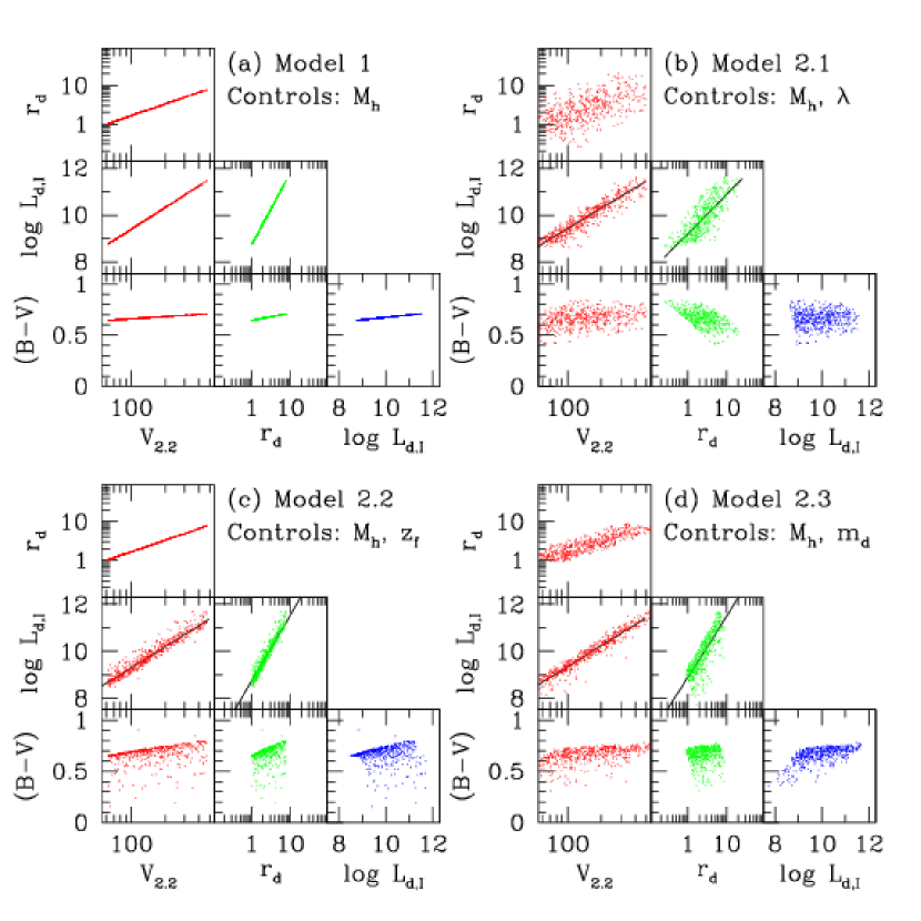
Figure 2: Bivariate correlations among disk rotation velocity (at $2.2r_{d}$), scale length, I-band luminosity, and $\bv$ color in models with one or two control parameters. Galaxies in Model 1 form a 1-parameter family, controlled entirely by halo mass $M_{h}$, so there is no scatter in the correlations. Models 2.1, 2.2, and 2.3 incorporate scatter in the spin parameter $\lambda$, formation redshift $z_{f}$, and disk mass fraction $m_{d}$, respectively, which adds scatter to the bivariate relations and in some cases changes their slopes. Lines in the $L-V$ and $L-r_{d}$ panels show least squares fits to the data points.

Figure 2 presents bivariate correlations among four observables, $V_{2.2}$, $r_{d}$, $L_{d,I}$, and $\bv$, for four of our simplified models. Model 1, shown in Figure 2a, has halo mass $M_{h}$ as the only control parameter. Since the galaxies in this model form a 1-parameter family, the correlations among the observables are scatter free, and they are nearly linear in these logarithmic plots. More massive halos host galaxies that have larger $L_{d,I}$ because of their larger disk masses, larger $r_{d}$ because of their larger virial radii, and larger $V_{2.2}$ because of their larger disk and halo masses. The Luminosity-Velocity (L-V, a.k.a. Tully-Fisher) relation is steeper than the Radius-Velocity (R-V) relation, since $M_{d}\propto M_{h}$ while $r_{d}\sim\lambda r_{200}\propto M_{h}^{1/3}$. More massive halos host redder galaxies because they have higher surface densities, roughly $M_{d}/r_{d}^{2}\propto M_{h}^{1/3}$, and they thus promote more rapid star formation; this effect wins out over the competing trend (see Figure 1) of lower $z_{f}$ at higher $M_{h}$.

When we add the expected log-normal distribution of spin parameters, we obtain the model depicted in Figure 2b. While there is still a tendency for more massive halos to host galaxies with larger scale lengths, the broad distribution of disk angular momenta at fixed mass produces substantial scatter in the R-V and L-R relations, though the mean trends are similar to those of Model 1. The dispersion in $\lambda$ also adds substantial scatter to the L-V relation because, for a given halo mass, more compact disks have larger self-gravity and produce greater adiabatic contraction of the halo, boosting $V_{2.2}$. The dispersion in $\lambda$ also produces a large dispersion in colors, because larger disks have lower surface densities and therefore, with our Schmidt law prescription for star formation, convert their gas into stars more slowly. In Model 1, larger disks always come from more massive halos and therefore have somewhat higher surface densities, making them redder. In Model 2.1, with a wide range of disk sizes at fixed mass, the larger disks are typically of lower surface density, and therefore bluer.

Figure 2c shows Model 2.2, with the spin parameter fixed to $\lambda=0.05$ and formation redshift varying as predicted by the EPS formalism (points in Figure 1). The R-V relation is identical to that of Model 1, where only halo mass varies, because the formation redshift does not affect the disk scale length. The L-V and L-R relations, on the other hand, pick up a small degree of scatter from $M/L$ variations. The color correlations display a ridge line of red galaxies that is close to the locus of the Model 1 correlations, but low formation redshifts produce scatter towards blue colors.

Figure 2d shows Model 2.3, in which the disk mass fraction $m_{d}$ plays the role of the second control parameter. (Note that we keep $j_{d}/m_{d}$ fixed, so that the disk’s specific angular momentum is still determined by $\lambda$.) Variations in $m_{d}$ produce scatter in the R-V relation mainly because of disk and adiabatic contraction effects on $V_{2.2}$; self-gravity and adiabatic contraction also have a modest impact on $r_{d}$ itself. Most remarkably, the core of the L-V relation, and to a lesser extent the L-R relation, remains quite tight, similar to the Model 1 locus. Naively, one might expect changes in $m_{d}$ to simply add scatter in $L_{d,I}$ at a given $V_{2.2}$. However, as emphasized by Mo & Mao (2000) and Navarro & Steinmetz (2000), an increase in $m_{d}$ produces increased self-gravity and adiabatic contraction that boost $V_{2.2}$, with the result that points shift along the L-V relation rather than across it. Galaxies with low $m_{d}$ scatter to blue colors because of their lower surface densities and correspondingly slow star formation. The ridge line of color is redder than the locus of Model 1 because the maximum value of $m_{d}$ is the baryon fraction $m_{d}=f_{b}=0.085$ rather than $m_{d}=0.5f_{b}$ as used in Model 1.

The log-normal distribution of $\lambda$ is very broad, with the result that Model 2.1 exhibits much larger scatter in bivariate relations than Models 2.2 or 2.3, though these have some large outliers in cases where $z_{f}$ or $m_{d}$ is close to zero. The spread in disk sizes at fixed mass reverses the correlation between color and scale length relative to the other models, since $\lambda$ “wins” over $M_{h}$ as the determining factor that sets the surface density and thus the star formation timescale. While $m_{d}$ and $z_{f}$ also affect surface density at fixed halo mass, the distributions of these parameters are not broad enough to overwhelm the trend of increasing surface density with increasing halo mass. The dominance of $\lambda$ as a control parameter and the influence on galaxy SED through the surface density dependence of the Schmidt law anticipate some of the key features we will find for the baseline model in §4.2.

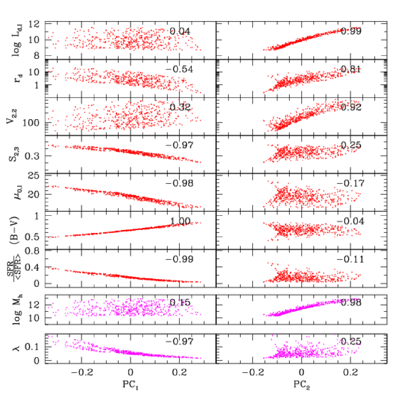
Figure 3: Correlations of observables and control parameters with the first (left column) and second (right column) principal components of Model 2.1, which has control parameters $M_{h}$ and $\lambda$. In each panel, points represent the 500 galaxies in the model realization, and numbers indicate the Spearman rank correlation coefficient with the corresponding PC. The top rows show correlations for seven of the 13 observables that enter the PCA. The bottom two rows show correlations of the control parameters, which do not enter the PCA itself but which drive the principal component structure.

Figure 2 shows only bivariate relations, and it incorporates only four of the 13 observables that we compute for each galaxy. PCA is an ideal tool for revealing the information in multi-variate correlations of large numbers of observable quantities. We apply PCA to the 13 observables of the $\sim 500$ galaxies of each of our models. Figure 3 shows the projection of seven of these observables onto the PCs recovered for Model 2.1. In addition to the luminosity, scale length, rotation speed, and $\bv$ color, we include three other quantities that have high correlations with the derived PCs: the rotation curve slope $S_{2,3}$, the I-band central surface brightness $\mu_{0,I}$, and the birth parameter $b=\,{\rm{SFR/<SFR>}}$.

Each panel shows points for each of the model galaxies, displaying correlations with the first principal component (${\rm PC}_{1}$) in the left-hand column and the second principal component (${\rm PC}_{2}$) in the right-hand column. The bottom two rows of Figure 3 show the correlations of the model control parameters, $M_{h}$ and $\lambda$, with the derived PCs. These quantities do not enter the PCA itself because they are not observable, but they are correlated with the PCs because they govern the correlations of the observables. Each panel of Figure 3 lists the Spearman rank correlation coefficient of the plotted quantity with the corresponding PC. Because these correlation coefficients depend only on rank with respect to other model galaxies, they are not affected by curvature provided that the correlation remains monotonic, and it does not matter whether we use linear or logarithmic, normalized or unnormalized variables (though these choices do matter for the computation of the PCs in the first place).

Since Model 2.1 has only two control parameters, there are, not surprisingly, only two significant principal components. ¿From Figure 3 it is evident that ${\rm PC}_{1}$ is predominantly a measure of SED shape, represented here by $\bv$ and the birth parameter, but by more observables in the PCA (see Table 2). ${\rm PC}_{1}$ is strongly anti-correlated with the central surface brightness $\mu_{0,I}$ because of the strong link between star formation history and surface density provided by the Schmidt law. Note that, because we use units of mag arcsec^-2 for $\mu_{0,I}$, high values correspond to low surface densities, and hence to slow gas consumption and blue color.

${\rm PC}_{1}$ is anti-correlated with the scale length $r_{d}$, but much less directly, since, for example, massive disks (in high $M_{h}$ halos) can have large $r_{d}$ and still have high surface densities. Because the baryon effects on the rotation curve are stronger in high surface density disks, ${\rm PC}_{1}$ is also strongly (anti-)correlated with $S_{2,3}$ and somewhat correlated with $V_{2.2}$.

${\rm PC}_{2}$ is predominantly a measure of overall scale, being tightly correlated with $L_{d,I}$ and $V_{2.2}$ and slightly less so with $r_{d}$. ${\rm PC}_{2}$ is orthogonal to ${\rm PC}_{1}$ by construction, so it is almost entirely uncorrelated with $S_{2,3}$, $\mu_{0,I}$, $\bv$, and the birth parameter, which have near perfect correlations with ${\rm PC}_{1}$. In Model 2.1, ${\rm PC}_{1}$ recovers 65% of sample variance and ${\rm PC}_{2}$ 27%. However, the relative strength of the PCs is determined largely by our choice of observables. We incorporate several different measures of SED shape into the PCA, and these are tightly coupled to each other by their similar dependence on star formation history. Thus ${\rm PC}_{1}$ accounts for much of the total variance. If we use only a single color to represent SED shape, then scale quantities make a much more important contribution to ${\rm PC}_{1}$, though they also remain correlated with ${\rm PC}_{2}$.

The bottom rows of Figure 3 demonstrate a very clean physical division between the PCs of this model. ${\rm PC}_{1}$ is driven almost entirely by variations in $\lambda$, which govern the disk surface density, and therefore the star formation history, and therefore the SED. ${\rm PC}_{2}$ is driven almost entirely by halo mass, which determines the disk luminosity and plays the dominant role in governing $V_{2.2}$ and $r_{d}$.

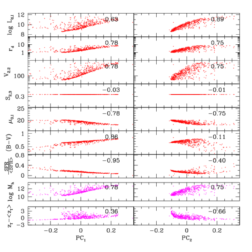
Figure 4: Same as Fig. 3, but for Model 2.2, with control parameters $M_{h}$ and $z_{f}$. Since $z_{f}$ varies systematically with halo mass, we subtract off the mean value $\langle z_{f}\rangle$ for the galaxy’s $M_{h}$ in order to isolate variations about the mean trend.

Figure 4 shows the PC correlations for Model 2.2, in which $z_{f}$ replaces $\lambda$ as the second control parameter. ${\rm PC}_{1}$ is still strongly correlated with SED quantities ($\bv$ and birth parameter in this plot), which are again tightly coupled to central surface brightness. However, with $\lambda$ variation suppressed, halo mass becomes the physical driver of surface density variations and hence the primary determinant of SED shape. Since halo mass also drives scale quantities like $V_{2.2}$, $L_{d,I}$, and $r_{d}$, these also become strong components of ${\rm PC}_{1}$, much more so than in Figure 3. Formation redshift plays a minor role in driving ${\rm PC}_{1}$, mainly as a result of galaxies with very low formation redshifts that have very blue colors. ${\rm PC}_{2}$ is again composed largely of scale quantities, but the correlations are weaker than those of Model 2.1 because the correlation of these quantities with SED properties has been absorbed into ${\rm PC}_{1}$. $M_{h}$ and $z_{f}$ are both correlated with ${\rm PC}_{2}$, with comparable strength. With our full set of observables, ${\rm PC}_{1}$ recovers more than 50% of the sample variance for this model, while ${\rm PC}_{2}$ recovers only 25%.

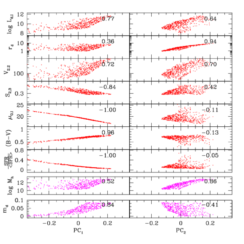
Figure 5: Same as Fig. 3, but for Model 2.3, with control parameters $M_{h}$ and $m_{d}$.

For Model 2.3 (Figure 5), ${\rm PC}_{1}$ is once again dominated by SED measures and surface brightness. The main physical driver in this case is the disk mass fraction $m_{d}$, since there are no $\lambda$ variations to induce a change in surface density, but halo mass also has a significant influence. The correlations of control parameters with ${\rm PC}_{1}$ are defined largely by “exclusion zones” — galaxies cannot attain high surface densities and red colors if they have low $m_{d}$ or low $M_{h}$, and they cannot have low surface density and blue colors if they have high $m_{d}$. Because $m_{d}$ has a direct impact on disk mass and determines the baryon contribution to the rotation curve, $L_{d,I}$, $V_{2.2}$, and $S_{2,3}$ are substantially correlated with ${\rm PC}_{1}$; the absence of red galaxies with low $M_{h}$ adds to these correlations and produces a mild correlation with $r_{d}$. ${\rm PC}_{2}$ is again correlated with scale measures, most strongly with $r_{d}$, which, in contrast to $L_{d,I}$ and $V_{2.2}$, is only minimally affected by $m_{d}$. Halo mass is the primary driver of ${\rm PC}_{2}$, though $m_{d}$ contributes, now acting in opposition to $M_{h}$ rather than in concert with it.

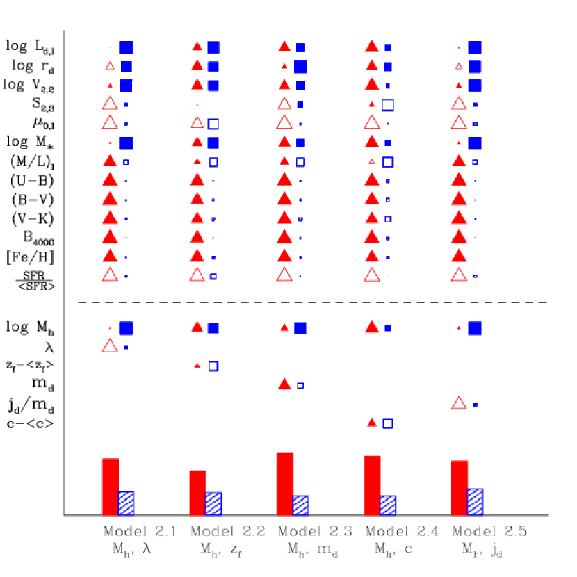
Figure 6: Summary of the PC structure of the five 2-parameter models. For each model, vertical bars at the bottom of the diagram indicate the fraction of variance accounted for by the first two PCs. In the upper part of the diagram, triangles indicate the correlation of the 13 observables with ${\rm PC}_{1}$; a filled symbol indicates positive correlation, an open symbol anti-correlation, and the linear size of the symbol is proportional to the value of the correlation coefficient. Squares show the correlation with ${\rm PC}_{2}$, in similar fashion. Below the dashed line, triangles and squares show correlations of the model control parameters with the principal components. In models with $z_{f}$ or $c$ as control parameters, correlations are computed for $z_{f}-\langle z_{f}\rangle$ or $c-\langle c\rangle$, where $\langle z_{f}\rangle$ and $\langle c\rangle$ are the mean parameter values for the galaxies’ halo mass $M_{h}$.

We would like to be able to compare the PC structure of our models directly to each other and to consider all of the observables simultaneously, and this requires a more compact representation than the one in Figures 3-5. Figure 6 is our attempt to achieve such a representation. It summarizes the results of the 2-parameter models we have examined so far, and of two additional models, 2.4 and 2.5, in which halo concentration and disk angular momentum fraction are control parameters. The bottom part of the diagram depicts the strength of the significant PCs recovered. The height of each box, solid for ${\rm PC}_{1}$ and shaded for ${\rm PC}_{2}$, is directly proportional to the amount of variance explained by each PC. The top part of the diagram, above the dashed line, displays the correlations between all 13 observables and the PCs. Triangles represent the correlations with ${\rm PC}_{1}$, and the linear size of the triangle is directly proportional to the magnitude of the Spearman correlation coefficient; filled triangles indicate positive correlation, empty triangles negative correlation. Squares represent the correlations with ${\rm PC}_{2}$, in similar fashion. Symbols below the dashed line display correlations of the model’s control parameters with the PCs. The mean values of formation redshift $z_{f}$ and concentration parameter $c$ vary with $M_{h}$, so to isolate the impact of variations in these quantities we subtract off the mean value $\langle z_{f}\rangle$ or $\langle c\rangle$ for the galaxy’s halo mass before computing correlation coefficients. Similarly, the disk’s specific angular momentum, which determines its structural properties, is proportional to $j_{d}/m_{d}$ rather than to $j_{d}$ itself, so we treat this ratio as the control parameter. As it happens, our models with varying $j_{d}/m_{d}$ have fixed $m_{d}$, and only rank values enter the Spearman correlation coefficient, so our results would be no different if we used $j_{d}$ instead, but the distinction would matter if we considered a model with independent variations in $j_{d}$ and $m_{d}$.

The main shortcoming of Figure 6 is that it summarizes correlations by a single number, the correlation coefficient. As seen in Figures 3-5, moderate or weak correlations can have a variety of detailed structures — random scatter on top of a weak or non-existent trend, definition by exclusion zones rather than a tight core, or washing out of a significant underlying correlation by relatively rare outliers. Figure 6 allows easy comparison of the overall PC structure of different models, at the price of losing this detailed information for individual cases.

The first three columns of Figure 6 summarize what we have seen in Figures 3-5. In each model, ${\rm PC}_{1}$ is largely a measure of SED shape; newly plotted observables $(U-B)$, $(V-K)$, and $B_{4000}$ are also strongly correlated with ${\rm PC}_{1}$. The SED shape is always strongly correlated with surface brightness because of the Schmidt-law connection between star formation rate and surface density. (The sign of this correlation is negative because of the mag arcsec^-2 units.) ${\rm PC}_{2}$ is correlated mainly with scale variables like $L_{d,I}$, $r_{d}$ and $V_{2.2}$. However, the physical parameters determining ${\rm PC}_{1}$ are different in each case: $\lambda$ in Model 2.1, $M_{h}$ in Model 2.2, and a combination of $m_{d}$ and $M_{h}$ in Model 2.3, with $m_{d}$ being dominant.

Differences in the governing parameters lead to some important differences in PCs. In Model 2.1, we see the dominance of the broad $\lambda$ distribution in determining the surface density. This leads to anti-correlation of $S_{2,3}$ and $r_{d}$ with ${\rm PC}_{1}$ and essentially no correlation between $L_{d,I}$ and ${\rm PC}_{1}$. In Model 2.2, the greater importance of $M_{h}$ in setting the surface density forces scale quantities to move partly into ${\rm PC}_{1}$, and the sign of the correlation between $r_{d}$ and ${\rm PC}_{1}$ reverses. In Model 2.3, $m_{d}$ variations link $L_{d,I}$ to surface density and thus to the shape of the SED. However, $r_{d}$ remains in ${\rm PC}_{2}$ because it is determined mainly by $M_{h}$ (and by $\lambda$, which is fixed). $V_{2.2}$ has similar correlations with ${\rm PC}_{1}$ in all three models, but for somewhat different reasons: in 2.1 and 2.3 because $\lambda$ or $m_{d}$ determines the surface density and the baryon contribution to $V_{2.2}$, in 2.2 because $M_{h}$ determines the surface density and the halo contribution to $V_{2.2}$. The rotation curve slope is strongly anti-correlated with ${\rm PC}_{1}$ in the models where the baryon contribution to the rotation curve varies substantially, but it is uncorrelated with either PC (and hardly variable at all) in Model 2.2, where the baryon contribution is constant.

The last two columns of Figure 6 show results for two more 2-parameter models. In Model 2.4, only $M_{h}$ and the concentration parameter $c$ vary. Most observables now have a stronger correlation with ${\rm PC}_{1}$ than with ${\rm PC}_{2}$, the only exceptions being the rotation curve slope and the stellar mass-to-light ratio. ${\rm PC}_{1}$ is driven primarily by halo mass, with a small contribution from concentration. ${\rm PC}_{2}$ depends on the opposite combination of mass and concentration (anti-correlated instead of correlated), and concentration dominates. Less concentrated halos host galaxies with flatter rotation curves, slightly larger disks, and (as a consequence of slower star formation rates) lower $(M/L)_{I}$.

Model 2.5 has all parameters fixed except $M_{h}$ and $j_{d}$, the ratio of disk to halo angular momentum. In many ways, the physics of this model is similar to that of Model 2.1, since only halo mass and disk angular momentum vary. The distribution of angular momentum is narrower in this model — in particular, there are no very large values because the maximum angular momentum comes for $\lambda=0.05$, $j_{d}=1$. However, this difference in distributions does not have a large effect on the PC structure, and the correlations between the observables and the PCs are nearly identical to those found for Model 2.1.

4.2 The Baseline Model

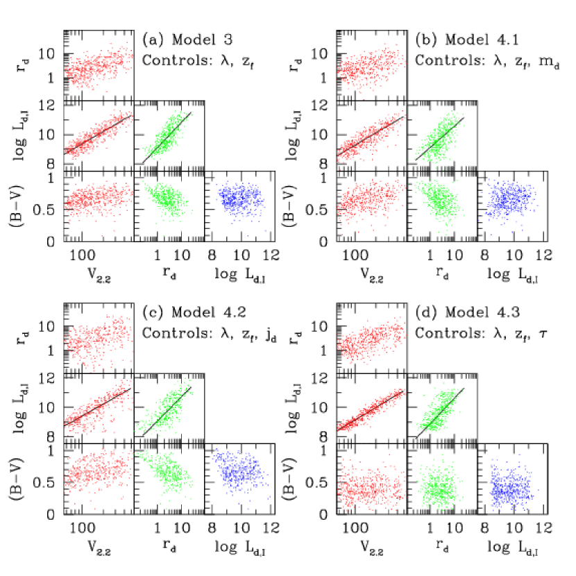
Figure 7: Bivariate correlations for models with three or four control parameters, in the same format as Fig. 2. Note that, in addition to the parameters listed, $M_{h}$ is a control parameter in every model. Model 3 is the “baseline model,” with control parameters $M_{h}$, $\lambda$, and $z_{f}$. Models 4.1 and 4.2 extend the baseline model by adding $m_{d}$ or $j_{d}$ as an additional control parameter. Model 4.3 decouples the star formation rate from the gas surface density, adding a randomly chosen exponential decay timescale $\tau$ as a control parameter.

A realistic model of galaxy formation should include, at a minimum, the expected variations in halo mass, spin parameter, and halo formation redshift. We define Model 3, with these three control parameters, to be our “baseline model.” Figure 7a shows bivariate correlations for this model. The observed scatter is now determined by the variation (at given mass) of $\lambda$ and $z_{f}$. The correlations and scatter in Figure 7a are similar to those of Model 2.1 shown in Figure 2b, indicating that $z_{f}$ variations (suppressed in Model 2.1) have only small impact relative to $M_{h}$ and $\lambda$. There are clear correlations among $r_{d}$, $L_{d,I}$ and $V_{2.2}$, with the scatter from $\lambda$ variations especially evident in the R-V relation. Variations in formation redshift add scatter to the correlations of color with other parameters, but they do not erase them or change their sign, confirming the dominant role of $\lambda$ in determining the star formation history through the surface density.

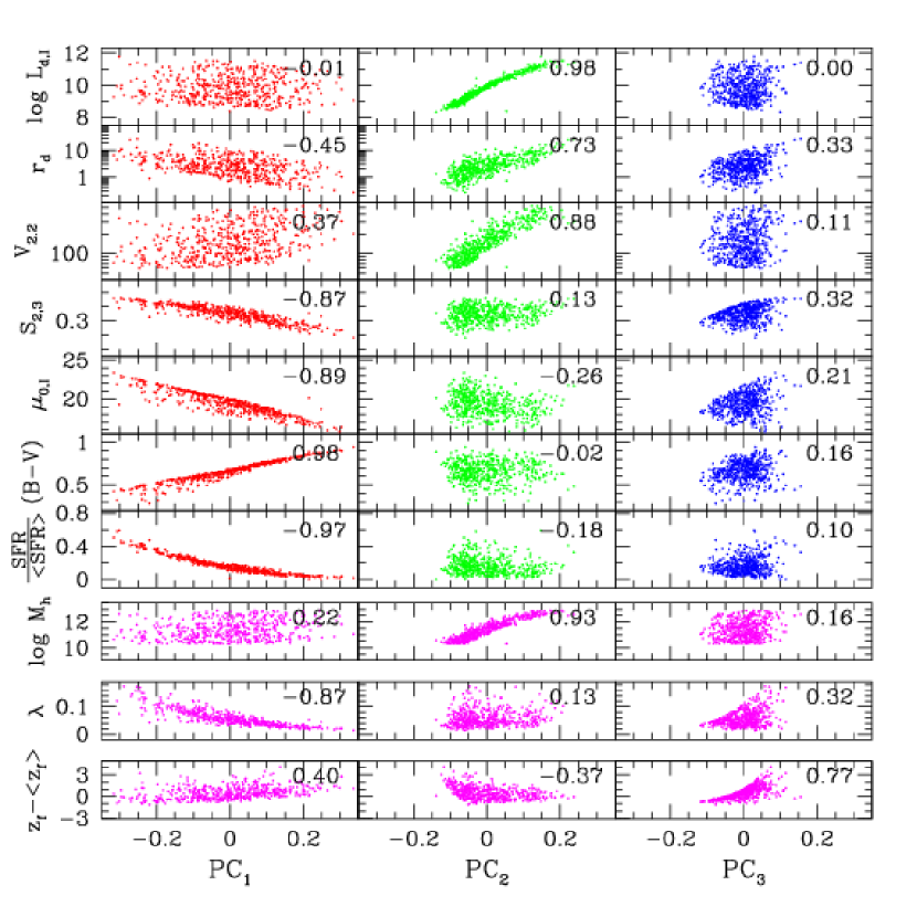
Figure 8: Correlations of observables (top) and control parameters (bottom) with the three principal components of the baseline model, Model 3, which has control parameters $M_{h}$, $\lambda$, and $z_{f}$. Format is the same as Fig. 3.

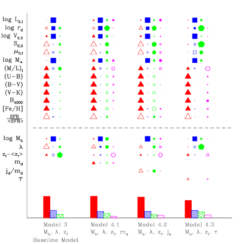
Figure 10: Principal component structure of the models with three or four control parameters, in the same format as Fig. 6. Correlations with the $n$th PC are represented by symbols with $n+2$ sides, filled for positive correlation, open for anti-correlation, with linear size proportional to the correlation coefficient. The leftmost column encapsulates the predictions of the “standard” theory of disk galaxy formation, our baseline model, in which $M_{h}$, $\lambda$, and $z_{f}$ determine disk structural parameters and the Schmidt law determines the star formation history given these parameters. Other columns show results for models in which variations in other physical processes contribute to variations in galaxy properties.

PCs for the baseline model are illustrated in Figure 8 and in the first column of Figure 10. Results are again reminiscent of those for Model 2.1 (see Figure 3 and the first column of Figure 6), but the addition of $z_{f}$ as a control parameter adds complexity. The first PC is dominated as usual by SED quantities, which are strongly anti-correlated with $\mu_{0,I}$, weakly correlated with $V_{2.2}$, moderately anti-correlated with $r_{d}$, and entirely uncorrelated with $L_{d,I}$. The physical parameter driving ${\rm PC}_{1}$ is $\lambda$, through its impact on surface density, though there are small contributions from $z_{f}$ and $M_{h}$. The greater importance of disk self-gravity and adiabatic contraction in low-spin systems couples $S_{2,3}$ into ${\rm PC}_{1}$.

The second PC is again comprised mainly of scale quantities $L_{d,I}$, $r_{d}$ and $V_{2.2}$. As in Model 2.1, ${\rm PC}_{2}$ is driven mainly by $M_{h}$, but now there is a slight contribution from $z_{f}$. The addition of a third control parameter leads to the appearance of a third, relatively weak PC, involving the stellar mass-to-light ratio, the rotation curve slope, the disk scale length, and the central surface brightness. ${\rm PC}_{3}$ is driven mainly by $z_{f}$ variations, and to successively smaller degrees by $\lambda$ and $M_{h}$, but it does not have an obvious simple interpretation. It seems to arise mainly because $z_{f}$ and $\lambda$ compete in their contributions to ${\rm PC}_{1}$, and a different combination of them (correlated instead of anti-correlated) causes orthogonal variation in other observables. We will discuss the PC structure of the baseline model further in Section 4.4.

Numerical and analytic studies of halo formation predict significant variations in concentration, so one could argue that $c$ variations should be included in our baseline model. However, we have already seen in Figure 6 that the influence of $c$ on PC structure is relatively small. We have investigated a case in which we add $c$ variations to the baseline model, and the effects are minor as expected. The first two principal components are entirely unchanged, but ${\rm PC}_{3}$ changes to some degree, splitting into two weak PCs that involve similar observables in somewhat different combinations. Halo concentration is not a major driver in any of these principal components. Because of its relatively small impact, we have opted for simplicity and eliminated $c$ variations in our baseline model and the extensions discussed below.

4.3 Extended Models

We can now ask what happens if we add new physical ingredients to the baseline model, represented by additional control parameters. Parameter correlations for three such extended models are illustrated in Figures 7b-d. Figure 7b shows Model 4.1, in which $m_{d}$ varies in addition to $M_{h}$, $\lambda$, and $z_{f}$. This additional variation causes remarkably little change in the correlations, relative to the baseline model shown in Figure 7a. The scatterplots display a somewhat increased number of outliers, but the cores of the correlations do not change. This small impact of $m_{d}$ variations could be anticipated on the basis of Figure 2d.

Figure 7c shows a model with $m_{d}$ fixed at $0.5f_{b}$ but $j_{d}/m_{d}$ varying uniformly in the range $(0,1]$. Here the scatter in correlations is considerably larger than in the baseline model because of the larger range in disk angular momentum. Nevertheless, the mean correlations are not fundamentally different from those of Model 3.

Figure 7d illustrates a more radical change to the baseline model. Instead of the Schmidt law, we use an exponentially decaying SFR beginning at $z_{f}$ with decay timescale $\tau$ chosen from a uniform distribution $[1,9]$ Gyr, as described in §2.4. This model specifically breaks the link between the star formation history and the structural quantities that determine surface density. As a result, color is uncorrelated with $V_{2.2}$, $r_{d}$ and $L_{d,I}$.

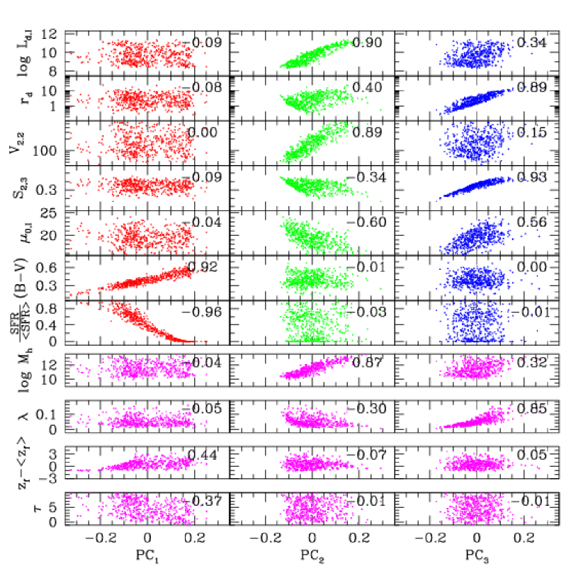
Figure 9: Same as Fig. 8, but for Model 4.3, which decouples star formation from surface density and adds the exponential star formation timescale $\tau$ as a control parameter.

Figure 9 illustrates the PCs of this model. SED quantities still dominate the first component, and in contrast to the baseline model (Figure 8) they are no longer correlated at all with $\mu_{0,I}$, $r_{d}$, or $V_{2.2}$. Furthermore, ${\rm PC}_{1}$ is now determined by a combination of $z_{f}$ and $\tau$, rather than the combination of $z_{f}$ and $\lambda$ that drives ${\rm PC}_{1}$ in the baseline model. Also in contrast to the baseline model, Model 4.3 has second and third PCs of nearly equal strength (see the fourth column of Figure 10), both of them composed mainly of scale quantities and surface brightness, but in different combinations. ${\rm PC}_{2}$ is largest when $M_{h}$ is large and $\lambda$ is small; this combination produces disks with high luminosity, high circular velocity, and high surface brightness (low $\mu_{0,I}$), but the competing effects on scale length leave $r_{d}$ only moderately correlated with ${\rm PC}_{2}$. ${\rm PC}_{3}$ is largest when $M_{h}$ and $\lambda$ are both large; this combination produces disks with large scale length and (less consistently) low surface brightness and high luminosity. However, the competing effects on halo and disk contributions to the rotation curve leave $V_{2.2}$ almost uncorrelated with ${\rm PC}_{3}$. Decoupling star formation from surface density allows the correlated and anti-correlated combinations of $M_{h}$ and $\lambda$ to drive separate principal components of comparable strength, with $M_{h}$ playing the stronger role in one (${\rm PC}_{2}$) and $\lambda$ in the other (${\rm PC}_{3}$). In the baseline model, by contrast, the strong coupling of $\lambda$ into the SED principal component leaves mass as the sole driver of ${\rm PC}_{2}$. In terms of the observables, models with a Schmidt law prescription must have surface brightness strongly correlated with SED shape, and it is only abandoning this prescription that allows correlated and anti-correlated trends of surface brightness with other structural quantities to appear as separate principal components.

4.4 Summary

Figure 10 summarizes our results for the baseline model and for the extended models discussed in § 4.3. The format is similar to that of Figure 6, but since these models have three or four control parameters, there are three or four significant PCs.

The leftmost column encapsulates the predictions of the “standard” theory of disk galaxy formation (our baseline model), in which $M_{h}$, $\lambda$, and $z_{f}$ determine disk structural parameters and the Schmidt law determines the star formation history given these parameters. The first PC is basically a measure of SED shape, strongly correlated with surface brightness because of the Schmidt law. ${\rm PC}_{1}$ is also correlated with $V_{2.2}$, and with $S_{2,3}$, because of the baryonic influence on the rotation curve. The second PC consists mainly of scale quantities such as $L_{d,I}$, $r_{d}$, and $V_{2.2}$. Physically, the first PC is driven mainly by $\lambda$, the second mainly by $M_{h}$. Variations in $z_{f}$ drive the relatively weak third PC, which has correlated contributions from $r_{d}$, $S_{2,3}$, $\mu_{0,I}$, and $(M/L)_{I}$.

One interesting if somewhat disappointing result of our analysis is that extending the baseline model by adding stochastic variations in $m_{d}$ makes little difference to the predicted PC structure (Model 4.1, 2nd column). The first two PCs of Model 4.1 are nearly identical to those of Model 3, though in this case ${\rm PC}_{1}$ is driven by a combination of $m_{d}$ and $\lambda$ instead of by $\lambda$ alone, and it picks up small contributions from $L_{d,I}$ and $M_{\star}$ as a result. The third PC is noticeably different, having stronger correlations (especially with $r_{d}$ and $S_{2,3}$) and a non-negligible contribution from SED observables. The addition of $m_{d}$ as a variable that influences surface density allows a correlated contribution of $M_{h}$ and $\lambda$ to drive larger variations in $r_{d}$, which are correlated in turn with $S_{2,3}$ because extended disks have less dynamical impact. The fourth PC, driven by $z_{f}$ variations, is very weak; this is the only case where we plot a PC with variance less than our statistically motivated threshold of 0.7 (see §3).

As discussed in §4.1 with regard to Model 2.3, $m_{d}$ variations have less impact on the scatter of the L-V relation than one might expect because disk gravity effects tend to shift points parallel to the L-V locus as $m_{d}$ changes. The mean value of $m_{d}$ should have a noticeable effect on the zero points of some relations, such as L-R, and on the relative velocity scales inferred at fixed luminosity from rotation curves (which probe the regime where disk gravity is important) and from weak lensing measurements (which probe larger scales). However, the effect of scatter in $m_{d}$ is harder to discern. The differences in ${\rm PC}_{3}$ between Models 3 and 4.1 are probably large enough to be observable, but it is less clear that they are larger than uncertainties associated with the approximations of our modeling. At the least, comparison of Models 3 and 4.1 implies that agreement between observed correlations of galaxy properties and predictions of the baseline model, if found in the data, should not be taken as immediate evidence that $m_{d}$ is constant from halo to halo. Measurements of rotation velocity at somewhat larger radii, $3-5r_{d}$, could be helpful in revealing effects of $m_{d}$ scatter, since they are less influenced by the gravity of the disk (Shen, Mo, & Shu 2001).

Adding variations in angular momentum loss to the baseline model also has little effect on the first two principal components (Model 4.2, 3rd column). It is now a combination of $\lambda$ and $j_{d}$ that drives ${\rm PC}_{1}$, and $M_{h}$ still drives ${\rm PC}_{2}$. The broader angular momentum distribution increases the scatter in bivariate relations (see Figure 7), but the overall correlation structure is much the same. The third PC, on the other hand, resembles that of Model 4.1 rather than Model 3, and it is driven again by a correlated contribution of halo mass and disk angular momentum. Formation redshift provides the main contribution to the fourth PC, which is similar to that of Model 4.1. However, ${\rm PC}_{4}$ has no strong correlation with any of the observables, and its statistical significance is marginal.

Breaking the Schmidt-law link between star formation and surface density makes an important difference to the PC structure, leading to a clean separation between SED quantities and structural quantities (Model 4.3, 4th column). Central surface brightness and rotation curve slope vanish from ${\rm PC}_{1}$, where they had a strong presence in all of our previous models. The weak contributions of $r_{d}$ and $V_{2.2}$ also disappear. The coherent SED variations that comprise ${\rm PC}_{1}$ are driven mainly by formation redshift and the exponential decay timescale. There are now two PCs comprised of scale quantities, both of nearly equal strength, driven by $M_{h}$ and $\lambda$ in two different combinations (correlated and anti-correlated). The first of these contains correlated contributions of $L_{d,I}$ and $V_{2.2}$ and the anti-correlated contribution of $\mu_{0,I}$, but it has only a moderate contribution from $r_{d}$. The second represents correlation of $r_{d}$, $S_{2,3}$ and $\mu_{0,I}$, with moderate contribution from $L_{d,I}$. Finally, $PC_{4}$, associated with $z_{f}$ and $\tau$, accounts for some of the variance in $(M/L)_{I}$.

5 Conclusions and Outlook

The techniques describe in §2 and §3 allow us to predict the principal component structure of the disk galaxy population, given different assumptions about the control parameters that govern the origin of galaxies’ observable properties (see Tables 1 and 3). By examining the correlation of the principal components with the input parameters, we also learn what physical processes drive these components in different galaxy formation models. Our list of observables (Table 2) includes three broad band colors, the 4000Å break, and the birth parameter $b=\,{\rm{SFR/<SFR>}}$, and these quantities are highly correlated with each other because they are all determined by the galaxy’s star formation history. As a result, these SED parameters dominate the first principal component, ${\rm PC}_{1}$, in all of our models. ${\rm PC}_{2}$ is usually a measure of overall scale, with strong contributions from luminosity, circular velocity, disk scale length, and stellar mass.

Distinctions among our models appear in the apportioning of these scale observables and two other structural quantities, the central surface brightness and rotation curve slope, among ${\rm PC}_{1}$ and ${\rm PC}_{2}$, and in some cases ${\rm PC}_{3}$. These apportionments depend in turn on the governing physics of the model. In all models that have a Schmidt-law prescription for star formation, the central surface brightness is strongly correlated with ${\rm PC}_{1}$ because of the strong coupling between star formation history and surface density. In models where angular momentum and/or disk mass fraction control the surface density, high surface brightness disks also have large baryon contributions to the rotation curve, producing a strong coupling to $S_{2,3}$. Our baseline model has $M_{h}$, $\lambda$, and $z_{f}$ as control parameters, and because the log-normal distribution of $\lambda$ is very broad, it dominates the distribution of disk surface densities and drives ${\rm PC}_{1}$. Halo mass drives ${\rm PC}_{2}$, and formation redshift drives a weak third component. When $m_{d}$ or $j_{d}$ become additional control parameters, they share direction of ${\rm PC}_{1}$ with $\lambda$, and this allows a correlated combination of halo mass and angular momentum to produce a new third PC that has substantial correlations with $r_{d}$ and $S_{2,3}$. The most significant change to the PC structure comes from replacing the Schmidt law by an exponentially declining star formation prescription with decay timescale chosen independently of surface density. Surface brightness and $S_{2,3}$ disappear from the first principal component, and correlated and anti-correlated combinations of $M_{h}$ and $\lambda$ drive two different PCs of nearly equal strength, each involving a combination of structural quantities. Thus, PCA of the observed disk galaxy population can distinguish among different models for the origin of galaxy properties.

There are numerous ways to improve or extend our models of disk galaxy formation and thus provide a more comprehensive framework for understanding the implications of PCA. One of the most obvious ingredients missing from our calculations is a model of dust extinction and scattering, which can have important effects on luminosities, colors, and mass-to-light ratios. Since the impact of dust is highly dependent on inclination, one would need to include inclination or axis ratio as an additional observable in models that incorporate dust. Alternatively, one can determine empirical corrections for internal extinction and correct the data to values for face-on disks. Given the complexities and uncertainties of realistic dust modeling (see, e.g., Wood & Jones 1997; Silva et al. 2001), this empirical correction approach, already commonly used in Tully-Fisher analyses (see Tully & Fouque 1985), may be preferable to adding dust to the models.

Since the star formation prescription plays such a fundamental role in governing the PC structure of our models, it would be interesting to explore alternatives to the Schmidt law that are not as extreme as our exponential decay model, which decouples star formation from structural quantities completely. The assumption that star formation continues until the effective local value of the Toomre (1964) instability parameter $Q$ exceeds some threshold (see Gunn 1981, 1983, 1987) is one example of such an alternative, and the role of disk self-gravity in determining $Q$ might lead to a significantly different correlation between SED and structural quantities in ${\rm PC}_{1}$. Our models also subsume all of the complex physics of gas cooling and feedback into the single parameter $m_{d}$. If these processes are sufficiently self-regulating that $m_{d}$ is nearly constant, or if variations of $m_{d}$ are truly stochastic, then our simple description may well be adequate to our purpose. However, one could imagine that a more detailed model of cooling and feedback would connect variations in disk mass fraction to variations in star formation history or galaxy structure, and that these connections might in turn alter the structure of principal components.

Fundamental to our models is the assumption that disk sizes are determined by the combination of halo virial radii with angular momentum parameters ($\lambda$ and in some cases $j_{d}$) that vary independently of other model inputs. The influence of angular momentum on the galaxy’s stellar population is “one way,” with disk scale length determining the star formation rate through the Schmidt law. This assumption seems fairly plausible even if the process of disk assembly is messier than the one envisioned in our adopted formalism, but it is not incontrovertible. While the theoretically predicted distribution of $\lambda$ yields rough agreement with the observed distribution of disk sizes (Syer, Mao, & Mo 1999; de Jong & Lacey 2000), the detailed distribution of specific angular momentum within halos would not, if preserved by the collapsing baryons, yield exponential disks (Ryden 1988; Bullock et al. 2001a; van den Bosch 2001). An alternative explanation for exponential stellar disks is viscous redistribution of disk material on the same timescale as star formation (Lin & Pringle 1987; Slyz et al. 2001). A model incorporating this kind of “back reaction” of star formation on scale length might make distinctive predictions for PC structure. The dynamical interactions between baryons and the dark halo could well be more complicated than the adiabatic contraction model we have used, for example because of resonant interactions with rotating bars (Hernquist & Weinberg 1992; Weinberg & Katz 2001), and such interactions might also alter PCA predictions in distinctive ways.

The most important and challenging direction for extending our models is to incorporate bulge formation and transformation among morphological types. In contrast to disk formation, there is no “standard model” of bulge formation, though the idea that mergers transform stellar disks into spheroids is the one that has been most widely explored in semi-analytic models (Baugh, Cole, & Frenk 1996; Kauffmann 1996; Somerville & Primack 1999). Alternative ideas include secular bulge formation via bar instability (Raha et al. 1991; van den Bosch 2001), association of rapid early star formation with spheroids and slower subsequent star formation with disks (Eggen, Lynden-Bell, & Sandage 1962), and morphological transformation in groups and clusters caused by weak dynamical perturbations (Moore, Lake, & Katz 1998) or interactions with intergalactic gas (Gunn & Gott 1972). Galaxy formation models that incorporate these processes could predict the PC structure of the full galaxy population instead of the isolated disk systems that we have considered, and they would show whether PCA can diagnose the relative importance of different mechanisms for morphological transformation. The calculational approach needed for such models is more complicated than the one we have employed in this paper, requiring halo and galaxy merger trees. One fortunate by-product of such an approach would be descriptions of the local environment — field, group, cluster — of each model galaxy. These environmental descriptions could be incorporated as additional observables in PCA, and they would likely add considerable power for diagnosing the origin of morphological properties.

The advantages of semi-analytic models for PCA predictions are computational speed, the relatively transparent links between input parameters and output observables, and the ease with which one can vary model assumptions and examine their impact on PC structure. However, hydrodynamic simulations incorporate more realistic descriptions of some of the essential physical processes — gravitational collapse, gas dynamics and cooling, galaxy mergers within common halos — and they are approaching the point where they could usefully be analyzed with the same multi-variate techniques employed here. High resolution simulations of individual galaxies (e.g., Navarro & Steinmetz 2000) can predict many of the quantities that we have used in our analysis, and improvements in computer hardware and algorithms should eventually allow creation of the kinds of ensembles that would be needed for PCA. An intermediate option is to use somewhat lower resolution simulations of large volumes (e.g., Pearce et al. 1999; Murali et al. 2001; Nagamine et al. 2001; Yoshikawa et al. 2001) to predict the baryonic masses, assembly histories, environments, and total angular momenta of galaxies, and to supplement these with models of the sub-resolution physics that translates these global quantities into direct observables. The combination of numerical and semi-analytic approaches could be fruitful, with numerical simulations calibrating the semi-analytic calculations for matched assumptions and semi-analytic calculations illustrating how changes to the input assumptions might alter the numerical predictions.

The recent convergence on a well defined cosmological model has solidified the ground beneath a basic picture of galaxy formation that has emerged over the last 25 years: galaxies form after gas collapses and dissipates within collisionless dark matter halos, which form by gravitational instability from initial conditions that are not far from those of the $\Lambda$CDM scenario. However, there are still many competing ideas for the origin of galaxy luminosities, sizes, colors, morphologies, and dynamical properties, and even the leading ideas have not been tested extensively against observations. As illustrated in this paper, any theory that predicts these observable quantities also predicts the correlations among them, which can be well summarized using the techniques of Principal Component Analysis. Comparison of these predictions to PCA results from the SDSS and other large surveys should take us a long way towards understanding how the observable properties of galaxies are connected to the governing physics of galaxy formation.

Appendix

Appendix A Chemical Enrichment

We compute the chemical enrichment in each model galaxy by solving the following integro-differential equation:

$$M_{g}\frac{dZ}{dt}=E_{Z_{new}}(t)+E_{Z_{old}}(t)-Z(t)[E(t)+F(t)]\ ,$$ (A1)

where $M_{g}$ is the available gas content, $Z(t)$ is the metal abundance by mass, $F$ is the infall rate of pristine gas, and $E$ is the ejection rate of matter by evolved stars. The choice of an infall rate is more problematic than the choice of SFR, since both theoretical and observational constraints are much less obvious. Here we assume that pristine gas falls onto the disk at a rate exponentially decreasing with time. Stars are formed at a rate proportional to the surface gas density (Lacey & Fall 1983). In order to reproduce the observed abundance gradients, Lacey & Fall (1983) suggested that the infall timescale should be an increasing function of galactocentric radius. We assume an exponential form of the infall time scale dependence $\tau(r)=\tau_{0}\exp(r/r_{d})$, where $r_{d}$ is the disk scale length. The characteristic timescale $\tau_{0}$ depends on the total mass of the disk through the relation $\tau_{0}=\tau_{\odot}(M_{d}/M_{d,MW})^{-1/2}$, where the subscript MW refers to the Milky Way and $\tau_{\odot}=4\;$Gyr is the collapse timescale for the solar neighborhood (Molla, Hardy, & Beauchamp 1999; Ferrini et al. 1994). We further assume the infalling gas to be at primordial metallicity.

The term representing the gas ejection rate in equation (A1) can be defined as a simple function of SFR, IMF, metallicity, and mass:

$$E(t)=\int^{m_{u}}_{m_{(m,Z_{\star})}}mp(m,Z_{\star})\phi(m)\psi(t-\tau(m,Z_{\star}))dm\ .$$ (A2)

Here $p(m,Z_{\star})=[m-m_{\rm rem}(m,Z_{\star})]/m$ is the returned mass fraction of stars of mass $m$ and remnant mass $m_{\rm rem}$, $\psi(t-\tau(m,Z_{\star}))$ is the SFR by number at the time a star of initial mass $m$ and metallicity $Z_{\star}$ was formed, $\tau(m,Z_{\star})$ is the lifetime of a star of initial mass $m$ born with metallicity $Z_{\star}$, and $m_{t}(m,Z_{\star})$ is the current turnoff mass.

The total ejection rate of metals can be expressed as the sum of two terms: the first term takes into account the newly synthesized and ejected metals, the second accounts for the rate of ejection of unprocessed metals, i.e. those that originate from the material out of which the star was formed. In detail:

$$E_{Z_{new}}(t) = \int^{m_{u}}_{m_{(t,Z_{\star})}}mp_{z}(m,Z_{\star})\phi(m)\psi(t-\tau(m,Z_{\star}))dm$$ (A3)

$$E_{Z_{old}}(t) = \int^{m_{u}}_{m_{(t,Z_{\star})}}mp(m,Z_{\star})Z(t-\tau(m,Z_{\star}))\phi(m)\psi(t-\tau(m,Z_{\star}))dm\ ,$$ (A4)

where $p_{z}(m,Z_{\star})$ is the heavy element integrated stellar yield, which is defined relative to the initial metal abundance of the star, and $Z_{\star}=Z(t-\tau(m,Z_{\star}))$ is the initial metal abundance of stars that evolve off the red giant branch at age $t$. From equations (A1), (A2), and (A3), it is evident that the present metal abundance is very sensitive to the solution of the metallicity equation in the past.

Direct computation of $E(t)$ using equation (A2) cannot be achieved without detailed knowledge of $Z(t)$, unless a numerical (iterative) procedure is used. Recently, however, van den Hoek (1997) showed that if one assumes that at any time during the galaxy evolution $Z(t-\tau(m,Z_{\star}))\leq Z(t)$, then $E_{Z_{old}}(t)\leq Z(t)E(t)$. If we now define $E_{Z_{old}}(t)-Z(t)E(t)\equiv G(t)Z(t)$, equation (A1), which describes the chemical enrichment, can be written as (van den Hoek 1997):

$$\frac{dZ}{dt} = \frac{1}{M_{g}(t)}\left\{-Z(t)[G(t)+F(t)]+E_{Z_{new}}(t)\right\}$$ (A5)

$$= -Z(t)P(t)+Q(t)~{},$$ (A6)

where

$$P(t) = \frac{1}{M_{g}(t)}\left[G(t)+F(t)\right]$$ (A7)

$$Q(t) = \frac{1}{M_{g}(t)}E_{Z_{new}}(t)~{}.$$ (A8)

Finally, by integrating over time, we obtain the general solution for the gas metallicity at time $t$:

$$Z(t)=e^{-\int^{t}P(\tau)\,d\tau}\times\left[Z(t=0)+\int^{t}\frac{Q(\tau)}{e^{-\int^{t}P(\tau^{\prime})\,d\tau^{\prime}}}\,d\tau\right]~{}.$$ (A9)

All integrals are computed taking explicitly into account the finite lifetime $\tau_{m}$ of a star of mass $m$ and the metal abundance $Z_{\star}$ at its formation time $(t-\tau_{m})$. We used metallicity dependent stellar lifetimes and yields from the chemically consistent models of Marigo (1998), for stellar masses $m<6M_{\odot}$, and of Portinari, Chiosi, & Bressan (1998), for stellar masses up to $125M_{\odot}$. Both these authors give tables of lifetimes and yields as a function of mass for five discrete metallicities: $Z=0.0004$, $Z=0.004$, $Z=0.008$, $Z=0.02$, $Z=0.05$. We then linearly interpolate in $m$ and $Z$ where necessary. We further assume that each star expels its ejecta all at once at the end of its lifetime, and that the ejected material is immediately mixed in the ISM, which remains always homogeneous. It is worth mentioning that this “instantaneous mixing approximation” is only suitable to reproduce average trends observed in the age–metallicity relation and abundance ratios (Portinari, Chiosi, & Bressan 1998; van den Hoek & de Jong 1997).

Table 1: Theoretical parameters that define a galaxy.

Inputs
Halo Mass: $M_{h}$
Halo Concentration Parameter: $c$
Halo Spin Parameter: $\lambda$
Halo Formation Redshift: $z_{f}$
Disk Mass Fraction: $m_{d}=M_{d}/M_{h}$
Disk Angular Momentum Fraction: $j_{d}=J_{d}/J_{h}$
E-folding time of exponentially decaying SFR†: $\tau$

Table 2: Observable Outputs^†

Outputs
I-band Luminosity (log): $\log L_{d,I}$ $[L_{\odot}]$
Disk Scale Length (log): $\log r_{d}$ [kpc]
Rotational Velocity at Disk’s Maximum (log): $\log V_{2.2}$ $[\,{\rm{km\,s^{-1}}}]$
Rotation Curve Slope: $S_{2,3}$
I-band Central Surface Brightness: $\mu_{0,I}$ [mag arcsec-2]
Stellar Mass (log): $\log M_{\star}$ $[M_{\odot}]$
I-band Stellar Mass-to-Light Ratio: $M_{\star}/L_{I}$ $[M_{\odot}/L_{\odot}]$
Broad-band Colors: $(U-B)$, $(B-V)$, $(V-K)$
Amplitude of 4000Å break: $B_{4000}$
Mean Metallicity: $[{\rm Fe/H}]$
Birth Parameter: $b$ = $\,{\rm{SFR/<SFR>}}$

Table 3: Model Parameters^†

Control Parameters	$z_{f}$	$m_{d}/f_{b}$	$j_{d}/m_{d}$	$\lambda$	c	SFR
Model 1: $M_{h}$	$\bar{z}_{f}(M_{h})$	0.5	1	0.05	${\bar{c}}(M_{h})$	Kennicutt
Model 2.1: $M_{h}$, $\lambda$	$\bar{z}_{f}(M_{h})$	0.5	1	-1	${\bar{c}}(M_{h})$	Kennicutt
Model 2.2: $M_{h}$, $z_{f}$	-1	0.5	1	0.05	${\bar{c}}(M_{h})$	Kennicutt
Model 2.3: $M_{h}$, $m_{d}$	$\bar{z}_{f}(M_{h})$	-1	1	0.05	${\bar{c}}(M_{h})$	Kennicutt
Model 2.4: $M_{h}$, $c$	$\bar{z}_{f}(M_{h})$	0.5	1	0.05	-1	Kennicutt
Model 2.5: $M_{h}$, $j_{d}$	$\bar{z}_{f}(M_{h})$	0.5	-1	0.05	${\bar{c}}(M_{h})$	Kennicutt
Model 3: $M_{h}$, $\lambda$, $z_{f}$	-1	0.5	1	-1	${\bar{c}}(M_{h})$	Kennicutt
Model 4.1: $M_{h}$, $\lambda$, $z_{f}$, $m_{d}$	-1	-1	1	-1	${\bar{c}}(M_{h})$	Kennicutt
Model 4.2: $M_{h}$, $\lambda$, $z_{f}$, $j_{d}$	-1	0.5	-1	-1	${\bar{c}}(M_{h})$	Kennicutt
Model 4.3: $M_{h}$, $\lambda$, $z_{f}$, $\tau$	-1	0.5	1	-1	${\bar{c}}(M_{h})$	Exponential

References

- (1)
- Avila-Reese & Firmani (1998) Avila-Reese, V., & Firmani, C., 1998, ApJ, 505, 37
- Barnes & Efstathiou (1987) Barnes, J. E., & Efstathiou, G. 1987, ApJ, 319, 575
- Baugh, Cole, & Frenk (1996) Baugh, C. M., Cole, S., & Frenk, C. S., 1996, MNRAS, 283, 1361
- Blanton et al. (2001) Blanton, M. R. et al. 2001, AJ, 121, 2358
- Blumenthal et al. (1986) Blumenthal, G. R., Faber, S. M., Flores, R., & Primack, J. R. 1986, ApJ, 301, 27
- Bond et al. (1991) Bond, J. R., Cole, S., Efstathiou, G., & Kaiser, N. 1991, ApJ, 379, 440
- Bower (1991) Bower, R. 1991, MNRAS, 248, 332
- Bruzual & Charlot (1993) Bruzual, G., & Charlot, S. 1993, ApJ, 405, 538
- Bruzual & Charlot (2001) Bruzual, G., & Charlot, S. 2001, in preparation
- Bullock et al. (2001a) Bullock, J.S., Dekel, A., Kolatt, T.S., Kravtsov, A., Klypin, A. A., Porciani, C., & Primack, J.R., 2001a, ApJ, 555, 240
- Bullock et al. (2001b) Bullock, J. S., Kolatt, S. T., Sigad, Y., Somerville, R. S., Kravtsov, A. V., Klypin, A., Primack, J. R., & Dekel, A. 2001b, MNRAS, 321, 559
- Burles, Nollett & Turner (2001) Burles S., Nollett K. M & Turner S. M. 2001, ApJ, 552, 1
- Catelan & Theuns (1996a) Catelan, P., & Theuns, T. 1996a, MNRAS, 282, 436
- Catelan & Theuns (1996b) Catelan, P., & Theuns, T. 1996b, MNRAS, 282, 455
- Charlot & Bruzual (1991) Charlot, S., & Bruzual, A. G. 1991, ApJ, 367, 126
- Cole et al. (1994) Cole, S., Aragón-Salamanca, A., Frenk, C. S., Navarro, J. F., & Zepf, S. E., 1994, MNRAS, 271, 781
- Connolly et al. (1995) Connolly, A. J., Szalay, A. S., Bershady, M. A., Kinney, A. L., & Calzetti, D. 1995, AJ, 110, 1071
- Courteau & Rix (1999) Courteau, S., & Rix, H. W. 1999, ApJ, 513, 561
- Cross et al. (2001) Cross, N. et al. 2001, MNRAS, 324, 825
- Dalcanton, Spergel, & Summers (1997) Dalcanton, J. J., Spergel, D. N., & Summers, F. J. 1997, ApJ, 482, 659
- de Jong & Lacey (2000) de Jong, R. S. & Lacey, C. 2000, ApJ, 545, 781
- Disney & Phillipps (1983) Disney, M. & Phillipps, S. 1983, MNRAS, 205, 1253
- Djorgovski & Davis (1987) Djorgovski, S., & Davis, M. 1987, ApJ, 313, 59
- Domínguez-Tenreiro, Tissera, & Sáiz (1998) Domínguez-Tenreiro, R., Tissera, P. B., & Sáiz, A. 1998, ApJ, 508, L123
- Dressler et al. (1987) Dressler, A., Faber, S. M., Burstein, D., Davies, R. L., Lynden-Bell, D., Terlevich, R. J., & Wegner, G. 1987, ApJ, 313, 42
- Dubinski & Carlberg (1991) Dubinski, J., & Carlberg, R. G. 1991, ApJ, 378, 496
- Eggen, Lynden-Bell, & Sandage (1962) Eggen, O. J., Lynden-Bell, D., & Sandage, A. R. 1962, ApJ, 136, 748
- Fall & Efstathiou (1980) Fall, S. M., & Efstathiou, G. 1980, MNRAS, 193, 189
- Ferrini et al. (1994) Ferrini, F., Mollá, M., Pardi, C., & D az, A. I., 1994, ApJ, 427, 745
- Freeman (1970) Freeman, K., 1970, ApJ, 160, 811
- Fukugita, Hogan, & Peebles (1998) Fukugita, M., Hogan, C. J., & Peebles, P. J. E. 1998, ApJ, 503, 518
- Gnedin (2000) Gnedin, N. Y. 2000, ApJ, 542, 535
- Gradshteyn & Ryzhik (1980) Gradshteyn, I. S., & Ryzhik, I. M., 1980, Tables of Integrals, Series and Products (New York: Academic Press)
- Gunn & Gott (1972) Gunn, J. E., & Gott, J. R. 1972, ApJ, 176, 1
- Gunn (1981) Gunn, J.E., ”The Evolution of Galaxies,” Astrophysical Cosmology, (Vatican Symposium: Pontificia Academiae Scientarum, Citta del Vaticano) 233-262, 1981
- Gunn (1983) Gunn J. E., ”The Formation of Galaxies,” in ’Internal Kinematics and Dynamics of Galaxies’, IAU Symposium, E. Athanassoula, ed, Dordrecht:Reidel 379-386, 1983
- Gunn (1987) Gunn, J. E., ”The Formation of the Galaxy”, in The Galaxy, G. Gilmore and R. Carswell, eds, Reidel, Dordrecht, p 413, 1987
- Guzman, Lucey, & Bower (1993) Guzman, R., Lucey, J. R., & Bower, R. G. 1993, MNRAS, 265, 731
- Heavens & Jimenez (1999) Heavens, A. F., & Jimenez, R., 1999, MNRAS, 305, 770
- Hernquist & Weinberg (1992) Hernquist, L. & Weinberg, M. D. 1992, ApJ, 400, 80
- Hotelling (1933) Hotelling, H. 1933, J. Educ. Psychol. 24, 417
- Jing (2000) Jing, Y. P. 2000, ApJ, 535, 30
- Jolliffe (1972) Jolliffe, I. T. 1972, Appl. Statist., 21, 160
- Kaellander & Hultman (1998) Kaellander, D., & Hultman, J. 1998, A&A, 333, 399
- Katz (1992) Katz, N. 1992, ApJ, 391, 502
- Kauffmann, White, & Guiderdoni (1993) Kauffmann, G., White, S. D. M., & Guiderdoni, B., 1993, MNRAS, 264, 201
- Kauffmann (1996) Kauffmann, G. 1996, MNRAS, 281, 487
- Kaiser (1960) Kaiser, H. F. 1960, Educ. Psychol. Meas., 20, 141
- Kennicutt (1989) Kennicutt, R. C., 1989, ApJ, 344, 685
- Kennicutt (1998) Kennicutt, R. C., 1998, ARA&A, 36, 189
- Kitayama & Suto (1996) Kitayama, T., & Suto, Y. 1996, MNRAS, 280, 638
- Lacey & Cole (1993) Lacey, C., & Cole, S. 1993, MNRAS, 262, 627 (LC)
- Lacey & Fall (1983) Lacey, C., & Fall, M. 1983, MNRAS, 204, 791
- Lin & Pringle (1987) Lin, D. N. C. & Pringle, J. E. 1987, ApJ, 320, L87
- Mao, Mo, & White (1998) Mao, S., Mo, H. J., & White, S. D. M. 1998, MNRAS, 297, L71
- Marigo (1998) Marigo, P. 1998, PhD Thesis, University of Padova
- Mathewson & Ford (1996) Mathewson, D. S. & Ford, V. L. 1996, ApJS, 107, 97
- Mo & Mao (2000) Mo, H. J. & Mao, S. 2000, MNRAS, 318, 163
- Mo, Mao, & White (1998) Mo, H. J., Mao, S., & White, S. D. M. 1998, MNRAS, 295, 319 (MMW)
- Mo, Mao, & White (1999) Mo, H. J., Mao, S., & White, S. D. M. 1999, MNRAS, 304, 175
- Molla, Hardy, & Beauchamp (1999) Molla, M., Hardy, E., & Beauchamp, D., 1999, ApJ, 513, 695
- Moore, Lake, & Katz (1998) Moore, B., Lake, G., & Katz, N. 1998, ApJ, 495, 139
- Moore at al. (1999) Moore, B., Quinn, T., Governato, F., Stadel, J., & Lake, G. 1999, MNRAS, 310, 1147
- Murali et al. (2001) Murali, C., Katz, N., Hernquist, L., Weinberg, D., & Davé, R. 2001, ApJ, submitted, astro-ph/0106282
- Murtagh & Heck (1987) Murtagh, F. & Heck, A., 1987, Multivariate Data Analysis (Dordrecht: Reidel)
- Nagamine et al. (2001) Nagamine, K., Fukugita, M., Cen, R., & Ostriker, J. P. 2001, ApJ, 558, 497
- Navarro, Frenk & White (1995) Navarro, J. F., Frenk, C. S., & White, S. D. M. 1995, MNRAS, 275, 720
- Navarro, Frenk & White (1996) Navarro, J. F., Frenk, C. S., & White, S. D. M. 1996, ApJ, 462, 563
- Navarro, Frenk & White (1997) Navarro, J. F., Frenk, C. S., & White, S. D. M. 1997, ApJ, 490, 493 (NFW)
- Navarro & Steinmetz (2000) Navarro, J. F., & Steinmetz, M. 2000, ApJ, 538, 477
- Navarro & White (1994) Navarro, J., & White, S. D. M. 1994, MNRAS, 267, 401
- Pearce et al. (1999) Pearce, F. R., Jenkins, A., Frenk, C. S., Colberg, J. M., White, S. D. M., Thomas, P. A., Couchman, H. M. P., Peacock, J. A., & Efstathiou, G. 1999, ApJ, 521, L99
- Pearson (1901) Pearson, K., 1901, Phil. Mag., 2, 559
- Peebles (1969) Peebles, P. J. E. 1969, ApJ, 155, 393
- Peebles (1993) Peebles, P. J. E. 1993, Principles of Physical Cosmology (Princeton: Princeton University Press)
- Persic, Salucci, & Stel (1996) Persic, M., Salucci, P., & Stel F. 1996, MNRAS, 281, 27
- Portinari, Chiosi, & Bressan (1998) Portinari, L., Chiosi, C., & Bressan, A., 1998, A&A, 334, 505
- Press & Schechter (1974) Press, W. H., & Schechter, P. 1974, ApJ, 187, 425 (PS)
- Quinn, Hernquist & Fullagar (1993) Quinn, P. J., Hernquist, L., & Fullagar, D. P. 1993, ApJ, 403, 74
- Quinn, Katz, & Efstathiou (1996) Quinn, T., Katz, N., & Efstathiou, G. 1996, MNRAS, 278, L49
- Raha et al. (1991) Raha, N., Sellwood, J. A., James, R. A., & Kahn, F. D. 1991, Nature, 352, 411
- Ryden (1988) Ryden, B. S. 1988, ApJ, 329, 589
- Salpeter (1955) Salpeter, E. E. 1955, ApJ, 121, 161
- Scalo (1986) Scalo, J. M., Fundam. Cosmic Phys., 11, 1
- Schmidt (1959) Schmidt, M. 1959, ApJ, 129, 243
- Shen, Mo, & Shu (2001) Shen, S., Mo, H. J., & Shu, C. 2001, MNRAS, submitted, astro-ph/0105095
- Silva et al. (2001) Silva, L., Granato, G. L., Bressan, A., Lacey, C., Baugh, C. M., Cole, S., & Frenk, C. S. 2001, Ap&SS, 276, 1073
- Slyz et al. (2001) Slyz, A., Devriendt, J., Silk, J., & Burkert, A. 2001, MNRAS, submitted, astro-ph/0106058
- Somerville & Primack (1999) Somerville, R. S., & Primack, J. R. 1999, MNRAS, 310, 1087
- Sommer-Larsen, Gelato & Vedel (1999) Sommer-Larsen, J., Gelato, S., & Vedel, H. 1999, ApJ, 519, 501
- Steinmetz & Müller (1994) Steinmetz, M., & Müller, E. 1994, A&A, 281, L97
- Swaters, Madore & Trewhella (2000) Swaters, R. A., Madore, B. F., & Trewhella, M. 2000, ApJ, 531, 107
- Syer, Mao, & Mo (1999) Syer, D., Mao, S., & Mo, H. J. 1999, MNRAS, 305, 357
- Thoul & Weinberg (1996) Thoul, A. A., & Weinberg, D. H. 1996, ApJ, 465, 608
- Toomre (1964) Toomre, A., ApJ, 139, 1217
- Toth & Ostriker (1992) Toth, G., & Ostriker, J. P. 1992, ApJ, 389, 5
- Tully & Fisher (1977) Tully, R. B. & Fisher, J. R. 1977, A&A, 54, 661
- Tully & Fouque (1985) Tully, R. B. & Fouque, P. 1985, ApJS, 58, 67
- van den Bosch (2000) van den Bosch, F. C. 2000, ApJ, 530, 177
- van den Bosch (2001) van den Bosch, F. C. 2001, MNRAS, 327, 1334
- van den Hoek (1997) van den Hoek, L. B. 1997, PhD Thesis, University of Amsterdam
- van den Hoek & de Jong (1997) van den Hoek, L. B., & de Jong, T. 1997, A&A, 318, 231
- Warren et al. (1992) Warren, M. S., Quinn, P. J., Salmon, J. K., & Zurek, W. H. 1992, ApJ, 399, 405
- Weil, Eke, & Efstathiou (1998) Weil, M. L., Eke, V. R., & Efstathiou, G. 1998, MNRAS, 300, 773
- Weinberg & Katz (2001) Weinberg, M., & Katz, N. 2001, ApJ, submitted
- White & Frenk (1991) White, S. D. M., & Frenk, C. S. 1991, ApJ, 379, 52
- White & Rees (1978) White, S. D. M., & Rees, M. J. 1978, MNRAS, 183, 341
- Wood & Jones (1997) Wood, K. & Jones, T. J. 1997, AJ, 114, 1405
- York et al. (2000) York, D. G. et al. 2000, AJ, 120, 1579
- Yoshikawa et al. (2001) Yoshikawa, K., Taruya, A., Jing, Y. P., & Suto, Y. 2001, ApJ, 558, 520
- hereafter LC (93)