Microlensing search towards M31

We present the first results of the analysis of data collected during the 1998-99 observational campaign at the 1.3 meter McGraw-Hill Telescope, towards the Andromeda galaxy (M31), aimed to the detection of gravitational microlensing effects as a probe of the presence of dark matter in our and in M31 halo. The analysis is performed using the pixel lensing technique, which consists in the study of flux variations of unresolved sources and has been proposed and implemented by the AGAPE collaboration. We carry out a shape analysis by demanding that the detected flux variations be achromatic and compatible with a Paczyński light curve. We apply the Durbin-Watson hypothesis test to the residuals. Furthermore, we consider the background of variables sources. Finally five candidate microlensing events emerge from our selection. Comparing with the predictions of a Monte Carlo simulation, assuming a standard spherical model for the M31 and Galactic haloes, and typical values for the MACHO mass, we find that our events are only marginally consistent with the distribution of observable parameters predicted by the simulation.

1 Introduction

In the last decade much attention has been focused on the possibility that a sizable fraction of galactic dark matter consist of MACHOs (Massive Astrophysical Compact Halo Object). Since 1992, the MACHO (Alcock et al. 1993) and EROS (Aubourg et al. 1993) collaborations have looked towards the Large and Small Magellanic Clouds (LMC and SMC) in order to detect MACHOs using gravitational microlensing. This technique, originally proposed by Paczyński (1986), analyses the luminosity variation of resolved source stars, due to the passage of MACHOs close to the line of sight between the source and the observer.

The MACHO collaboration (Alcock et al. 2000) discovered 13 - 17 microlensing events towards the LMC. Assuming that all events are due to MACHOs in the halo, about $20\%$ of the halo dark matter resides in form of compact objects with a mass in the range $0.15$ — $0.9M_{\odot}$. The EROS collaboration (Lasserre et al. 2000) observed 6 microlensing events, 5 in the direction of the LMC and 1 in the direction of the SMC. These observations place an upper limit on the halo dark matter fraction in the form of MACHOs. In particular, they exclude, at the $95\%$ confidence level, that more than $40\%$ of a standard halo is composed of objects in the range $10^{-7}M_{\odot}$ — $1M_{\odot}$. Note that the results of the two collaborations are consistent with a $20\%$ halo dark matter fraction of objects $\sim 0.4M_{\odot}$.

The OGLE collaboration (Udalski et al. 1993) originally searched for microlensing events only towards the Galactic bulge, but has now also extended its search to the LMC and SMC.

A natural extension of the microlensing observational technique consists in observing dense stellar fields even if single stars cannot be resolved, as in the case of the M31 galaxy. For this purpose, the pixel lensing technique has been proposed (Baillon et al. 1993) and then implemented by the AGAPE collaboration (Ansari et al. 1997). Another technique, based on image subtraction, has been developed by the VATT-Columbia collaboration (Crotts 1992; Tomaney & Crotts 1994), and is used also in the WeCAPP project (Riffeser et al. 2001). The monitoring of M31 has the advantage that the Galactic halo can be probed along a line of sight different from those towards the LMC and SMC. Furthermore, the observation of an external galaxy allows one to study its halo globally, which, in the case of M31, has a particular signature due to the tilted disk. Accordingly, the expected optical depth for microlensing varies from the near to the far side of the M31 disk (Crotts 1992; Jetzer 1994).

The efficiency of the pixel lensing method to detect luminosity variations has been tested by the AGAPE collaboration on data taken at the 2 meter Bernard Lyot Telescope in two bandpasses ($B$ and $R$), covering 6 fields of $4.5^{\prime}\times 4.5^{\prime}$ each around the center of M31, during 3 years of observations (1994-1996). A possible microlensing candidate has been observed and further characterized by using information from an archival Hubble Space Telescope WFPC2 image (Ansari et al. 1999). An important conclusion of this analysis is that it is crucial to collect data in two bandpasses over a long duration with regular sampling. Very recently, the POINT–AGAPE collaboration (Aurière et al. 2001) announced the discovery of a short timescale candidate event towards M31. Additional microlensing candidates towards the same target have been reported by the VATT-Columbia collaboration (Crotts et al. 2000).

In this paper, we present results for the 1998-1999 campaign of observations at the 1.3 meter McGraw-Hill Telescope, MDM Observatory, Kitt Peak, towards the Andromeda Galaxy. In $\S$ 2, we briefly outline the pixel lensing technique. $\S$ 3 is devoted to the description of the observational campaign and the experimental setup. In $\S$ 4 we discuss the data reduction procedure (Calchi Novati 2000) in some detail, in particular the approach used to eliminate instabilities caused by the seeing and to evaluate the errors. In $\S$ 5 we present our selection pipeline (Calchi Novati 2000): bump detection ($\S$ 5.1), shape analysis ($\S$ 5.2) and color and timescale selection ($\S$ 5.3). We select a sample of 5 light curves that we retain as microlensing candidate events and whose characteristics are given in $\S$ 5.4. In $\S$ 5.5 we show the light curve of a nova located inside our field of observation: the discovery of variable sources is a natural byproduct of the microlensing search. In $\S$ 6 we conclude with a comparison of the outcome of our selection with the prediction of a Monte Carlo simulation.

2 Pixel Lensing

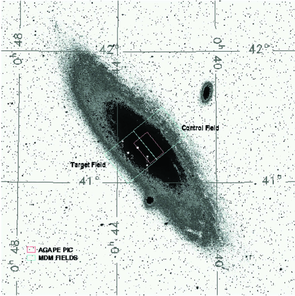
Figure 1: M31 with MDM and Agape observation fields (courtesy of A. Crotts). White stars and dots give, respectively, the position of the five microlensing candidate events (labelled as in Table 2 and where candidates 1 and 2 appear to be superimposed) and of the nova.

Pixel lensing is an efficient tool for searching microlensing events when the sources can not be resolved. In this case, the light collected by each pixel is emitted by a huge number of stars. Although, in principle, all stars in the pixel field are possible sources, one can only detect lensing events due either to bright enough stars or to high amplification events. Typical sources are red giant stars with $M_{I}\in[-3.5,0]$. We estimate that there are about $100$ sources per square arc second that fit these requirements. The main drawback of the method is that usually we have no direct knowledge of the flux of the unamplified source.

For images obtained by the observation of dense stellar fields, the flux collected by a pixel is the sum of the fluxes emitted by single stars, which all contribute to the background. If one of these stars is lensed, its flux varies accordingly. Whenever this variation is large enough, it will be distinguishable from the background produced by the other stars. Denoting by $\phi$ the amplified flux detected by the pixel and by $\phi_{bkg}$ the background flux, the flux variation is given by

$$\phi-\phi_{bkg}=\phi^{*}\left[A(t)-1\right]\,,$$ (2.1)

where $A(t)$ represents the amplification as a function of time,

$$\phi_{bkg}=\phi^{*}+\phi_{res}\,,$$ (2.2)

$\phi^{*}$ is the flux of the star before lensing, and $\phi_{res}$ is that given by the other stars. In the point-like and uniform–motion approximations, $A$ is related to the lensing parameters by:

$$A=\frac{u^{2}+2}{u\sqrt{u^{2}+4}}\,,$$ (2.3)

$$u^{2}=\frac{(t-t_{0})^{2}}{t_{\textrm{E}}^{2}}+u^{2}_{0}\,,$$ (2.4)

where $t_{{\textrm{E}}}$ is the Einstein time, $u_{0}$ the impact parameter in units of the Einstein radius $R_{{\textrm{E}}}$, and $t_{0}$ the time of the maximum amplification. The Einstein radius is

$$R_{{\textrm{E}}}=\sqrt{\frac{4GM}{c^{2}}\frac{D_{ol}D_{ls}}{D_{os}}}\,,$$ (2.5)

where $M$ is the mass of the lens, $D_{ol}$, $D_{os}$ and $D_{ls}$ are the observer-lens, observer-source, and lens-source distances, respectively.

Two characteristic features of a microlensing event are achromaticity and the uniqueness of its luminosity bump, although differential amplification of extended sources can give rise to a chromatic, but still symmetric, lensing light curve (Han et al. 2000).

3 Observations and experimental setup

The data analysed in this paper have been collected on the 1.3 meter McGraw-Hill Telescope, at the MDM observatory, Kitt Peak (USA). Two fields have been observed, which lay on the two sides of the galactic bulge (see Fig. 1) and have been chosen in order to be able to study the expected gradient in the optical depth. The two fields are almost parallel to the major axis of M31; their centers are located at $\alpha=$ 00h43m24s, $\delta=41^{\!\circ}\,12^{\prime}\,10^{\prime\prime}$ (J2000) (named “Target”), and $\alpha=$ 00h42m14s, $\delta=41^{\!\circ}\,24^{\prime}\,20^{\prime\prime}$ (J2000) (named “Control”). The data acquired in the Target field are analysed here.

Fig. 1 shows the location of the fields and for comparison also the smaller AGAPE field. The observations were taken with a CCD camera of $2048\times 2048$ pixels with $0.\hskip-2.0pt^{\prime\prime}5$ and therefore a total field size of $17^{\prime}\times 17^{\prime}$.

In order to test for achromaticity, images have been taken in two bands, a wide $R$ and a near–standard $I$. The exposure time is 6 minutes for $R$, 5 minutes for $I$. The observations started in the fall of 1998 and are still underway.

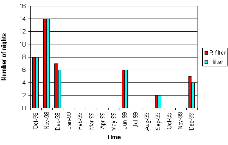
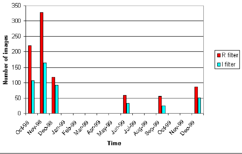
Figure 2: Time sampling for the observations in the “Target” field.

Here we analyse the data taken in the period from the beginning of October 1998 to the end of December 1999. In Fig. 2 we give the time sampling of the measurements (number of nights and images). For each night we have measurements in both $R$ and $I$. On average, there are twice as many $R$ images as $I$ images. In $R$ band we have $\sim 800$ images distributed along 42 nights of observation.

Most of the observations (about $80\%$) are concentrated in the first three months, so that, unfortunately, the time distribution of the data is not optimized for the study of microlensing effects. Thus, the given time distribution allows us to select events that take place almost exclusively during the first three months of observation. Furthermore, the time coverage of about 14 months is still not long enough to test conclusively the bump uniqueness requirement for a microlensing event. Mainly for this reason, we will speak in this paper only of candidate microlensing events.

Taking into account the transmission efficiency of the filters and the catalogued magnitudes $R_{c}$ and $I_{c}$ (Cousins colour system), for a sample of $23$ reference secondaries identified in the Target field (Magnier et al. 1993), we derive the following photometric calibrations

$$R_{c}=m_{R}-0.13\cdot\left(m_{R}-m_{I}\right)+22.54\,,$$ (3.6)

$$I_{c}=m_{I}-0.02\cdot\left(m_{R}-m_{I}\right)+22.21\,,$$ (3.7)

where $m_{R(I)}=-2.5\cdot\log(\phi^{*}_{R(I)})$ and $\phi^{*}_{R(I)}$ is the flux of the source in $ADU/s$ measured in the $R$ and $I$ filters respectively. The estimated error is $\simeq 0.1$ mag, both for $R$ and $I$.

4 Data reduction

During each night of observation about 20 images are taken in $R$ and 12 in $I$. In principle, this allows two possible strategies for the analysis. We can study flux variations on light curves built either by a point obtained from each image, or by a point obtained by averaging over many images. In the first case, we are potentially sensitive to very short time variations. However, this sensitivity is undermined by the low signal-to-noise ratio (S/N). In the second case, the S/N is increased by the square root of the number of images we combine.

Results of the analysis of light curves built with one point per image will be discussed in a future paper. Here we concentrate on the analysis of light curves obtained after combining all the images taken in the same night, using a simple averaging procedure performed on geometrically aligned images (see below).

Data reduction is carried out as follows. After the usual corrections for instrumental effects, debiasing and flatfielding, we normalize all the images to a common reference to cope with variations induced by the observational conditions which are different from image to image (so that we get global stability conditions on each image with respect to a given one). We can distinguish three separate effects: the geometric offset of each image with respect to the others, the difference in photometric conditions of the sky and seeing effects.

By means of geometrical alignment we obtain that each pixel, on all the images, is directed towards the same portion of M31. We take advantage of the fact that the mean seeing disk is much larger than the pixel size. We follow Ansari et al. (1997), and get a precision better than $0.\hskip-2.0pt^{\prime\prime}1$.

Following the methods developed by the AGAPE collaboration (Ansari et al. 1997), we then bring all the images to the same photometric conditions in such a way that the images are globally normalized to a common reference. The procedure is based on the hypothesis that a linear relation exists between “true” and measured flux. It then follows that

$$\phi^{pixel}_{ref}(i,j)=a_{curr}\,\cdot\phi^{pixel}_{curr}(i,j)+b_{curr}\,,$$ (4.8)

where $\phi^{pixel}_{ref}(i,j)$ and $\phi^{pixel}_{curr}(i,j)$ are the fluxes in pixel $(i,j)$ for the reference and the current image, and $a_{curr}$ and $b_{curr}$ are two correction coefficients, which are the same for all the pixels of the image, that take into account the effects of variable atmospheric absorption and variable sky respectively.

The seeing effect gives rise to a spread of the received signal. In our data the seeing varies from $\sim 1.\hskip-2.0pt^{\prime\prime}3$ up to $\sim 2.\hskip-2.0pt^{\prime\prime}2$. Consequently we observe fake fluctuations on light curves obtained after photometrical alignment. In order to cope with this effect, and thus to get reasonably stable light curves, we follow a two steps procedure (for further details see Ansari et al. (1997) and Le Du (2000)). We begin by substituting the flux of each pixel with the flux of the corresponding superpixel, defined as the flux received on a square of $m\times m$ pixels around the central one. The value $m$ should be large enough to cover the typical seeing disk, but not too large to avoid an excessive dilution of the signal. Given the mean seeing value and the angular size of the pixel, we choose $m=5$. This corresponds to $2.\hskip-2.0pt^{\prime\prime}5$, compared to the average value for the seeing of $\sim 1.\hskip-2.0pt^{\prime\prime}7$ for both $R$ and $I$ images. In this way we get a substantial gain in stability since elementary pixels are strongly affected by seeing fluctuations.

Denoting by $\Phi(i,j)$ the flux in a superpixel, we have

$$\Phi(i,j)=\sum_{k=i-n}^{i+n}\sum_{l=j-n}^{j+n}\phi^{pixel}(k,l),$$ (4.9)

where $n=(m-1)/2$ and $m$ is the superpixel size.

Instead of trying to evaluate the point spread function of the image, as a second step we apply an empirical stabilization of the difference between the flux measured on the image and that of the median image, obtained by removing small scale variations with a median filter on a very large window of $31\times 31$ pixels (in this way we get an image whose signal is independent from the seeing value). The stabilization is then based on the observed linear correlation, for each superpixel, between these differences measured on the current image (after photometrical alignment) and the reference image. Denoting with $\Phi_{ref}(i,j),\,\Phi_{curr,a}(i,j)$ and $\Phi^{med}(i,j)$ the value of the flux in a superpixel $(i,j)$ for the reference, the current (photometrically aligned) and the median images respectively, we have the empirical relation

$${\Phi}_{curr,a}(i,j)-{\Phi}^{med}_{curr,a}(i,j)=$$

$$\alpha_{curr}\,\cdot\left[\Phi_{ref}(i,j)-\Phi^{med}_{ref}(i,j)\right]\,.$$ (4.10)

The slope $\alpha_{curr}$, calculated with a minimization procedure, shows a clear correlation with the seeing (Fig. 3). This variation is expected because the flux of a star that enters a superpixel changes with the seeing.

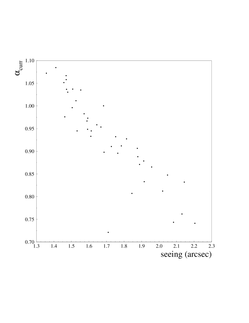
Figure 3: The value of the correction factor $\alpha_{curr}$ in the relation (4) for each composed image as a function of the seeing.

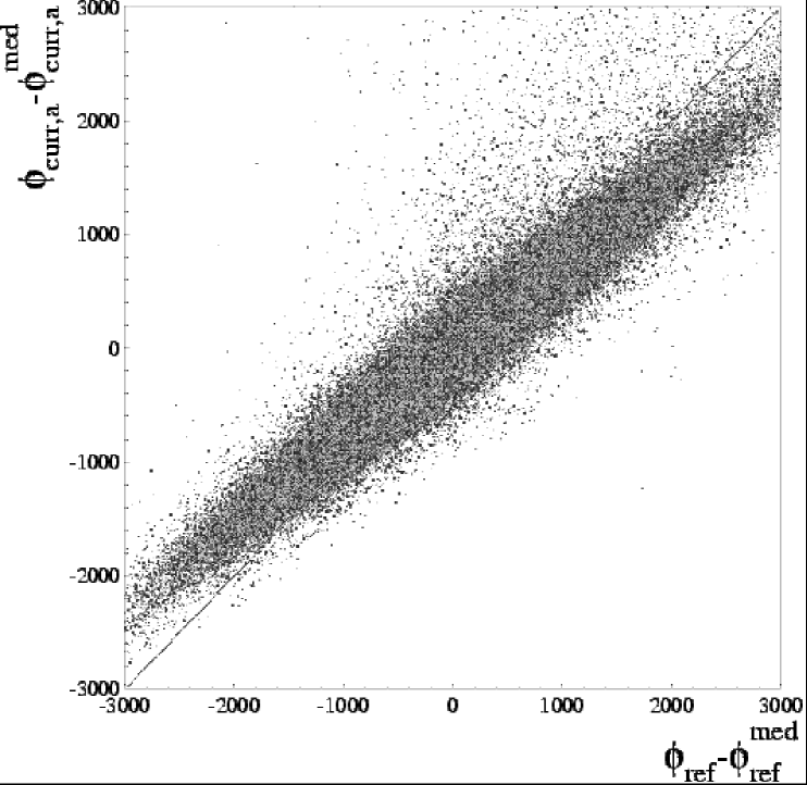
Figure 4: Plot showing the linear correlation between the quantities $\left[\Phi_{curr,a}(i,j)-\Phi_{curr,a}^{med}(i,j)\right]$ and $\left[\Phi_{ref}(i,j)-\Phi_{ref}^{med}(i,j)\right]$. The dashed line is the $y=x$ line.

In the example shown in Fig. 4 the seeing of the current image is greater than that of the reference image, and we find $\alpha_{curr}<1$. We note that in this case, the flux of superpixels for which $\Phi_{curr,a}<\Phi_{curr,a}^{med}$ are corrected to a lower value (points in the bottom left corner), while, if $\Phi_{curr,a}>\Phi_{curr,a}^{med}$, they are corrected up (points in the up right corner). If the seeing of the current image is smaller than that of the reference image ($\alpha_{curr}>1$) the situation is reversed.

While stressing its empirical character, we note that this approach is rapid and efficient. In Fig. 5 we show the effect of the correction on a given light curve.

Figure 5: The same light curve before (top) and after seeing correction. In both cases the error bar shows just the photon noise.

To construct a corrected current pixel flux as close as possible to the reference flux, $\Phi_{ref}$, we replace $\Phi_{ref}$ in (4) by the corrected current flux $\hat{\Phi}_{curr}$ and solve for the latter:

$$\hat{\Phi}_{curr}(i,j)-\Phi^{med}_{ref}(i,j)=$$

$$\frac{1}{\alpha_{curr}}\,\cdot\left[\Phi_{curr,a}(i,j)-\Phi^{med}_{curr,a}(i,j)\right]\,.$$ (4.11)

That is, the corrected flux for the current image is given by the sum of the median of the reference image, and of the weighted deviation from its median, i. e. by its characteristic small spatial scale variations, depending on the relative absorption and on the seeing conditions.

Figure 6: The dispersion for the distribution (4.12) calculated for each composed image as a function of the seeing before ($\sigma_{curr,before}$) and after ($\sigma_{curr,after}$) seeing correction (taking all the points of the image) and for the sample of points selected according to the condition (4.15).

In order to minimize the deviations from the median, we choose as a reference image (one for each filter), an image characterized by a seeing value equal to the average value over the period of observations. The seeing fraction of a source in a superpixel is then $\simeq 0.87$.

Another crucial point is the evaluation of the error to be associated with the received flux. In order to give a more appropriate, though empirical, error estimate, we renormalize the photon noise $\sigma_{stat}$ by introducing a correction factor $\eta_{curr}$, that depends on the image, to include all the systematic effects over which we have less control. For a discussion on the relation between the photon noise and others different systematic effects such as surface brightness fluctuations see Gould (1996).

The evaluation of $\eta_{curr}$ is based on the study of the dispersion of the distribution of the normalized difference, superpixel by superpixel, between the current and the reference image

$$\frac{\hat{\Phi}_{curr}(i,j)-\Phi_{ref}(i,j)}{\sigma_{stat}[\hat{\Phi}_{curr}(i,j)-\Phi_{ref}(i,j)]}\,,$$ (4.12)

where the denominator is the statistical error on the difference.

This distribution is expected to have zero mean (which follows from the geometrical and photometrical alignment) and dispersion one (which would indicate that the photon noise alone gives the right evaluation of the error). We do find a null mean but the dispersion is greater than one and depends on the seeing value. We note, however, that this effect is greatly reduced by the seeing correction (see Fig. 6). For the reference image we assume that the estimated error $\sigma_{est}[\Phi_{ref}]$ coincides with the statistical error given by the photon noise,

$$\sigma^{2}_{est}\left[\Phi_{ref}(i,j)\right]=\sigma^{2}_{stat}\left[\Phi_{ref}(i,j)\right]\,,$$ (4.13)

because it does not suffer from additional noise due to geometric, photometric and seeing transformations, as do the other images. On the other hand, this means that we evaluate the estimated error with respect to that of the reference image.

The correction factor $\eta_{curr}$ is then equal to the dispersion of the distribution (4.12) calculated for a sample of points, properly selected according to the criterion that they belong to “stable” light curves, in order to exclude light curves which show real stellar flux variations. If the subset is small enough and homogeneous, the correction factor appears to be, as expected, almost independent of the seeing value, and has an average value $\eta_{curr}\sim 1.4$ (Fig. 6, bottom). The estimated error of the $(i,j)$ superpixel is obtained from the relation

$$\sigma^{2}_{est}\left[\hat{\Phi}_{curr}(i,j)-\Phi_{ref}(i,j)\right]=$$

$$\eta^{2}_{curr}\,\cdot\sigma^{2}_{stat}\left[\hat{\Phi}_{curr}(i,j)-\Phi_{ref}(i,j)\right]\,.$$ (4.14)

The “stable” pixels are selected by imposing the condition

$$\frac{\bar{\Phi}(i,j)-\bar{\Phi}_{bkg}(i,j)}{\sigma_{stat}[\bar{\Phi}(i,j)-\bar{\Phi}_{bkg}(i,j)]}\leq\epsilon\,,$$ (4.15)

where $\bar{\Phi}(i,j)$ is the average flux along the light curve, $\bar{\Phi}_{bkg}(i,j)$ is the baseline level and $\sigma_{stat}[\bar{\Phi}(i,j)-\bar{\Phi}_{bkg}(i,j)]$ is the error associated with the evaluation of the averages. The baseline is defined as the minimum value taken by the average flux calculated along $q$ consecutive points on the light curve. We take $q=6$, in order to avoid underestimation of the baseline due to fluctuations. Choosing $\epsilon\sim 1.5$, the selected points are $\sim 3\%$ of the total.

5 Candidates selection

A microlensing event is characterized by specific features that distinguish it from other, much more common, types of luminosity variability, the main background to our search. In particular for a microlensing event the bump

• does not repeat;

• follows the (symmetric) Paczyński shape;

• is achromatic.

Variable stars usually show multiple flux variations and have an asymmetric chromatic shape. Moreover, different classes of variable stars are characterized by specific features, such as timescale variation and color, that can be used to distinguish them from real microlensing events.

In the following we devise selection techniques that make use of these characteristics while taking account of the specific features of our data set.

5.1 Bump detection

As a first step we select light curves showing a single flux variation. We begin by evaluating a baseline, i.e. the background flux ($\bar{\Phi}_{bkg}$) along each light curve, as defined in $\S$ 4.

Once the baseline level has been fixed, we look for a significant bump on the light curve. This is identified whenever at least 3 consecutive points exceed the baseline by $3\,\sigma$. The variation is considered to be over when 2 consecutive points fall below the $3\,\sigma$ level. Under the hypothesis that the points follow a gaussian distribution around the baseline, we use the estimator $L$, the likelihood function, to measure the statistical significance of a bump. We want to give more weight to points that are unlikely to be found, so that we define $L$ as

$$L=-\ln\left(\Pi_{j\in bump}P(\Phi|\Phi>\Phi_{j})\right)\;\;\mbox{given}\;\;\bar{\Phi}_{bkg},\,\sigma_{j}\,,$$ (5.16)

where

$$P(\Phi|\Phi>\Phi_{j})=\int_{\Phi_{j}}^{\infty}d\Phi{\frac{1}{\sigma_{j}\sqrt{2\pi}}}\exp\left[{-\frac{(\Phi-\bar{\Phi}_{bkg})^{2}}{2\sigma_{j}^{2}}}\right].$$ (5.17)

$L$ is then a growing function of the unlikelihood that a given variation is the product of random noise. This estimator is different from the usual definition leading to a $\chi^{2}$ with $n$ points, and has the advantage to give weight only to the positive deviations above threshold, which are the ones of interest.

For each light curve we denote by $L_{1}$ and $L_{2}$ the two largest deviations, respectively. We fix a threshold $L_{tresh}$, and we require $L_{1}>L_{tresh}$ to distinguish real variations from noise. Moreover, we fix an upper limit to the ratio $L_{2}/L_{1}$ to exclude light curves with more than one significant variation. The shape analysis is then carried out on the superpixels that have the highest values of $L$ in their immediate neighborhood since we find a cluster of pixels associated with each physical variation. This method suffers from a possible bias introduced by an underestimation of the baseline level (which we further analyse in the next section).

We have carried out a complete analysis selecting the pixels with the following criteria:

• exclusion of resolved stars;

• $L_{tresh}=100$;

• $L_{2}/L_{1}<0.1$.

This selection is made only on $R$ images in order to reduce contamination by variable sources. In this way we take advantage of the fact that most luminous variables (to which we are anyway sensitive) show stronger variations in the $I$ than $R$ band.

By using these peak detection criteria, the number of superpixels is reduced from $\sim 4\cdot 10^{6}$ to $\sim 5\cdot 10^{3}$.

5.2 (Achromatic) shape analysis

As a second step we determine whether the selected flux variation is compatible with a microlensing event.

The light curve of a microlensing event with amplification $A(t)$ due to a source star with unlensed flux $\phi^{*}$ (now to be evaluated in a superpixel) is

$$\Phi(t)=\Phi_{bkg}+\left(A(t)-1\right)\,\phi^{*}\,,$$ (5.18)

where $\Phi(t)$ represents the flux collected in the superpixel associated with a single pixel, as defined before, and $A(t)$ is given by (2.3).

Actually, one can not directly and easily measure $\phi^{*}$, the unamplified flux of the unresolved source star. Only a combination of the 5 parameters that characterize the light curve can be measured in a straightforward manner:

• $\Phi_{bkg}$, the background level (which include the flux of the unamplified source);

• $t_{0}$, the time of maximum amplification;

• $t_{1/2}=t_{1/2}\left(t_{\textrm{E}},\,u_{min}\right)$, the time width of the bump at half–maximum;

• $\Delta\Phi_{max}=\Delta\Phi_{max}\left(\phi^{*},\,u_{min}\right)=\phi^{*}\,(A_{max}-1)$, the excess of the flux with respect to the background at maximum.

Whenever the amplification is high enough, one can approximate $A\left(t\right)\simeq 1/u\left(t\right)$ and $t_{1/2}\simeq 2\sqrt{3}\,t_{\textrm{E}}\,u_{min}$. It is then possible to rewrite the expression (5.18) in terms of these 4 parameters, and a degeneracy arises among the parameters of the amplification $u_{0}$ and $t_{\textrm{E}}$, and the unknown flux of the unamplified source, $\phi^{*}$ (“degenerate” Paczyński curve Gould (1996)). Because of this degeneracy it is in general difficult to get, without extra-information, a reliable insight into all the parameters that characterize the light curve, the Einstein time in particular. For this reason we can extract only the 4 aforementioned parameters even though we carry out a non linear fit with the complete 5 parameters (“non-degenerate”) Paczyński curve.

We now refine the selection based on the likelihood estimator in order to remove unwanted light curves with low S/N and for which the available data do not allow us to well characterize the bump. To this end we perform a Paczyński 5–parameters fit and we study

• the signal to noise ratio for the $R$ flux variation;

• the sampling of the data on the bump.

We define the S/N estimator as

$$Q\equiv\frac{\chi^{2}_{const}-\chi^{2}_{ml}}{\chi^{2}_{ml}/n.d.f}\,,$$ (5.19)

where $\chi^{2}_{const}$ is the $\chi^{2}$ with respect to a constant flux and $\chi^{2}_{ml}$ is the $\chi^{2}$ with respect to the Paczyński fit.

The ratio $Q$ is actually correlated with the likelihood estimator $L$ we used in the previous step. In parallel with the cut $L_{1}>100$ we then keep only light curves with $Q>100$.

We do not ask for the $I$ bump to be significant.

The second point concerns the necessity to well characterize the bump shape in order to recognize it as a microlensing event in the presence of highly irregular time sampling of data (see Fig. 2). For this purpose we require at least 4 points on both sides of the maximum, and at least 2 points inside the interval $t_{0}\pm t_{1/2}/2$.

After this selection we are left with 1356 flux variations.

From now on we work with the data in both colors ($R$ and $I$) and we carry out a shape analysis of the light curve based on a two steps procedure as follows:

• $\chi^{2}$ selection criterion;

• Durbin-Watson test on residuals;

which we now discuss in some detail.

The first point is taken into account by performing the non-degenerate Paczyński fit in both colors simultaneously, so that we check also for achromaticity of the selected luminosity variations. In particular, we require that the three geometrical parameters that characterize the amplification ($t_{\textrm{E}},\,u_{0}$ and $t_{0}$) be the same in both colors. We get, therefore, a 7 parameters least $\chi^{2}$ non linear fit:

$$\chi^{2}=\sum_{j=1}^{2}\sum_{i=1}^{N_{j}}\frac{\left[\Phi_{j}(t_{i})-\Phi_{model}(t_{i}|\Phi^{j}_{bkg},\phi^{*,j},t_{0},t_{\textrm{E}},u_{0})\right]^{2}}{\sigma_{i,j}^{2}}\,.$$ (5.20)

To retain a light curve as a candidate microlensing event, we require that the reduced $\chi^{2}$

$$\frac{\chi^{2}}{N-7}\equiv\tilde{\chi}^{2}<1.5$$ (5.21)

where $N=N_{R}+N_{I}$ is the total number of points in $I$ and $R$.

The application of the $\chi^{2}$ criterion test reduces the sample of light curves from 1356 to 27.

As a further step we apply the Durbin–Watson (Durbin & Watson 1951) test to the residuals with respect to the 7-parameters non-degenerate Paczyński fit. With the DW test we check the null hypothesis that the residuals are not timely–correlated by studying possible correlation effects between each residual and the next one against type I error (i.e. against the error to reject the null hypothesis although it is correct, e.g. Babu & Feigelson (1996)). We require a significance level of 10%. As time plays a fundamental role in the DW test, we perform this test on each color separately.

We call $dw_{R}$ and $dw_{I}$ the coefficients for the Durbin–Watson test on the full data set. In order to retain a light curve we require $1.54<dw_{R(I)}<2.46$, appropriate for 40–42 points along the light curve.

This statistical analysis reduces our sample of light curves from 27 to 11.

It is worthwhile to note that some light curves, showing a real microlensing event superimposed on a signal due to some nearby variable source, and passing the previous selection criteria, could be excluded by the DW test, sensitive to timely correlated residuals.

In order to test our efficiency with respect to the introduction of the DW test we have done a study on “flat” light curves performing a “constant flux” fit, and selecting light curves requiring a reduced $\tilde{\chi}^{2}<1.5$. By applying the DW test we then reject about 50% of these light curves, i.e., more than the 10% we could expect if we had just random fluctuations. In the discussion of the Monte Carlo simulation we duly take into account this effect.

5.3 Color and timescale selection

criterion	$\%$ pixel excluded	pixel left
exclusion of resolved stars	$\sim 10\%$	$\sim 3.6\cdot 10^{6}$
mono bump likelihood analysis	$\sim 99.8\%$	5269
signal to noise ratio ($Q>100$)	$\sim 69\%$	1650
sampling of the data on the bump	$\sim 18\%$	1356
$\chi^{2}<1.5$	$\sim 98\%$	27
$1.54<dw_{R(I)}<2.46$	$\sim 59\%$	11
$t_{1/2}<40$ d or $R-I<1.0$	$\sim 55\%$	5

Table 1: Summary of selection criteria.

id	$\alpha$(J2000)	$\delta$(J2000)	$t_{1/2}$ (d)	$t_{0}$ (J-2449624.5)	$R_{max}$	$R-I$	$\tilde{\chi}^{2}$	$dw_{R}$	$dw_{I}$
1	00h43m27.4s	$41^{\circ}\,13^{\prime}\,11^{\prime\prime}$	$32\pm 6$	$1506\pm 1$	$22.6\pm 0.1$	$0.3\pm 0.2$	1.25	1.78	1.65
2	00h43m26.5s	$41^{\circ}\,13^{\prime}\,16^{\prime\prime}$	$22\pm 7$	$1508\pm 1$	$22.7\pm 0.1$	$0.2\pm 0.2$	1.37	1.57	1.65
3	00h43m39.9s	$41^{\circ}\,18^{\prime}\,41^{\prime\prime}$	$39\pm 9$	$1505\pm 1$	$22.2\pm 0.1$	$0.8\pm 0.2$	1.48	1.97	1.67
4	00h42m39.3s	$41^{\circ}\,6^{\prime}\,53^{\prime\prime}$	$15\pm 1$	$1470\pm 1$	$22.3\pm 0.1$	$0.5\pm 0.2$	1.42	1.68	1.95
5	00h42m39.1s	$41^{\circ}\,11^{\prime}\,26^{\prime\prime}$	$25\pm 3$	$1501\pm 1$	$21.7\pm 0.1$	$0.5\pm 0.2$	1.16	1.82	1.99

Table 2: Characteristics of microlensing candidates.

By far, the most efficient way to get rid of multiple flux variations due to variable stars is to acquire data that are distributed regularly for a sufficiently long period of time. Unfortunately, at present, the data cover with regularity only the first three months of observation, and the total baseline is less than 2 years long.

For this reason, in addition to the analytical treatment that looks for the compatibility with an achromatic Paczyński light curve (efficient, for instance, to reject nova-like events), we introduce another criterion based on the study of some physical characteristics of the selected flux variations.

In particular we note that long period red variable stars (such as Miras) could not be completely excluded by the selection procedure applied so far. By contrast, short period variable stars are eliminated thanks to the cut on the second bump of the likelihood function. A preliminary analysis of the period, the color and the light curves of long period red variable stars, taken from de Laverny et al. (1997), lead us, with a rather conservative approach, to exclude those light curves that present at the same time a duration $t_{1/2}>40$ days and a color $(R-I)_{C}>1.0$. A more detailed analysis aimed at a better estimation of that background noise is currently underway.

We are aware that this last selection criterion could eliminate some real microlensing events. The probability that this might happen is however low because the microlensing timescales are expected to be uncorrelated with the source color. In fact, a combination of a large $t_{1/2}$ and color $(R-I)_{C}>1.0$ is extremely unlikely for microlensing events, but quite common for red variables.

This last criterion further reduces the number of candidates from 11 down to 5.

5.4 Results of microlensing search

We now summarize (Table 1) the different steps in the selection, give the number of surviving pixels after the application of the indicated criteria and the details of our set of microlensing candidate events.

We take these 5 light curves, whose characteristics we are now going to discuss, as our final selection of microlensing candidate events.

In the following table (Table 2) we give their position, the estimated $t_{1/2}$ in days, the time of maximum amplification $t_{0}$ (J-2449624.5), the magnitude at maximum $R_{max}$ and the color $(R-I)_{C}$. We then give the values of the fit: the reduced $\tilde{\chi}^{2}$ and the values of the Durbin–Watson $dw_{R(I)}$ coefficients.

Figure 7: Light curves of the 5 candidate microlensing events. On the y axis, $\Delta\Phi\equiv\Phi-\Phi_{bkg}$. On the x axis, the origin of time is in J-2449624.5. The dashed line represent the result of the 7–parameters Paczyński fit.

The corresponding light curves are shown in Fig. 7.

5.5 Variable stars

Figure 8: The $R$ and $I$ light curve of the nova event in $\alpha$=00h43m1.7s, $\delta=41^{\circ}\,15^{\prime}\,37^{\prime\prime}$ (J2000).

Our data contain many more varying light curves that are due not to microlensing events but to other variable sources. The study of these variable stars is an interesting task in itself. Clearly, pixel lensing is well suited for this research. We give here (see Fig. 8) only the light curve of an event characterized by a very strong and chromatic flux variation, that has already been considered as due to a nova (Modjaz & Li 1999) and whose light curve is also shown in Riffeser et al. (2001). We note that our points, even if with a poorer sampling in the descent, are in good agreement with those of this collaboration. This nova is found in the region of the bulge of M31 and we localize it in $\alpha$=00h43m1.7s, $\delta=41^{\circ}\,15^{\prime}\,37^{\prime\prime}$ (J2000). We evaluate the magnitude at maximum amplification as $R_{c}=17.0$ and $I_{c}=16.8$.

6 Discussion of microlensing search

In order to gain an insight into the results obtained, we compare our 5 candidate microlensing events with the prediction of a Monte Carlo simulation which takes into account the experimental set up and the time sampling of the observations. We assume a standard model (isothermal sphere with a core radius of 5 kpc) for the haloes of both M31 and the Milky Way. The total mass of M31 is assumed to be twice that of our Galaxy. MACHOs can be located in either haloes. Moreover, we consider also self–lensing due to stars in the M31 bulge or disk. We fix the lens masses at different values for MACHOs in the halo and stars in the bulge or disk. The model of the bulge is taken in Kent (1989), the luminosity function in Han et al. (1998). The luminosity function of the disk is determined considering two models: the one developed in Devriendt et al. (1999) and the model obtained considering the data of the solar neighborhood taken in Allen (1973) corrected for high luminosities (Hodge et al 1988). The results we obtain are almost insensitive to the particular choice between these two models.

We choose the mass of the lenses in the bulge to be $m_{MACHO}^{bulge}=0.4\,M_{\odot}$, and the mass for MACHOs in the haloes equal either to $m_{MACHO}^{halo}=0.5\,M_{\odot}$ or to $m_{MACHO}^{halo}=0.01\,M_{\odot}$. In both cases about $90\%$ of the expected events are due to lenses located in M31. Taking into account our selection criteria, the results for the expected number of events for a halo fully composed of MACHOs, including a contribution due to lensing by stars of the bulge and disk of M31 of $\sim 1$ event independent of halo parameters, is $\sim 4$ and $\sim 9$, respectively. The Monte Carlo simulation does not yet include the effect of secondary bumps due to artifacts of the image processing (alignment, seeing stabilization) and to underlying variable objects. From the data, we estimate that these effects reduce the number of observed events by at most 30%, and this for the shortest events.

We expect, and this is confirmed by simulations, that the sources of most detectable events are red giants and have very large radii. Therefore, finite size and limb darkening effects are important, in particular for low mass lenses. These effects are included in the simulations. However, in both the real and simulated analysis, we do not include finite size and limb darkening effects in the amplification light curve fitted to the events. This results in a loss of detection efficiency smaller than 5%, which is taken into account in the simulations.

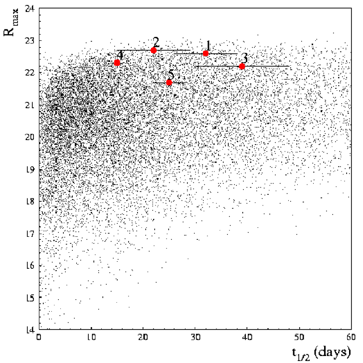
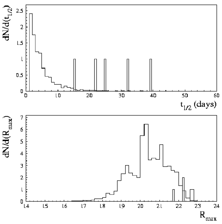
Figure 9: Results of Monte Carlo simulations, $m_{MACHO}^{halo}=10^{-2}\,M_{\odot}$ case. The scale on the y coordinate of the two distributions on the right are in arbitrary units. The dots (left) give the position of the candidates as labelled in Table 2.

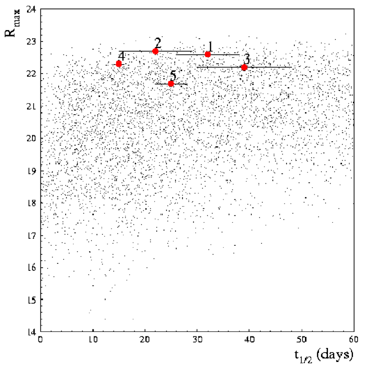
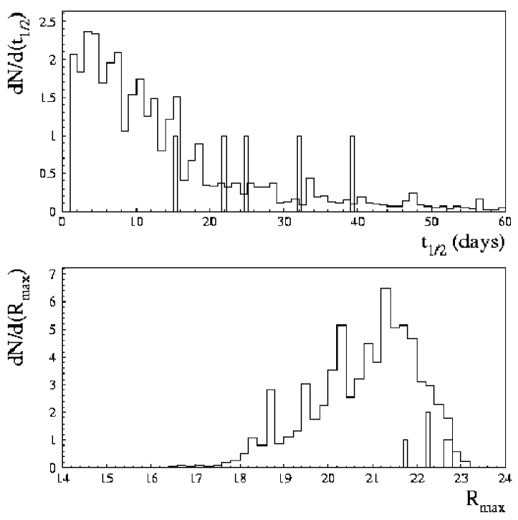
Figure 10: Results of Monte Carlo simulations, $m_{MACHO}^{halo}=0.5\,M_{\odot}$ case. The scale on the y coordinate of the two distributions on the right are in arbitrary units. The dots (left) give the position of the candidates as labelled in Table 2.

Locating our candidates in the parameter space predicted by the simulation is more meaningful. We report the expected values of $t_{1/2}$ and on the $R$ magnitude at maximum. In Figs. 9 and 10 we give plots of their functional relation and of their projected distributions. On these same plots we give the position of our selected light curves in this parameter space.

Looking at the distributions we notice that for the $m_{MACHO}^{halo}=0.5\,M_{\odot}$ and $m_{MACHO}^{halo}=0.01\,M_{\odot}$ cases, $80\%$ of the light curves are expected to have a time width at half maximum $t_{1/2}<24$ and $t_{1/2}<10$ days, respectively (of course, shorter events are expected when the MACHO mass is smaller). In both cases, $\sim 80\%$ of the events are predicted with a magnitude at maximum $R_{max}<21.7$. Our candidates have $t_{1/2}\geq 15$ days and $R_{max}\geq 21.7$ (somewhat at the limit of the expected distributions) and therefore most of them are probably not microlensing events. Still, we expect $\sim 1$ self–lensing event and it is possible that one or two of them are true microlensing events. In any case, from the $t_{1/2}$ distribution, we are led to exclude that the microlensing candidate events are due to MACHOs of very small mass (only $\sim 10\%$ of events with $m_{MACHO}^{halo}=0.01\,M_{\odot}$ are expected to have $t_{1/2}>15$ days). This is indeed in agreement with the results found by the MACHO and EROS collaborations: they find lens masses in the halo within the range 0.2–0.6 $M_{\odot}$ (Alcock et al. 2000; Lasserre et al. 2000).

We are not yet in a position to tell what kind of varying objects generate our events if they are not due to microlensing. They may be irregular or long period variable giants, but only a longer time baseline, and/or observations of the object at minimum light, will allow us to conclude.

The MDM analysis is not yet complete. The results from the analysis of data acquired in the other field (located on the opposite side with respect to the major axis of M31 of the Target field analysed here) and results from new observations scheduled for the fall 2001 will give us the opportunity to gain further insight into the still open question of the composition of dark haloes. At the present time, with the caution suggested by the just mentioned problems, the analysis discussed in this paper tends to confirm that only a minor fraction of dark matter in the galactic haloes is in form of MACHOs within the mass range 0.01–0.5 $M_{\odot}$ under the assumption of a standard model of the halo and given source luminosity functions.

- (1) Alcock, C., et al. 1993, Nature, 365, 621
- (2) Alcock, C., et al. 2000, ApJ, 542, 281
- (3) Allen, C. W., ed. 1973, Astophysical Quantities (London, Athlone Press)
- (4) Alonso, A., et al. 1999, A&AS, 140, 261
- (5) Ansari, R., et al. 1997, A&A, 324, 843
- (6) Ansari, R., et al. 1999, A&A, 344, L49.
- (7) Aubourg, E., et al. 1993, Nature, 365, 623
- (8) Aurière, M., et al. 2001, ApJ, 553, L137
- (9) Babu, G. J., & Feigelson, E. D. 1996, Astrostatistics (Chapman & Hall, London)
- (10) Baillon, P., et al. 1993, A&A, 277, 1
- (11) Calchi Novati, S. 2000, Microlensing gravitazionale per la rivelazione di MACHOs in direzione della galassia M31: analisi dati con il metodo di AGAPE, PhD thesis, University of Salerno
- (12) Crotts, A. P. 1992, ApJ, 399, L43
- (13) Crotts, A. P., et al. 2000, astro-ph/0006282
- (14) de Laverny, P., et al. 1997, A&AS, 122, 415
- (15) Devriendt, J., Guiderdoni, B., & Sadat, R. 1999, A&A , 350, 381
- (16) Durbin, J., & Watson, G. S. 1951, Biometrika, 38, 159
- (17) Gould, A. 1994, ApJ, 421, L71
- (18) Gould, A. 1996, ApJ, 470, 201
- (19) Han, C., Jeong, Y., & Kim, H. 1998, ApJ, 507, 102
- (20) Han, C., Park, S., & Jeong J. 2000, MNRAS, 320, 41
- (21) Hodge, P., Lee, M. G., & Mateo, M. 1988, ApJ, 324, 172
- (22) Jetzer, Ph. 1994, A&A, 286, 426
- (23) Kent, S. M. 1989, AJ, 97, 1614
- (24) Le Du, Y. 2000, AGAPE: L’effet de microlentille gravitationnelle pour la recherche de matière noire sous forme de MACHOs en direction de la galaxie M31, PhD thesis, Paris
- (25) Magnier, E. A., et al. 1993, A&A, 272, 695
- (26) Lasserre, T., et al. 2000, A&A, 355, L39
- (27) Modjaz, M., & Li, W. D. 1999, IAU Circ., 7218, 2
- (28) Paczyński, B. 1986, ApJ, 304, 1
- (29) Riffeser, A., et al. 2001, astro-ph/0104283
- (30) Udalski, A., et al. 1993, Acta Astronomica, 43, 289
- (31) Tomaney, A., & Crotts, A. P. 1994, BAAS, 185, # 17.01
- (32) Witt, H. J., & Mao, S. 1994, ApJ, 430, 505