Image reduction pipeline for the detection of variable sources in highly crowded fields

We present a reduction pipeline for CCD (charge-coupled device) images which was built to search for variable sources in highly crowded fields like the M 31 bulge and to handle extensive databases due to large time series. We describe all steps of the standard reduction in detail with emphasis on the realisation of per pixel error propagation: Bias correction, treatment of bad pixels, flatfielding, and filtering of cosmic rays. The problems of conservation of PSF (point spread function) and error propagation in our image alignment procedure as well as the detection algorithm for variable sources are discussed: We build difference images via image convolution with a technique called OIS (optimal image subtraction, Alard & Lupton, 1998), proceed with an automatic detection of variable sources in noise dominated images and finally apply a PSF-fitting, relative photometry to the sources found. For the WeCAPP project (Riffeser et al., 2001) we achieve $3\sigma$ detections for variable sources with an apparent brightness of e.g. $m=24.9\;\mathrm{mag}$ at their minimum and a variation of $\Delta m=2.4\;\mathrm{mag}$ (or $m=21.9\;\mathrm{mag}$ brightness minimum and a variation of $\Delta m=0.6\;\mathrm{mag}$) on a background signal of $18.1\;\mathrm{mag}/\mathrm{arcsec}^{2}$ based on a $500\;\mathrm{s}$ exposure with $1.5\;\mathrm{arcsec}$ seeing at a $1.2\;\mathrm{m}$ telescope. The complete per pixel error propagation allows us to give accurate errors for each measurement.

1 Introduction

Astronomical imaging in optical wavebands is performed nearly exclusively with charge-coupled devices today. Despite the numerous advantages of modern CCDs, their images still have to be corrected for a couple of disturbing influences and effects before one can base advance in science on them. Here, we will focus on the problems arising with optical, ground based imaging and time-series observations to find and measure variable sources either hidden in a bright background (e.g. a variable star in its host galaxy) or a crowded field or even in a combination of both.

The search for variable objects with common photometry methods becomes very ineffective in crowded fields because of blending. Phillips & Davis (1995) show algorithms for registering, matching the point spread functions (PSFs), and matching the intensity scales of two or more images in order to detect transient events. Tomaney & Crotts (1996) propose a method called Difference Image Analysis (DIA) where the point spread function (PSF), describing the projection of a point source onto the image plane, is matched by calculating a convolution kernel in Fourier space. The application to real data has been shown for Galactic Microlensing (Alcock et al., 1999) as well as for microlensing in M 31 (Crotts et al., 1999). A new method for Optimal Image Subtraction (OIS) of two images has been designed by Alard & Lupton (1998). They derive an optimal kernel solution from a simple least-squares analysis using all pixels of both images. This method has been used successfully by different projects (Wozniak, 2000, OGLE,; Bond et al., 2001, MOA,; Mochejska et al., 2001, DIRECT,; etc.).

origin	property
Detector:	Photosensitive area and additional “borders” (prescan, postscan, overscan), geometric variation of pixel size and edge pixels, pixel sensitivity variations and pixel defects (cold pixel, hot pixel, trap), sub-pixel quantum efficiency variations, charge transfer efficiency (CTE), linearity range and saturation level.
Electronics:	Bias, gain, ADC width, sampling (of charges), thermal noise.
Instrument:	Dust in optics and optic distortions, optical scale and detector pixel size (and their ratio to the typical seeing – spatial sampling), file format (e.g. FITS ), and information beyond raw image (header keywords).
Environment:	Signals originating from particle events (cosmic rays), varying meteorological observing conditions (seeing), and other atmospheric effects like sky illumination (moon) and extinction.

Table 1: Properties of raw CCD images and their origin.

We have expanded OIS with a standard reduction pipeline, a finding algorithm for variable sources, a PSF-fitting photometry, and per pixel error propagation for all steps of image processing. We are able to give accurate errors for each photometric measurement of a variable source beyond an estimate based on the noise in a single difference image. Our software has been developed to deal with time series obtained with the 0.8 m Wendelstein telescope and the Calar Alto 1.23 m telescope to monitor variable stars and find microlensing events towards the M 31 bulge in the first instance. However, we stress that many of the procedures presented here may also be applied directly to other types of astronomical imaging.

The first part of this paper motivates the effort to implement per pixel error propagation. The second part gives a detailed description of our standard reduction for CCD frames. In the third part we present our image alignment procedure. The fourth part describes the image convolution with OIS, the detection procedure for variable sources and the relative photometry of those sources. In the last section we give the results of performance tests on simulated images.

2 Motivation for per pixel error propagation

2.1 Properties of raw CCD images

We have to consider all properties of raw CCD images (Tab. 1) before we can establish a reliable difference image analysis. When estimating photometric errors all these effects and their errors have to be considered again in addition to the photon noise induced by the objects imaged. To account for those additional photometric errors the error has to be calculated and propagated for each pixel and every data reduction step applied.

2.2 Error propagation – an analytic example

We show that the errors resulting e.g. from flatfield calibration (Sect. 3.7) may be dominant for bright objects or inadequate flatfields which cannot always be avoided. Statistics for this effect on simulated images are shown in Sect. 6.1. (See Tab. 2 for common components of formulae used throughout this article.)

$(x,y)$	=	pixel coordinates,
$I(x,y)$	=	value of pixel $(x,y)$ in image $I$,
$\delta_{I}(x,y)$	=	corresponding absolute error,
$\tilde{I},\;\hat{I},\;\bar{I}$	=	sequence of indicators, that some reduction step
		has been applied to $I$,
$n_{I}$	=	integer number of e.g. images of type $I$,
$\sigma$	=	the root mean square of a sample.

Table 2: Common components for the notation of formulae.

One can estimate this effect assuming $n_{I}$ images, each with $I(x,y)$ detected photons per pixel, and $\delta_{I}(x,y)=\sqrt{I(x,y)}$ error per pixel, so the preliminary error estimate for a per pixel added stack

$$\tilde{I}(x,y)=\sum_{j=1}^{n_{I}}\frac{I_{j}(x,y)}{F(x,y)}\approx n_{I}\;\frac{I(x,y)}{F(x,y)}$$ (1)

(where “$\approx$” is due to the fact that the $I_{j}$ will vary, and $F(x,y)\approx 1$) is

$$\delta_{\tilde{I}}(x,y)\approx\delta_{I}(x,y)\;\sqrt{n_{I}}\;.$$ (2)

Including as further assumptions a flatfield error $\delta_{F}(x,y)$, a ratio of the relative errors between the flatfield and a single image given by

$$\xi(x,y)=\frac{\delta_{I}(x,y)}{I(x,y)}\left/\frac{\delta_{F}(x,y)}{F(x,y)}\right.\;,$$ (3)

and Gaussian error propagation, we can calculate the impact of flatfield calibration on the error $\delta_{\tilde{I}}(x,y)$ of the stack. The propagated per pixel error depends on the individual signal-to-noise ratios of the images and the flatfield, and on dithering. When stacking spatially undithered images, the flatfield error $\delta_{F}(x,y)$ of the same pixel $(x,y)$ adds to each individual image $I(x,y)$, so the flatfield error part of the stack is not an independent error. It is like stacking first and flatfielding subsequently:

$$\delta_{\tilde{I}}(x,y)\approx\delta_{I}(x,y)\;\sqrt{n_{I}\left(1+\frac{n_{I}}{\xi^{2}}\right)}\;.$$ (4)

With spatially dithered (and digitally realigned) images we get (by neglecting the effects of the alignment procedure)

$$\delta_{\tilde{I}}(x,y)\approx\delta_{I}(x,y)\;\sqrt{n_{I}\left(1+\frac{1}{\xi^{2}}\right)}\;,$$ (5)

because different and therefore independent flatfield pixels add to the per pixel error of the stack.

An example: We consider an extended and bright object (e.g. the M 31 bulge), and twilight flatfields. Here we get $1<\xi<3$ because of the difficulties in getting twilight flats discussed in Sect. 3.7. In a dithered, $n_{I}=5$ stack this yields an up to $41\%$ error increment and even a $145\%$ increment in an undithered, $n_{I}=5$ stack, both compared to the simple estimate of Eq. 2, i.e. with respect to the Poissonian noise in the images alone.

Now we treat a complementary case: When imaging faint objects in empty fields, the lack of proper flatfields pushes observers to build flatfields using the skylight in the (dithered) images. With $I(x,y)=\mathrm{object}(x,y)+\mathrm{sky}(x,y)$ and $n_{F}$ of $n_{I}$ images usable for building the flat ($n_{F}<n_{I}$ because of the objects and cosmics in the field) we get

$$\delta_{\tilde{I}}(x,y)\approx\delta_{I}(x,y)\;\sqrt{n_{I}\left[1+\frac{1}{n_{F}}\left(1+\frac{\mathrm{object}(x,y)}{\mathrm{sky}(x,y)}\right)\right]}$$ (6)

for the error in a stack, using

$$\frac{\delta_{F}(x,y)}{F(x,y)}=\frac{1}{\sqrt{n_{F}\mathrm{sky}}}\quad\mbox{in Eq.\leavevmode\nobreak\ \ref{e.flatdithered}.}$$ (7)

For $n_{F}=5$ images, which can be used in every pixel for flatfielding, and with an object which is much fainter than the sky, this yields a $10\%$ error increment (here, and below again, compared to the naive, Poissonian noise estimate of Eq. 2). Assuming an object with flux comparable to the sky, the error increment already exceeds $18\%$.

The per pixel propagation of errors gets even more important when performing multi-pixel approximations, as we do in some parts of our data reduction pipeline for the difference image analysis. When performing e.g. PSF-fitting one can enhance the accuracy by including the appropriate error weights as stated in Sect. 6.6.

3 Standard reduction pipeline for images

We start with the standard reduction for individual object frames. All effects of Sect. 2.1, which can be corrected in single images, will be discussed. We show a way how to compensate for these effects, and, in addition, how these compensations affect the total error budget of each pixel.

3.1 Saturation

Saturated pixels (due to ADC saturation or due to pixel charges at full well capacity) have to be marked as wrong value pixels. With a reasonable bias adjustment no pixel should have a zero value, so we set saturated pixels to zero as a first step. Since one cannot know if a saturated pixel has or has not bloomed, the four directly adjacent neighbouring pixels should also be treated like saturated. Depending on the specific properties of a CCD, the blooming assumption may be restricted to the two pixels in-and-against the row-shift direction. As we perform the bias correction (Sect. 3.2) and the initial calculation of an error frame (Sect. 3.3) in one step, the zero marked pixels will still be recognised after the bias has been subtracted. Pixels with values beyond the linearity range of the CCD have to be corrected, or, if not possible, also have to be treated like saturated pixels. Since we do not have to treat images with values in the non linear regime we will not provide error propagation for this case.

3.2 Bias correction

The bias originates from the offset voltage of the CCD ADC. Depending on its properties we remove it following two subsequent approaches:

• If the patterns in the bias frame are varying on short time scales, or there is no pattern at all (just thermal noise), we subtract only the $\kappa\sigma$-clipped mean of a suitable part of the overscan (i.e. a part of the overscan, which is identical in exposed frames and dark, not exposed frames). Since the bias is an additive constant and mostly a small number the $\kappa\sigma$-clipped mean ($\kappa\approx 6$, to get rid of cosmics) will be more accurate than the median.

• If the bias patterns are reproducible, we subtract in addition a $\kappa\sigma$-median-clipped mean image of overscan corrected bias frames. (We check the reproducibility by looking for patterns in such a mean image; see Sect. 3.7 for details on $\kappa\sigma$-median-clipping.)

Three types of errors have to be considered when correcting for the bias:

• Statistical error: The readout noise consists of the thermal noise of the amplifier, and, if present, of the dark current.

• Systematic error: Unreproducible bias patterns may result from bad CCD electronics or insufficient electronic shielding. (Strong radio immission may even penetrate an excellent shielding.)

• Numerical error: Error resulting from the numerical determination of the bias level.

Additional errors (e.g. count dependent bias) may arise because of a bad CCD or bad electronics, but dealing with those is beyond our scope. Fortunately we also had no significant dark current to deal with on any of the CCDs we have used so far.

3.3 Generation of the error frame

Our error frames are similar to a data-quality mask as used in many pipelines, but differ in that their values are not representative flags but actually numerical errors, with the exception of saturated and bad pixels which are represented by simple flags (-1, 0).

Each pixel $(x,y)$ in an image $I$ has an initial error $\delta_{I}(x,y)$ resulting from the photon noise, the bias noise (i.e. readout noise) plus the error in determination of the bias level:

$$\delta_{I}(x,y)=\sqrt{\frac{\mathrm{counts}_{I}(x,y)-\mathrm{bias}_{I}}{\mathrm{gain}_{I}}+\sigma_{\mathrm{bias}_{I}}^{2}+\frac{\sigma_{\mathrm{bias}_{I}}^{2}}{n_{\mathrm{bias}_{I}}}}\;,$$ (8)

where
$\mathrm{counts}_{I}$ = flux of pixel $(x,y)$ in image $I$ in ADU, $\mathrm{bias}_{I}$ = bias of the image, $\mathrm{gain}_{I}$ = $\frac{\mathrm{photons}_{I}}{\mathrm{ADU}}$ = conversion factor, $\sigma_{\mathrm{bias}_{I}}$ = we use the $\kappa(=6)\sigma$-clipped RMS of a suitable part of the overscan as an estimation for the bias noise (i.e. readout noise), $n_{\mathrm{bias}_{I}}$ = number of pixels actually used for the bias determination.
If using a small clipping factor ($\kappa<3$) for the determination of the bias noise, $\sigma_{\mathrm{bias}_{I}}$ will be underestimated and therefore has to be corrected by a factor $1/C_{C}$ where

$$C_{C}=\mathrm{erf}(\kappa/\sqrt{2})=\frac{1}{\sqrt{2\pi}}\int\limits_{-\kappa}^{\kappa}e^{-\frac{1}{2}\hat{\kappa}^{2}}d\hat{\kappa}\;.$$ (9)

Reproducible bias patterns can be determined with an accuracy only limited by the applied numerical precision, so their error may be neglected.
We mark saturated pixels in the error frame by setting them to minus one, which will be dominant in any error propagation from now on to prevent the use of saturated pixels.

3.4 Defective pixels

We identify defective pixels by checking the specific CCD documentation as well as closely examining flatfields (for cold pixels, traps, and coating defects) and darks (for hot pixels) with a large spread of exposure times and counts if available. All sorts of defective pixels we set to zero and approximate them later (Sect. 3.9); the error is also set to zero.

3.5 Photosensitive region

Since the overscan parts of a frame are not needed any more, the frame is trimmed to its exposed part. We also truncate any bad, first or last rows or columns. On some CCDs the first row is broken and the edges of the photosensitive area behave differently from the rest: The effective size of the edge pixels can be up to $20\%$ larger than the size of an average pixel.

3.6 Low counts pixels

To ensure that only pixel values above an ignorance level will be used, we set low count pixels and their error to zero. This also accounts for the non linear range of a CCD due to a bad charge transfer efficiency (CTE) at low pixel charges. Like the defective pixels (Sect. 3.4) those pixels will be estimated later (Sect. 3.9), where it is possible.

3.7 Flatfield calibration

3.7.1 Flatfielding basics

In order to normalise the apparent photon sensitivity of all pixels in a single CCD frame, a calibration image (flatfield image) has to be built. In an ideal case this would be the image of an extended, homogeneous, flat, and white object at infinity. The apparent photon sensitivity results from geometric size, coating, and electronic properties of each single pixel, and, in addition, from the inherent properties of the optics, and finally dust in the optics. Since there is no feasible way to get near the ideal case with dome flats (any additional optics which would project the nearby dome to infinity would again add features to the calibration image), we decided to stretch our efforts to improve sky flats. The daylight sky is the ideal case for flatfield images, but is much to bright for broadband filter images. Therefore the suitable time for getting sky flats is restricted to dusk and dawn. The superiority of twilight flatfields over dome flatfields is well known and e.g. discussed in Buil (1991), and Mackay (1986). Nevertheless, dome flats and twilight flats can be used effectively in combination as detailed in Sect. 3.7.3.

3.7.2 Observation strategy for flatfields

In order to minimise interfering effects like stars and photon noise, we need at least five flatfield images per filter used, fulfilling these additional constraints:

• The individual flatfield images should have count levels as high or higher than the average of the observed object in a single frame, as their noise adds to the data (see Sect. 2.2 and 6.1). Nevertheless, flatfields with less counts are preferred to having less than five flatfields.

• The exposures have to be long enough to avoid residuals of the shutter (shutter pattern), but still short enough to avoid saturation. If the shutter movements show a predictable time dependency, the flatfields can be deconvolved from the two-dimensional shutter function in a simple way as proposed by Surma (1993). Unfortunately this is not the case with our observations for the WeCAPP project (Riffeser et al., 2001). Since the building of suitable flatfields already is the most (human) time consuming part of the standard reduction phase, we do not go into building shutter patterns for each individual flatfield, but simply exclude underexposed flats and try to manage with the remaining.

• Flatfields should be taken of a blank field to have less stars to be removed.

• The telescope focus should be well adjusted to minimise the number of pixels affected by stars. This is difficult for dusk flatfields, because one cannot make a focus series of a star before starting with the flat series for obvious reasons.

• All flatfields of one series should have some small offsets in orientation, so the $\kappa\sigma$-clipped median of the series will be clean of stars. We found an offset of $30^{\prime\prime}$ to be sufficient.

• Diffuse light contamination (i.e. reflections from inside the dome) has to be avoided. Neglecting this effect results in a mixture of dome and sky flat with improper illumination.

As one can easily estimate, using the Tyson & Gal (1993) twilight formula, it is impossible to get five flatfield images (following above constraints) for more than one filter, if the time needed for CCD wipe and readout exceeds three minutes. For those cases we found the restriction to only take flat series for one filter per twilight, and to alternate the filters for each twilight period, to produce better results than the combination of multiple insufficient flatfield series.

3.7.3 Flatfield calculation and calibration

The final flatfield frame is built by combining individual flats following this standard recipe:

1. We follow the steps described in Sect. 3.1 to 3.6 for the individual flatfield images to build appropriate flats $I$ and their correspondent error image $\delta_{I}$.

2. Then we normalise all flats by dividing them with the median $C_{I}$ of a central area of the CCD

   $$F=I/C_{I}\;.$$ (10)

   We determine the median only of the centre quarter of the full frame in order to minimise the effect of differential illumination gradients when combining the flats.

3. To get rid of stars, cosmics, and differential illumination we build a $\kappa\sigma$-clipped mean of the normalised flat frames $F$

   $$\tilde{F}(x,y)=\frac{\sum\limits^{n_{\mathrm{used}}}_{F}F(x,y)}{n_{\mathrm{used}}}\;.$$ (11)

   For each pixel the outliers are excluded by $\kappa\sigma$-clipping, but we use the median instead of the mean as reference for the selection procedure because the median is less sensible to occasional outliers; the mean of the remaining pixels yields the final calibration factor. We got the best results (least residuals) with a $\kappa=1.0$, which will preserve no more than two flats for most pixels. With just five flatfields for combination a bigger $\kappa$ left residuals at the $3\%$ level.

4. We control the result of step 3 by inspecting all control frames $F_{\mathrm{control}}=F/\tilde{F}$. They should neither show any signal $<1$, like holes or shadows around stars, nor illumination gradients. Both effects would indicate residuals still left in the median flatfield.

5. Now we exclude those flats which cause residuals, and repeat from step 3, until there are no residuals left in the control images. If this would lead into having too few flats, we add the median flats of the days before and/or after to the median procedure.

6. Since the pixel-to-pixel sensitivity variations are often exclusively due to the CCD itself and therefore only a weak function of time, one can enhance a flatfield (i.e. improve its signal-to-noise ratio) by combining the high spatial frequency, pixel-to-pixel variation of several twilight periods (or of very high signal-to-noise dome flats) with the smoothed flatfield for the observed night, whose low spatial frequency information can change from night to night due to dust shadows etc.

   1. We smooth each median flat pixel within a box smaller than the typical projected size of the short-time-scale variation due to dust: Each pixel $(x_{0},y_{0})$ is smoothed according to

      $$\tilde{F}_{s}(x_{0},y_{0})=\frac{\sum\limits^{\mathrm{box}}_{x,y}\tilde{F}(x,y)}{n_{\mathrm{box}}}\;\mbox{, where}$$ (12)

      $n_{\mathrm{box}}$ = number of pixels in the smooth box.

   2. The pure pixel-to-pixel variation is given by

      $$\tilde{F}_{p}(x,y)=\tilde{F}(x,y)/\tilde{F}_{s}(x,y)\;.$$ (13)

   3. The pixel-to-pixel variation flats are now combined by building a $\kappa\sigma$-clipped, median referenced mean as shown in step 3:

      $$\hat{F}_{p}(x,y)=\frac{\sum\limits^{n_{\mathrm{used}}}_{\tilde{F}_{p}}\tilde{F}_{p}(x,y)}{n_{\mathrm{used}}}\;.$$ (14)

   4. The enhanced flatfield for the night can now be calculated via $\hat{F}(x,y)=\tilde{F}_{s}(x,y)\;\hat{F}_{p}(x,y)$.

   This procedure will only be applied, if the observational circumstances will lead to a gain in the signal-to-noise ratio of the resulting flatfield. A comparable technique has been used to build high quality HST flatfields (Ratnatunga et al., 1994).

7. It is possible to check the gain (after a change of detector or an observational gap) using following correlation:

   $$\mathrm{gain}=\frac{1}{C_{I}\;\sigma_{F/\tilde{F}}^{2}}\;\left(=\frac{C_{I}}{\sigma_{I/\tilde{F}}^{2}}\right)\;\mbox{, where}$$ (15)

   $F,C_{I},\tilde{F}$	=	see steps 2 and 3,
   $\sigma_{F/\tilde{F}}$	=	RMS of all pixels of a control image $F/\tilde{F}$,
   $\sigma_{I/\tilde{F}}$	=	RMS of an alternative control image $I/\tilde{F}$.

   
   

   This is only an approximation neglecting the readout noise and assuming identical pixel sensitivities.
   

8. All data frames are divided by the finally accepted flatfield: $\tilde{I}(x,y)=I(x,y)/\hat{F}(x,y)$.

We are still considering options to build a full automated flatfield evaluation procedure analysing the control images.

The whole flatfielding procedure can also be performed by standard astronomical data reduction software but without error propagation.

3.7.4 Error propagation

The statistical error is propagated as follows; all approximations are only given to illustrate the impact of the respective reduction step and assume a normalised flatfield flux $\approx 1$ and negligible pixel-to-pixel and image-to-image variation of the error:

1. Normalisation, error of pixel $(x,y)$ in normalised flat $F$:

   $$\delta_{F}(x,y) = F(x,y)\;\sqrt{\left(\frac{\delta_{I}(x,y)}{I(x,y)}\right)^{2}+\left(\frac{\delta_{C_{I}}}{C_{I}}\right)^{2}}\;,$$ (16)

   where
   $F(x,y)$ = flux of pixel $(x,y)$ in normalised flat $F$, $I(x,y)$ = flux of pixel $(x,y)$ in bias corrected flat $I$, $\delta_{I}(x,y)$ = error of pixel $(x,y)$ in bias corrected flat $I$ defined in Eq. 8, $C_{I}$ = normalisation factor, see Sect. 3.7.3, step 2, $\delta_{C_{I}}$ = error of normalisation factor, we use a standard error of the median = $\frac{\sigma_{\mathrm{med}}}{\sqrt{n_{\mathrm{med}}}}=\sqrt{\frac{\sum\limits^{n_{\mathrm{med}}}_{x,y}\left(C_{I}-I(x,y)\right)^{2}}{(C_{I}n_{\mathrm{med}})^{2}}}$ , $n_{\mathrm{med}}$ = number of pixels used to build the median.
   An uniform CCD, homogeneously illuminated flatfields, and a suitable (large) tailored area for the determination of $C_{I}$ altogether will lead to a negligible $\delta_{C_{I}}$, which can be seen via

   $$\delta_{F}(x,y) \approx \frac{\delta_{I}(x,y)}{C_{I}}\;\sqrt{1+\frac{1}{n_{\mathrm{med}}}}\;\mbox{, assuming}$$

   $$\delta_{C_{I}} \approx \frac{\delta_{I}(x,y)}{C_{I}\;\sqrt{n_{\mathrm{med}}}}\quad\mbox{and}\quad C_{I}\approx I(x,y)\;.$$

   If using $\kappa\sigma$-clipping $\sigma_{\mathrm{med}}$ has to be corrected as shown in Sect. 3.3 using Eq. 9.

2. Building of median flatfield, error of pixel $(x,y)$ in median flat $\tilde{F}$:

   $$\delta_{\tilde{F}}(x,y) = \frac{\sqrt{\sum\limits^{n_{\mathrm{used}}}_{F}\delta_{F}^{2}(x,y)}}{\mathrm{erf}\left(\frac{\kappa}{\sqrt{2}}\right)\;\sqrt{n_{\mathrm{used}}\;n_{\mathrm{total}}}}$$

   $$\stackrel{{\scriptstyle\kappa=1}}{{\approx}} \delta_{F}\;\sqrt{\frac{2}{n_{\mathrm{total}}}}\stackrel{{\scriptstyle\kappa>3}}{{\approx}}\frac{\delta_{F}}{\sqrt{n_{\mathrm{total}}}}\;\mbox{, where}$$

   $n_{\mathrm{used}}$	=	remaining number of flats after clipping
   		used for a specific median clipped mean
   		pixel,
   $n_{\mathrm{total}}$	=	total number of flats used for clipping,
   $\mathrm{erf}\left(\frac{\kappa}{\sqrt{2}}\right)$	=	see Eq. 9, and
   $\kappa$	=	clipping factor.

   
   

   Ignoring the effect of using preselected, $\kappa\sigma$-clipped pixels to calculate the mean calibration pixel would lead to a significant misestimation of the resulting error for small $\kappa$. The assumption of normally distributed values is crude but still fair (see Sect. 6.1).

3. The error of the flatfield enhancement (if applied):
   

   1. The error of a smoothed pixel $(x_{0},y_{0})$ built by averaging independent pixels is

      $$\delta_{\tilde{F}_{s}}(x_{0},y_{0})=\frac{\sqrt{\sum\limits^{\mathrm{box}}_{x,y}\delta^{2}_{\tilde{F}}(x,y)}}{n_{\mathrm{box}}}\approx\frac{\delta_{\tilde{F}}}{\sqrt{n_{\mathrm{box}}}}\;.$$ (18)

   2. The error for the pixel-to-pixel flatfield is given by

      $$\delta_{\tilde{F}_{p}}(x,y) = \tilde{F}_{p}(x,y)\;$$

      $$\times\sqrt{\left(\frac{\delta_{\tilde{F}}(x,y)}{\tilde{F}(x,y)}\right)^{2}+\left(\frac{\delta_{\tilde{F}_{s}}(x,y)}{\tilde{F}_{s}(x,y)}\right)^{2}}$$

      $$\approx \delta_{\tilde{F}}\;\sqrt{1+\frac{1}{n_{\mathrm{box}}}}\;.$$

   3. Combining the pixel-to-pixel flats yields (as in step 2)

      $$\delta_{\hat{F}_{p}}(x,y) = \frac{\sqrt{\sum\limits^{n_{\mathrm{used}}}_{\tilde{F}_{p}}\delta^{2}_{\tilde{F}_{p}}(x,y)}}{\mathrm{erf}\left(\frac{\kappa}{\sqrt{2}}\right)\;\sqrt{n_{\mathrm{used}}\;n_{\mathrm{total}}}}$$

      $$\stackrel{{\scriptstyle\kappa=1}}{{\approx}} \delta_{\tilde{F}_{p}}\;\sqrt{\frac{2}{n_{\mathrm{total}}}}\stackrel{{\scriptstyle\kappa>3}}{{\approx}}\frac{\delta_{\tilde{F}_{p}}}{\sqrt{n_{\mathrm{total}}}}\;.$$

   4. The error of the enhanced flatfield can be calculated with

      $$\delta_{\hat{F}}(x,y) = \hat{F}(x,y)\;$$

      $$\times\sqrt{\left(\frac{\delta_{\tilde{F}_{s}}(x,y)}{\tilde{F}_{s}(x,y)}\right)^{2}+\left(\frac{\delta_{\hat{F}_{p}}(x,y)}{\hat{F}_{p}(x,y)}\right)^{2}}$$

      $$\stackrel{{\scriptstyle\kappa>3}}{{\approx}} \delta_{\tilde{F}}\;\sqrt{\frac{1}{n_{\mathrm{box}}}+\frac{1+1/n_{\mathrm{box}}}{n_{\mathrm{total}}}}\;.$$

4. Flatfield division, error of pixel $(x,y)$ in flatfield calibrated image $\tilde{I}$:

   $$\delta_{\tilde{I}}(x,y) = \tilde{I}(x,y)\;$$

   $$\times\sqrt{\left(\frac{\delta_{I}(x,y)}{I(x,y)}\right)^{2}+\left(\frac{\delta_{\hat{F}}(x,y)}{\hat{F}(x,y)}\right)^{2}}$$

   $$\approx \sqrt{\delta^{2}_{I}+(\delta_{\hat{F}}\;I)^{2}}\;.$$

Minor systematic errors are neglected here:

• The flatfield response of a CCD is a strong function of colour. This results in a systematic error when calibrating stars with colours different from the sky on an image, and gets worst when the compared objects have highly different colours.

• The geometric distortion introduced with the variation of CCD pixel size is ignored in our flatfielding procedure. A position estimate will have a systematic error according to this, if determining positions of objects in undersampled images (e.g. due to extraordinary good observing conditions and therefore very sharp PSFs).

• Since we ignore the individual geometric sizes of CCD pixels the integrated photometry of a flatfielded image may be corrupted (not exceeding 0.5% in a single pixel of our images).

All those errors could be compensated, but will have at most a minor (but detected) influence on our data because of OIS, relative profile fitting photometry, dithered image stacks and error propagation (Sect. 5.2, 5.3, and 5.5).

3.8 Filtering of cosmic rays

There are two major reasons, why we have to correct for the image contamination by particle events (so called cosmics): We use small, 1m-class telescopes for our observational projects (e.g. Riffeser et al., 2001) and therefore have integration times of half an hour or longer. We want to find variable sources and establish light curves for every pixel of an observed field. So we have to identify individual cosmics in single frames automatically at least, or better clean the images of cosmics and account for the error this procedure might introduce in a stack of images.

3.8.1 Common and literature filters

Existing filtering techniques for particle events either rely on median stacking of multiple well aligned images (i.e. see Windhorst et al., 1994) or compare each pixel value with the median of its neighbours and define pixels with a sharpness ratio above a deliberately set value as cosmic. The first approach does not work at all if there are no multiple images available or the sample of images to be stacked has different observational features (variable sky, extinction or PSF). Aligning images will always spread and diffuse cosmics and therefore obscure them. The latter technique gets into trouble with noisy images, undersampled images and multiple-pixel cosmics for obvious reasons.

Trainable cosmic classifiers i.e. as described in Salzberg et al. (1995) have the advantage of also being applicable to undersampled data but rely on subjectively defined training sets which are difficult to create for a large spread of different telescope, camera, and detector configurations in addition to the great range of observing conditions. An interesting new approach is presented in Rhoads (2000). Since this method relies on an accurate PSF and sky determination and the author does not refer to possible problems in heavily crowded fields we did not use it. Furthermore, this technique is in principle only sensitive to single pixel events, which we found to be not the common case. In fact most cosmics seem to have a major-to-minor axis ratio greater than two. Multiple-pixel events, which can be filtered with our technique (see below) in one pass, have to be detected iteratively and with decreasing efficiency with the Rhoads technique.

3.8.2 Gaussian filter

We apply a straightforward Gaussian filter to every single image: We fit five-parameter Gaussians to all local maxima of an image. If the width along one axis of the fitting function is smaller than a threshold (which has to be chosen according to the PSF) and, in addition, the amplitude of the fitting function exceeds the expected noise by a factor (which has to be chosen according to the additional noise due to crowding, see Sect. 6.2 for details), we replace the pixels with the fitted surface constant, where the fitting function exceeds this constant by more than two times the expected photon noise. In the following we describe the algorithm in detail:

1. Because of code speed improvements which rely on some symmetries in the fitting function the tested cosmic candidate has to be in the centre of a $7\times 7$ pixels array. In order to be applicable also on the first and last three rows and columns we add a border surrounding the exposed frame filled with zero value pixels. Since we do not want to lose too much of the images when shifting them later (Sect. 4) we chose to enlarge the images not only with a three pixels but with a 20 pixels border instead.

2. Now, first we search for all local maxima $(x_{0},y_{0})$ in the image, but ignore those with either a large error $\left(\delta^{2}(x_{0},y_{0})>\gamma^{2}\;\frac{\mathrm{signal(x_{0},y_{0})}}{\mathrm{gain}}\right)$ or more than two saturated neighbours or with less than four (of eight possible) valid neighbours.

3. Then we perform a propagated error weighted, least-squares fit, assuming a five-parameter, two-dimensional Gaussian fitting function centred on these local maxima ($x_{0},y_{0}$) coordinates in $7\times 7$ pixels subarrays: We determine a surface constant $C$, an amplitude $A$, a rotation angle $\alpha$, a major and a minor axis full width half maximum ($x_{\mathrm{fwhm}}$ and $y_{\mathrm{fwhm}}$) of the fitting function $f_{\mathrm{gauss}}$ giving the flux of a pixel $(x,y)$

   $$f_{\mathrm{gauss}}(x,y) = C+$$

   $$A\exp\left[-4\ln 2\left(\frac{x^{\prime 2}}{x_{\mathrm{fwhm}}^{2}}+\frac{y^{\prime 2}}{y_{\mathrm{fwhm}}^{2}}\right)\right],$$

   where

   $$x^{\prime}(x,y) = \left(x-x_{0}\right)\cos\alpha+\left(y-y_{0}\right)\sin\alpha,$$

   $$y^{\prime}(x,y) = \left(y-y_{0}\right)\cos\alpha-\left(x-x_{0}\right)\sin\alpha.$$

4. All Gaussians with an amplitude of $t_{\mathrm{limit}}$ times the propagated error of the centre pixel and a full width half maximum in one axis smaller than a limiting $\mathrm{FWHM}_{\mathrm{cosmic}}$ are defined as cosmic:
   $\left(A>t_{\mathrm{limit}}\;\delta(x_{0},y_{0})\right)\wedge$
   $\left[\left(x_{\mathrm{fwhm}}<\mathrm{FWHM}_{\mathrm{cosmic}}\right)\vee\left(y_{\mathrm{fwhm}}<\mathrm{FWHM}_{\mathrm{cosmic}}\right)\right]$

5. We have to perform a sanity check on the fitting function: The surface constant $C$ and the amplitude $A$ must be positive; $\bar{\chi}^{2}$ of the fit must be close to unity:

   $$C>0\;\wedge\;A>0\;\wedge\;\bar{\chi}^{2}_{\mathrm{fit}}\simeq 1\mbox{, where}$$ (24)

   $$\bar{\chi}^{2}_{\mathrm{fit}} = \chi^{2}$$ the reduced of the fit (25)

   $$= \frac{\sum\limits^{\mathrm{fitbox}}_{x,y}\left(\frac{f(x,y)-\tilde{I}(x,y)}{\delta_{\tilde{I}}^{2}(x,y)}\right)^{2}}{n_{\mathrm{dof}}}\;,$$

   $$n_{\mathrm{dof}} =$$ degrees of freedom for the fit, (26)

   $$= (7\times 7)-5\;\mbox{ here.}$$

6. Now we substitute pixels $(x,y)$ where the Gaussian fitting function $f_{\mathrm{gauss}}$ gives a value larger than the assumed signal plus two times the assumed photon noise
   $f_{gauss}(x,y)>C+2\sqrt{\frac{C}{\mathrm{gain}}}$.

7. The new error of the substituted pixels is set to

   $$\sqrt{\delta^{2}_{\tilde{I}}(x,y)+\bar{\chi}^{2}_{\mathrm{fit}}\;\frac{C}{\mathrm{gain}}}\;\mbox{, where}$$ (27)

   $\delta_{\tilde{I}}(x,y)$	=	propagated old error of pixel,
   $\bar{\chi}_{\mathrm{fit}}$	=	accuracy of the Gaussian fitfunction
   		($\bar{\chi}\approx 1$ for a perfect fit).

   This will be large enough to prevent an incautious use of the replaced pixels in the following.

8. We then repeat this procedure for the areas with cosmics found beginning with step 2 until no more cosmics are found.

9. Finally we try to find and replace cosmics near saturated pixels with a similar, just in some details more sophisticated technique: The Gaussian fit starts centred on the saturated region but the centre position is added to the list of free parameters. We ignore the saturated region for the fitting and the replacement procedure. For overall stability reasons we have to use closer constraints for the sanity check. Since saturated pixels due to cosmics will not be treated at all, because they are flagged as “dominant bad pixels”, step 9 might be readjusted, if dealing with shallow-well CCDs; saturated regions can be replaced, but then saturated objects may be mistaken for a cosmic.

We found that a $t_{\mathrm{limit}}=8.0$ and a $\mathrm{FWHM}_{\mathrm{cosmic}}=1.5$ works fine in any well sampled image. However, in some extraordinary good seeing images (with an average stellar PSF FWHM $\leq 2.0$ pixels) we had to specify a limiting $\mathrm{FWHM}_{\mathrm{cosmic}}=1.3$ to avoid the deletion of stars. All fixed fitting and substitution constants were adjusted in order to get an accurate and reliable filter for cosmic rays for all our images. The sensitivity parameters $t_{\mathrm{limit}}$ and $\mathrm{FWHM}_{\mathrm{cosmic}}$ have nevertheless to be adjusted in general to the observational and object properties to reach the best compromise between false alarm and fail detection rate (Sect. 6.2).

3.9 Approximation of bad pixel areas

Pixels with value and error set to zero will now be replaced. We use a distance and error weighted linear approximation of the closest neighbours. The fitting box is selected as small as possible with the restriction that more than $2/3$ of the fitting box pixels minus the centre pixel must be valid pixels and the fit box may not be larger than an arbitrary limit which we set according to the spatial resolution of a specific imaging system. If even the largest possible box does not apply to the first criterion the pixel is considered as isolated and not replaced at this point. Each replaced pixel $(x_{0},y_{0})$ of an image $\tilde{I}$ gets an error calculated from the individual pixel errors of the fitting box

$$\delta_{\tilde{I}}(x_{0},y_{0})=\bar{\chi}_{\mathrm{fit}}\;\frac{\sum\limits^{n_{\mathrm{used}}}_{x,y}{\delta_{\tilde{I}}(x,y)}}{n_{\mathrm{used}}}\;\mbox{, where}$$ (28)

$$n_{\mathrm{used}} =$$ number of pixels used for fit, and

$$\bar{\chi}_{\mathrm{fit}} =$$ defined according to Eq. 25.

A larger fitting box has fewer close base points and therefore raises the uncertainty of the linear approximated substitute, so we use an average error of the input parameters times the quality of the fit ($\bar{\chi}_{\mathrm{fit}}$) and not only the error of the calculated value ($\propto 1/n_{\mathrm{used}}$). Like in Sect. 3.8, step 7 this prevents an incautious use of the replaced pixels in the following.

4 Position alignment and stacking

Up to now our reduction pipeline can be applied to any image regardless of its scientific application. When shifting images in order to stack them the PSF and even the flux may be altered. It is important to conserve the PSF, because the image convolution approach that we adopt performing differential photometry relies crucially on it.

In any case the alignment of images follows a four step procedure:

1. First we determine the coordinates of reference objects in every image,

2. then we calculate the coordinate transformation to project an image onto the reference frame,

3. subsequently we project the images into the reference frame coordinate grid, and

4. finally we stack the images.

4.1 Position of reference stars by PSF-fitting

In order to obtain the coordinates of reference objects in all images we perform interactively a seven-parameter Gaussian fit. We begin with the reference frame: About 20 stars with a high signal-to-noise ratio and well distributed over the frame would be sufficient but we use 50, because stars close to the frame border may be missing on some images. We continue with selecting at least one reference object in every image manually, the rest will be found automatically. The lists with the reference objects in the reference frame and the first reference object of the unshifted images are used to recognise the reference objects in each image, to determine their position, and finally to calculate the projection parameters.

4.2 Translation of image coordinates – determination of a linear projection

With the telescopes and cameras used in our observing campaigns, we found a linear relation to be sufficient. We easily match 50 stars all over a $8^{\prime}\>\mathrm{x}\;8^{\prime}$ field within $1/20\;^{\prime\prime}$ in the mean. Since there was no significant optical field distortion, it was not necessary to use a non linear relation. We determine a $2\times 2$ linear matrix and a two-dimensional translation vector

$$\left(\begin{array}[]{c}x^{\prime}\\ y^{\prime}\end{array}\right)=\left(\begin{array}[]{cc}a_{11}&a_{12}\\ a_{21}&a_{22}\end{array}\right)\left(\begin{array}[]{c}x\\ y\end{array}\right)+\left(\begin{array}[]{c}t_{1}\\ t_{2}\end{array}\right)$$ (29)

with a least-squares fit. It matches the positions of reference stars in the reference system with the positions in the unshifted image with this six-parameter relation.

4.3 Shifting of images

The technique of Variable-Pixel Linear Reconstruction or drizzling (Fruchter & Hook, 1997; Hook & Fruchter, 1997; Mutchler & Fruchter, 1997) offers the possibility to add images while preserving both the flux and the PSF. In undersampled images one might even enhance the resolution and therefore gain signal to noise. Unfortunately this technique requires some image properties to be applicable and these are very difficult to obtain with ground-based telescopes: There must be no variations in sky, extinction and PSF, and there should be a uniform spatial sampling in the sub-pixel pointing. If those requirements are missed, the flux will still be preserved, but the PSF may get very distorted. So aperture photometry might still work very well, but since we use PSF convolution and a PSF-dependent photometry, we had to think for an alternative with less observational constraints.

Our shift algorithm preserves PSF in unstacked and sometimes undersampled frames. We found that a 16-parameter, $3^{\mathrm{rd}}$-order polynomial interpolation with 16 pixel base points does apply to our needs. A $2^{\mathrm{nd}}$-order polynomial still smoothes the images, whereas a $4^{\mathrm{th}}$-order polynomial does no better PSF conservation compared to the $3^{\mathrm{rd}}$-order polynomial. Since the number of parameters of the polynomial is matched with the input base points, no least-squares fit is needed; the polynomial can be calculated analytically.

The flux interpolation for non-integer-value coordinates $(x,y)$ is calculated with a polynomial

$$p(x,y)=\sum_{i=0}^{3}\sum_{j=0}^{3}a_{ij}x^{i}y^{j}\;\mbox{, where}$$ (30)

$i,j$

$=$

index for subscript, and exponent for superscript.

For a region with $4\times 4$ pixels this yields 16 linear equations

$$p(x_{k},y_{k})=\tilde{I}(x_{k},y_{k})\;\mbox{, where }1\leq k\leq 16,$$ (31)

so the coefficients $a_{ij}=a_{ij}(\tilde{I}(x_{k},y_{k}))$ can be calculated by solving the matrix equation. The error is calculated using Gaussian error propagation

$$\delta_{p}(x,y) = \sqrt{\sum_{i=0}^{3}\sum_{j=0}^{3}(x^{i}y^{j})^{2}\;\delta_{a_{ij}}^{2}}\;\mbox{, where}$$ (32)

$$\delta_{a_{ij}} = \sqrt{\sum_{k=1}^{16}\left(\frac{\partial a_{ij}(\tilde{I}(x_{k},y_{k}))}{\partial\tilde{I}(x_{k},y_{k})}\;\delta_{\tilde{I}}(x_{k},y_{k})\right)^{2}}\;.$$

4.4 Stacking images

In order to stack images we simply sum up the aligned frames, but exclude outliers (satellite polluted, occasional bad seeing or bad focus images) and if convenient split into groups (i.e. if many observations available of one night or very variable PSFs etc.). When searching for variable sources one always has the choice of trading time resolution for a deeper magnitude limit. One could also get both, if looking for periodic variables, but then one has to test every possible period with different stacks and one may also have to stack images with very different observational properties. Pixel defects still marked with zero in any frame (like saturated or not interpolatible pixels) are set to zero in a stack.

The error of a pixel $(x,y)$ in an image stack $S$ consisting of $n_{\tilde{I}}$ images propagates as

$$\delta_{S}(x,y)=\sqrt{\sum\limits^{n_{\tilde{I}}}_{\tilde{I}}\delta_{\tilde{I}}^{2}(x,y)}\;.$$ (33)

5 Detection of variable objects

In order to detect variable sources we are using DIA (Difference Image Analysis), a method proposed by Tomaney & Crotts (1996). The idea of DIA is to subtract two positionally and photometrically aligned frames which are identical except for variable sources. The resulting difference image should then be a flat noise frame, in which only the variable point sources are visible.

A crucial point of this technique, apart from position registration (Sect. 4) is the requirement of a perfect matching of the PSFs between the two frames. For this purpose we apply a method, called OIS (Optimal Image Subtraction) developed by Alard & Lupton (1998).

5.1 Photometric Alignment

Although OIS implements the photometric alignment from the reference frame to each other frame, it is useful to align all frames photometrically before matching the PSF. This ensures that the whole light curves are photometrically calibrated to a standard flux.

All frames $S(x,y)$ are connected to a flux standard frame $S_{0}(x,y)$ by

$$S_{0}(x,y)\approx a\;S(x,y)+b=I(x,y)\;.$$ (34)

The scaling factor for different exposure times and atmospheric extinction $a$ and background sky light $b$ are determined in a simple and crude way. As a first step we remove all obvious bright stars from our field and replace them by a plane representing the surrounding background level. By replacing in both frames each pixel with the median count rates of $21\times 21$ pixels subsections, the influence of a different PSF between the frames on the determination of $a$ and $b$ is minimised. With these replaced pixel images we calculate values for $a$ and $b$ by solving the least-squares problem.

The error frame is calculated using Gaussian error propagation

$$\delta_{I}(x,y)=\sqrt{S^{2}(x,y)\;\delta_{a}^{2}+a^{2}\;\delta^{2}_{S}(x,y)+\delta_{b}^{2}}\;.$$ (35)

5.2 Convolution with differential background subtraction

One advantage of OIS is the possibility to fit differential background variations simultaneously with the PSF between the frames.

Including a background term the convolution equation, which transforms the PSF with smaller FWHM of the reference frame $R$ to the PSF of an image $I$, is of the form

$$I(x,y)\approx R(u,v)\otimes K(u,v)+bg(x,y)=\tilde{R}(x,y)\;,$$ (36)

where $(R\otimes K)(x,y)=\sum\limits_{u,v}R(x+u,y+v)K(u,v)$ .
The convolution kernel $K(u,v)$ and the background term $bg(x,y)$ are decomposed into basis functions

$$K(u,v) = \sum_{i=1}^{n}a_{i}B_{i}(u,v)\;\mbox{, and}$$

$$bg(x,y) = \sum_{i=n+1}^{n+n_{bg}}a_{i}x^{p_{i}}y^{q_{i}}\;,$$

where $n$ is the total number of coefficients of $K(u,v)$ and $n_{bg}$ is the corresponding number for the background term $bg(x,y)$. The exponents $p_{i}$ and $q_{i}$ are fixed integers.

$K(u,v)$ is determined by solving the least-squares problem:

$$\chi^{2} = \sum_{x,y}\frac{1}{\sigma_{x,y}^{2}}\left[(R\otimes K)(x,y)+bg(x,y)-I(x,y)\right]^{2}$$

$$\stackrel{{\scriptstyle!}}{{=}} \min.$$

By setting $\frac{\partial\chi^{2}}{\partial a_{j}}\stackrel{{\scriptstyle!}}{{=}}0$ these equations transform into

$$\sum_{i}a_{i}\sum_{x,y}\frac{1}{\sigma_{x,y}^{2}}C_{i}(x,y)C_{j}(x,y)$$ (38)

$$\quad=\sum_{x,y}\frac{1}{\sigma_{x,y}^{2}}I(x,y)C_{j}(x,y)\;\mbox{, where}$$

$$C_{i}(x,y)=\left\{\begin{array}[]{l@{\quad}l}R(u,v)\otimes B_{i}(u,v)&i=1,\dots,n\\ x^{p_{i}}y^{q_{i}}&i=n+1,\dots,\\ &\quad\quad n+n_{bg}\end{array}\right.$$ (39)

The problem is reduced to the solution of the following matrix equation for the $a_{i}$ coefficients

$$\sum_{i}a_{i}\;M_{ij}=V_{j}\quad,\qquad\underline{\underline{M}}\;\underline{a}=\underline{V}$$ (40)

where the matrix elements are defined according to

$$M_{ij} = \sum_{x,y}\frac{1}{\sigma_{x,y}^{2}}C_{i}(x,y)\;C_{j}(x,y)\;,$$ (41)

$$V_{j} = \sum_{x,y}\frac{1}{\sigma_{x,y}^{2}}I(x,y)\;C_{j}(x,y)\;.$$ (42)

5.3 Application to data

We adopt Gaussians modified with polynomials of order $p$ as a suitable kernel model as proposed by Alard & Lupton (1998)

$$K(u,v) = \sum_{i}a_{i}B_{i}(u,v)=$$

$$= \sum\limits_{l}e^{-\frac{u^{2}+v^{2}}{2\sigma_{l}^{2}}}\sum\limits_{j=0}^{p_{l}}\sum\limits_{k=0}^{p_{l}-j}a_{ljk}\;u^{j}v^{k}\;.$$

In order to get an optimal kernel, which can be of a complicated shape, we use the combination of three Gaussians (Alard & Lupton, 1998), each with a different width $\sigma$. This leads to the following $49$ parameter decomposition of the polynomials of $K(u,v)$:

$$\begin{array}[]{lll}\sigma_{1}=1,&p_{1}=6:&(a_{1}+\dots+a_{7}v^{6}+\dots+a_{28}u^{6})\\ \sigma_{2}=3,&p_{2}=4:&(a_{29}+\dots+a_{33}v^{4}+\dots+a_{43}u^{4})\\ \sigma_{3}=9,&p_{3}=2:&(a_{44}+\dots+a_{46}v^{2}+\dots+a_{49}u^{2})\;.\end{array}$$ (43)

Additionally $n_{bg}=3$ parameters are implemented to fit the background

$$bg(x,y)=a_{50}+a_{51}x+a_{52}y\;.$$ (44)

To get rid of the problem of a spatially varying PSF over the whole area of the CCD, as described in Tomaney & Crotts (1996), we divide the images in regions, each containing 141 x 141 pixels. In each of these regions a locally valid convolution kernel is calculated. Since $K(u,v)$ has a box size of 21 x 21 pixels and the regions to be convolved are overlapping, each region comprises 161 x 161 pixels. For all bad pixels (marked as 0) the convolution is not done, these pixels remain 0.

The calculation of the matrix $M_{ij}$ is the most time consuming part of the convolution. The matrix $M_{ij}$ of the reference frame $R$ is calculated once and can be used for all images. To enable this timesaving approach we take the error $\sigma_{x,y}$ which enters the calculations always from the error frame of $R$ ($\sigma_{x,y}=\delta_{R}(x,y)$). Therefore only the calculation of the vector $V_{j}$ has to be done for each image/reference frame pair.

Bad pixels in the frame $I$ would lead to an error because they are not marked in the frame $R$. To compensate this the calculation of the matrix is redone for these pixels and then subtracted from the original matrix.

After the convolution the difference frame $D$ is computed by subtracting the $\tilde{R}$ frame from the $I$ frame

$$D=I-\tilde{R}\;.$$ (45)

The calculation of the error frame is done according to Gaussian error propagation

$$\delta_{\tilde{R}}(x,y) = \sqrt{\sum_{u,v}K^{2}_{u,v}\;\delta_{x+u,y+v}^{2}}\quad\mbox{and}$$ (46)

$$\delta_{D}(x,y) = \sqrt{\delta^{2}_{\tilde{R}}(x,y)+\delta^{2}_{I}(x,y)}\;.$$ (47)

5.4 Source detection

We developed a standard star finding algorithm to detect sources in the difference images: We smooth the image by replacing each pixel with the mean of five pixels of a cross shaped area and tag all local maxima. Then we fit a simplified Moffat function (Moffat, 1969) $A\left[1+s(x^{2}+y^{2})\right]^{-2.5}$ to these local maxima in the unsmoothed image. After excluding all bad fits we fit a rotated Moffat function to the remaining maxima:

$$f_{\mathrm{moffat}}(x,y)=A\left[1+(s_{x}x^{\prime})^{2}+(s_{y}y^{\prime})^{2}\right]^{-\beta}\;,$$ (48)

where
$x^{\prime}$ $=$ $\left(x-x_{0}\right)\cos\alpha+\left(y-y_{0}\right)\sin\alpha$, $y^{\prime}$ $=$ $\left(y-y_{0}\right)\cos\alpha-\left(x-x_{0}\right)\sin\alpha$.
$\alpha$ denotes the rotation angle, $A$ the amplitude and the pair $x_{0},y_{0}$ the central coordinates of a stellar PSF. The rise of the wings of the PSF is given by the parameter $\beta$, whereas $s$, $s_{x}$, and $s_{y}$ specify the width of the function.
We include the errors taken from the error frame in the nonlinear least squares fit considering the error frame to weight the count rates obtained in the frames.

Minimum and maximum expected FWHM of the PSF and minimum and maximum of $\beta$ have to be chosen according to observational conditions. To distinguish between noise and real sources a threshold factor $t$, is introduced; $t$ gives the ratio of the parameter $A$ and the background noise. All sources below a certain threshold (i.e. $t=5$ for the WeCAPP project) are regarded as noise. Because difference images can comprise negative sources the images are inverted after one detection cycle. The whole detection procedure is then redone on this inverted frame.

5.5 Photometry

Photometry of the detected sources is performed with a profile fitting technique. We choose reference stars in the CCD field to obtain the information about the PSF of any particular frame. These stars should be bright and isolated enough to allow an accurate determination of the PSF. On the other hand they have to be unsaturated in any of the images. Since all frames are already photometrically aligned (Sect. 5.1), the amplitude of standard stars is not used for flux calibration, so standard stars may even be variable. We apply a Moffat fit (Sect. 5.4, Eq. 48) to some standard stars selected in such a way in each image. Keeping the slope parameters $\beta$, $s_{x}$, $s_{y}$, and the angle $\alpha$ of the best fit star only the amplitude $A$ has to be determined for each detected source in the difference frame by a linear least-squares fit using propagated errors. We integrate the count rates over the area of the now fully known analytical function of the PSF of the source to determine its flux. This minimises the contamination from neighbour sources.

The fitting error of the amplitude

$$\delta_{A}=\bar{\chi}_{\mathrm{source}}\;\sqrt{\frac{1}{\sum\limits_{x,y}^{n_{\mathrm{fit}}}\frac{f_{\mathrm{moffat}}(x,y)}{A\;\delta^{2}_{D}(x,y)}}}$$ (49)

is transformed into the error of the flux determination by multiplying $\delta_{A}$ with the flux corresponding to $A=1$. To account for the accuracy of the PSF-parameter determination we multiply the resulting error with the $\bar{\chi}_{\mathrm{standard\;star}}$ (Eq. 25) of the standard star fit:

$$\delta_{\mathrm{Flux}}=\delta_{A}\;\mathrm{Flux}_{A=1}\;\bar{\chi}_{\mathrm{standard\;star}}\;.$$ (50)

6 Simulation tests with errors and error propagation

To show the influences of a propagated error estimation we have performed image reduction with and without error propagation on simulated images, which include all the image properties of Sect. 2.1. These simulations were done in addition to the empiric examination of real data to have well defined input parameters and therefore be able to decide whether the expected performance can be achieved. All test images represent closely one of our detector configurations: 1k $\times$ 1k CCD, 16 Bit ADC, $\mathrm{gain}=3$, $\mathrm{bias}=200\pm 3\leavevmode\nobreak\ \mathrm{ADU}$, $\mathrm{saturation}=65\,000\leavevmode\nobreak\ \mathrm{ADU}$.

6.1 Errors in flatfields

We show the impact of error propagation by flatfielding artificial skylight images with both flatfields and images representing different flux levels. Tab. 3 gives the measured relative errors i.e. the normalised standard deviation of the image. The realistic $\sim 30\mathrm{k}$ counts flatfields case compared to the naive $\bar{\delta_{I}}$ case (Eq. 8 without any further correction for flatfielding) gives an underestimation of $5\%$ to $30\%$ compared to the true errors. For the very low counts (but clean of stars and cosmics) case the underestimation is even $50\%$. The mean propagated error estimate, calculated as shown in Sect. 3.7, always differs less than $2\%$ from the measured error.

average flux		flat skylight image
[$\times 10^{3}$ ADU]		1	10	20	30	40	50	60
	$\overline{\delta}_{I}$	1.826	0.577	0.408	0.333	0.289	0.258	0.236
f	10	1.937	0.716	0.582	0.528	0.500	0.482	0.469
l	20	1.916	0.656	0.507	0.445	0.411	0.389	0.373
a	30	1.910	0.636	0.479	0.413	0.376	0.352	0.335
t	40	1.907	0.625	0.465	0.396	0.358	0.332	0.314
s	50	1.905	0.619	0.456	0.386	0.346	0.320	0.301
	60	1.903	0.614	0.450	0.379	0.338	0.312	0.292
	$\sim 30$	1.911	0.640	0.485	0.420	0.382	0.359	0.343

Table 3: Normalised standard deviation of flatfielded artificial skylight images [$\%$]: $\overline{\delta}_{I}$ denotes a perfect flat, with noise exclusively induced by the skylight image, i.e. the naive error; rows 10 to 60 in respect to the $\overline{\delta}_{I}$ row illustrate the impact on the error budget for different flux levels of the median of five flatfield calibration image; $\sim 30$ shows the realistic case of five artificial dithered flats comprising stars and cosmics.

6.2 Errors with Gaussian filter for cosmic rays

Empirical tests on real images were done by comparing the number of cosmics found in exposed images with that found in dark frames and visually examining both the unfiltered image and the difference of the unfiltered and the filtered image (e.g. for effects on bright stars etc.).

In addition we have tested the reliability of our Gaussian filter with five simulated cases (Tab. 4): A pure skylight image, a simple field with 500 plus $(N_{\mathrm{sat}}=)$ 10 saturated and bloomed stars and two different sky levels, a crowded field with $100\,000$ stars, and a highly crowded field with $200$ million stars; the positions of stars and cosmics as well as the flux and the orientation of cosmics follow uniform deviates; the flux of stars follows a exponential deviate, which is a sufficient match to the luminosity function of our fields. Stars have a PSF FWHM $\approx$ 2.6 pixel. The images are processed with our standard reduction pipeline (Sect. 3) using a median-of-five simulated flatfield with an average flux level of $30\,000\leavevmode\nobreak\ \mathrm{ADU}$ per flatfield and the filter parameters of Sect. 3.8 unless stated otherwise (detection thresholds $t_{\mathrm{limit}}=8$, $\mathrm{FWHM}_{\mathrm{cosmic}}=1.5$).

We determine the false alarm rate by filtering the clean test images without any cosmics (Tab. 5): For $10^{6}$ pixels with about 30 000 to 100 000 local maxima 0.3 to $1\times 10^{5}$ tests are performed. So the false alarm rate is given by the ratio of false occurances to number of tests. To determine the detection rate we put 500 artificial cosmics with flat deviates in space, form, and energy into the test images (Tab. 5): We identify and count the cosmics found. To get an accurate estimate of the performance these numbers still have to be compared with the photon noise, the noise induced by the object density, and the filter parameters.

The highest false alarm rate is achieved with the crowded field. Here the total pixel-to-pixel variation of the image (photon noise plus objects’ signal) exceeds the pure photon noise by a factor of 25. In the highly crowded field this excess is only a factor of 11 and can be compensated by setting $t_{\mathrm{limit}}=10$. The false alarm $\propto N_{\mathrm{sat}}$ in the simple, high sky field is due to the unawareness of saturation because of missing saturation tags without error propagation. Our tests show a false alarm rate $<0.2\%$ in any (error propagated) case. We found that our fields are resembled closer by the smooth simple-and-high-sky field than by the crowded and even the highly crowded test fields. Therefore we are sure the false alarm rate does not exceed $0.01\%$ in our real images. However, a false alarm resulting in a deletion of a true source will not lead to wrong photometry because of the high error assigned to replaced pixels (Sect. 3.8). Under certain circumstances (bad sampling, small stacks) it may lead to large error bars, but the result is still reliable within those.

The expected detection rate ($97\%$ to $99\%$) is achieved nearly with all test images including error propagation. Even without error propagation the detection rate is still very close to the expected one. The worst case is again the (not highly) crowded field where the object induced noise exceeds the photon noise by far. Here the expected rate is missed by $0.008=4$ (of 500) cosmics.

	sky	stars		cosmics
field	level	number	max. flux	number	max. flux
empty	500	–	–	500	$80\,000$
a) simple		500	$30\,000$
+ low sky	500	(+10)	($200\,000$)	500	$80\,000$
b) simple		500	$30\,000$
+ high sky	5000	(+10)	($200\,000$)	500	$80\,000$
crowded	500	$100\,000$	1000	500	$80\,000$
high	500	$200\cdot 10^{6}$	10	500	$80\,000$

Table 4: Parameters of the test images for the Gaussian filter for five different test configurations (fields) showing the level of background sky [ADU], numbers and maximum fluxes [ADU] of stars and cosmics.

error
propagation	with			without
detection	false	detection		false	detection
rates	alarm	rate		alarm	rate
empty	$<10^{-5}$	0.992	†	$<10^{-5}$	0.992	†
a) simple	$<10^{-5}$	0.992	†	$\sim 10^{-5}$	0.988
b) simple	$\sim 10^{-5}$	0.982	†	$\propto N_{\mathrm{sat}}$	0.978
crowded	$1.80\cdot 10^{-3}$	0.978		$2.27\cdot 10^{-3}$	0.972
high	$0.34\cdot 10^{-3}$	0.976	†	$0.36\cdot 10^{-3}$	0.964
higha	$\sim 10^{-5}$	0.970	†	$\sim 10^{-5}$	0.958

Table 5: Performance of Gaussian filter for cosmic ray events for the test configurations of Tab. 4: The false alarm and the detection rates with and without error propagation frames; † indicates that the detection rate matches the expected rate according to $t_{\mathrm{limit}}$ within 2 cosmics = $0.4\%$. (a: $t_{\mathrm{limit}}=10$.)

6.3 Accuracy of the linear projection

Figure 1: Accuracy of the projection: position differences ($\Delta x=x_{1}^{\prime}-x_{2}$, $\Delta y=y_{1}^{\prime}-y_{2}$) of 70 stars after projecting the coordinates of one frame ($x_{1}$,$y_{1}$) to the other frame ($x_{2}$,$y_{2}$).

The projection (Sect. 4.2) was tested with two simulated, not perfectly aligned (shifted, rotated and rescaled) frames. It was calculated to match the position of 70 bright stars in these frames. The position differences are always below 0.05 pixels (Fig. 1). This reflects the principle accuracy limitdue to the size of the corresponding fit box ($20\times 20$ pixels).

6.4 Errors visible after alignment – a snapshot

To give an impression of error features which would be neglected by just considering the cleaned image, but still visible in a propagated error image, we present image and error image of one hour light on a small telescope of the dwarf galaxy EGB 0427 +63 (Fig. 2). Despite the fact that the images were dithered there are still features of the flatfield (dust rings) clearly visible as well as the impact of CCD defects and a huge amount of cosmics.

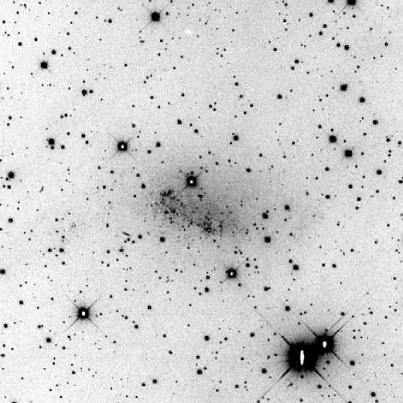
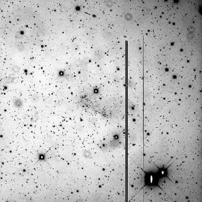
Figure 2: The dwarf galaxy EGB 0427 +63: One hour light on 0.8 m WST telescope, best seeing and lowest sky 20 images of four days stacked; left: image; right: error image.

6.5 Errors in convolution

We tested the accuracy of the convolution with 19 pairs of simulated frames: The reference frames with a FWHM of the stellar PSF of 2.4 and five times more flux than the comparison frames with a FWHM of 3.0, all with over 100 000 stars and different background levels. According to Sect. 5.2 the reference frames are convolved to match the PSF and the background level of the comparison frames. The convolved frames are subtracted from the comparison frames and the result divided by the expected RMS errors, as derived from error propagation. This gives the ratio of expected photon noise and measured noise. The histogram of such a ratio frame matches a Gaussian with $\sigma=1$ almost perfectly, which means that the expected photon noise fits the measured noise. This shows that the OIS method can be applied to very crowded fields like M 31 and gives residual errors at the photon noise level (Fig. 3).

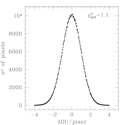
Figure 3: Histogram of the pixel values of a simulated difference image divided by the expected RMS errors. The solid curve is a Gaussian with $\sigma=1$. We calculate the reduced chi-square $\bar{\chi}^{2}$ of 19 different simulated images in the range between -3 and 3. The median is 1.1, which means that expected and measured errors match almost perfectly and that the residuals in the OIS are at the photon noise level.

6.6 Errors in interpolations – PSF-fitting photometry

We performed PSF-fitting photometry in simulated images as described in Sect. 5.5 using a Moffat fitting function (Eq. 48) on bright stars, and (together with OIS, using a high signal-to-noise reference image) on faint variable sources in a crowded and a highly crowded field. We found that per pixel propagated errors compared to estimated errors greatly enhanced the reliability of any fit. Extensive testing with simulated images comprising different observational features shows that this is especially due to the treatment of defective pixels, cosmics and saturation (pixel defects). If we want to avoid the labour of full error propagation we nevertheless have to use masks to get rid of these pixel defects. But then long time series will diminish our field, because the defects will spread (due to dithering, minor misspointing, different detectors, random position defects etc.). Furthermore, the $\bar{\chi}^{2}$ (Eq. 25) of a fit has a valid meaning only for fully propagated errors: $\bar{\chi}^{2}\approx 1$ implies a correct measurement within purely noise induced errors and correctly flagged pixel defects; $\bar{\chi}^{2}>1$ indicates systematic errors beyond noise and corrected pixel defects like blending of variable sources, missed or wrongly treated pixel defects. Renouncing full error propagation will shift e.g. bad flatfields from the recognised, high noise category to the undiscovered systematics regime. The calculated error will not change, because we consider $\bar{\chi}^{2}$ for the final error budget, but we would lose the chance to investigate those cases. If one cannot prove the origin of the uncertainties in a measurement, one can neither be sure of the measurement itself nor of the postulated accuracy.

7 Summary

We have presented a standard image reduction pipeline applicable to any CCD images, but with the intention to execute DIA, i.e. image convolution and relative photometry. We put a great emphasis on the importance of per pixel propagated errors. The necessity of building good flatfield calibration images and a way to obtain them was shown. We also presented a robust filtering technique for cosmic rays applicable to single, not too undersampled images. We discussed all image reduction issues of finding variable objects and measuring their variations in highly crowded fields: PSF matching by convolution of a reference image using the Alard & Lupton (1998) technique, construction of difference images, detection algorithm for variable sources, and relative photometry of variable sources by a profile fitting technique.

A paper about the application of this image reduction pipeline on a massive imaging campaign of a part of the M 31 Bulge is accepted by A&A (Riffeser et al., 2001). Parts of the reduction pipeline have also been successfully applied to MUNICS data (cosmic-filtering of MOSCA spectra and CAFOS images; Drory et al., 2001) and VLT FORS data (cosmic-filtering and image alignment of revised FDF frames, A. Gabasch, priv. comm.; image alignment and OIS in the centre part of NGC 4697 using a difference image built of narrow on-band and off-band line images, Méndez et al., 2001).