Magnetic activity in accretion disc boundary layers

Abstract

We use three dimensional magnetohydrodynamic simulations to study the structure of the boundary layer between an accretion disc and a non-rotating, unmagnetized star. Under the assumption that cooling is efficient, we obtain a narrow but highly variable transition region in which the radial velocity is only a small fraction of the sound speed. A large fraction of the energy dissipation occurs in high density gas adjacent to the hydrostatic stellar envelope, and may therefore be reprocessed and largely hidden from view of the observer. As suggested by Pringle (1989), the magnetic field energy in the boundary layer is strongly amplified by shear, and exceeds that in the disc by an order of magnitude. These fields may play a role in generating the magnetic activity, X-ray emission, and outflows in disc systems where the accretion rate is high enough to overwhelm the stellar magnetosphere.

1 Introduction

The boundary layer between an accretion disc and a slowly rotating star can emit up to one half of the total accretion luminosity (Lynden-Bell & Pringle 1974), and has long been implicated as a probable site of variability (Pringle 1977; Papaloizou & Stanley 1986; Kley & Papaloizou 1997; Bruch 2000; Kenyon et al. 2000). Accretion via a boundary layer is likely both in weakly magnetic cataclysmic variables and neutron stars, and in young protostars where the accretion rate is high enough to overwhelm the stellar magnetic field.

Two theoretical difficulties hamper study of boundary layer structure. First, the dissipation of large amounts of energy into a narrow annulus requires a two-dimensional treatment of the thermal structure and radiation physics. Recent calculations of the structure of boundary layers in neutron star (Popham & Sunyaev 2001) and protostellar (Kley & Lin 1996, 1999) accretion have accomplished this goal. Second, the shear and radial force balance in the boundary layer are qualitatively different to the Keplerian disc, making approximate treatments of the angular momentum transport (or viscosity) especially suspect. This aspect of the problem has been less extensively investigated, although it is known that the Shakura-Sunyaev $\alpha$ viscosity prescription (Shakura & Sunyaev 1973) needs to be modified to yield physically reasonable boundary layer solutions (Pringle 1977; Papaloizou & Stanley 1986; Popham & Narayan 1992).

This paper presents initial results from boundary layer calculations that dispense with approximate viscosity prescriptions. Instead, numerical simulations are used to directly resolve the physical processes that lead to angular momentum transport. In sufficiently well-ionized discs, which include the inner regions of protoplanetary discs (Gammie 1996), the most important process is probably turbulence driven by magnetorotational instabilities (Balbus & Hawley 1991). The nonlinear study of these instabilities requires three dimensional magnetohydrodynamic (MHD) simulations, which we use to model the boundary layer between a geometrically thin accretion disc and a non-rotating, unmagnetized star. We confirm some aspects of prior theoretical work, but also find evidence for two novel effects – magnetic activity from fields amplified in the boundary layer (Pringle 1989), and dissipation which is concentrated in relatively high density regions (Clarke & Edwards 1989).

2 Numerical methods

The ZEUS code (Stone & Norman 1992a, 1992b, Norman 2000) is used to solve the equations of ideal MHD. ZEUS is an explicit, Eulerian MHD code, which uses an artificial viscosity to capture shocks. With the simplifying assumption that the fluid is isothermal (physically, this amounts to assuming that cooling occurs more rapidly than the other time-scales in the problem), the equations to be solved are,

$${{\partial\rho}\over{\partial t}}+\nabla\cdot(\rho{\bf v}) = 0$$ (1)

$${{\partial{\bf S}}\over{\partial t}}+\nabla\cdot({\bf Sv}) = -\nabla P-\rho\nabla\Phi+{\bf J}\times{\bf B}$$ (2)

$${{\partial{\bf B}}\over{\partial t}} = \nabla\times({\bf v}\times{\bf B})$$ (3)

$$P = \rho c_{s}^{2},$$ (4)

where ${\bf S}=\rho{\bf v}$, $\Phi$ is the gravitational potential, and the remaining symbols have their usual meanings.

The boundary layer itself is narrow. However, a larger domain is needed to model magnetorotational instabilities in the disc, which determine the structure of magnetic fields advected into the boundary layer region. We simulate a wedge of disc in cylindrical co-ordinates $(z,r,\phi$), using uniform gridding in both the vertical and azimuthal directions. For the radial direction, a non-uniform grid is employed in which the radii of successive grid cells are related by,

$$r_{j+1}=(1+\delta)r_{j},$$ (5)

with $\delta$ a constant. This concentrates resolution in the inner region of the flow.

High resolution, especially in the radial direction, is essential. To simplify the problem further, we ignore the vertical component of gravity and consider a vertically unstratified disc. This is a fair first approximation to the dynamics of the flow near the disc midplane, though if very strong fields were to develop in the simulation we would have to worry that they were overestimated due to the neglect of buoyancy. In practice, such strong fields were not obtained.

The initial conditions for the simulation comprise a static, non-rotating and unmagnetized atmosphere, surrounded by a Keplerian disc with an approximately gaussian density profile. To ensure that the initial conditions represent an accurate numerical equilibrium, the disc plus atmosphere structure was evolved in one dimension for a long period until all transients had died out. The resulting density and velocity profile (differing slightly from the input model) was then transferred to three dimensions, and a seed magnetic field added to the disc to initiate magnetorotational instabilities. Local simulations suggest that provided the seed field is weak, the properties of the final turbulent state are not strongly dependent upon the initial field geometry (Hawley, Gammie & Balbus 1995, 1996). We use a vertical seed field in order to achieve the most rapid transition to turbulence, and adopt an initial ratio of the thermal to magnetic energy density of $\beta=5000$.

The boundary conditions are periodic in $z$ and $\phi$, reflecting at $r=r_{\rm in}$ ($v_{r}=B_{r}=0$), and set to outflow at $r=r_{\rm out}$. Outflow boundary conditions are achieved by setting all fluid variables in the boundary zones equal to those in the outermost active zone, together with the constraint that $v_{r}\geq 0$.

The sound speed is set such that the ratio of the sound speed to the Keplerian velocity at the radial location of the boundary layer is $\simeq 0.1$ (precisely, $c_{s}=0.1$, while $v_{K}=1$ at the inner edge of the grid). This means that radial pressure gradients are small compared to the gravitational force in the accretion disc outside the boundary layer. In a stratified disc, the low sound speed would correspond to a geometrically thin flow in which the relative scale height $h/r\approx c_{s}/v_{K}\ll 1$.

Resolution	r	z	$\Delta\phi$	$n_{r}$	$n_{z}$	$n_{\phi}$
Low	$1\leq r\leq 5$	$\pm 0.2$	$45^{\circ}$	180	36	48
Medium	$1\leq r\leq 5$	$\pm 0.2$	$45^{\circ}$	300	60	80
High	$1\leq r\leq 5$	$\pm 0.2$	$45^{\circ}$	480	60	90

Table 1: Summary of the computational domain and resolution of the boundary layer runs.

Table 1 lists the parameters of the three runs discussed in this paper, which vary only in the numerical resolution. The highest resolution run has $n_{r}=480$, which corresponds to $r_{j+1}/r_{j}=1.003$. The code time units are such that the period of a Keplerian orbit at the inner edge of the grid at $r=1$ is $P=2\pi$.

3 Results

Figure 1: Growth of the magnetic energy density in the radial field during the high resolution simulation, integrated over the computational volume. The units on the $y$ axis are arbitrary.

Radial magnetic field is generated from the initial vertical field by magnetic instabilities. Figure 1 shows the evolution of the energy density of this field component in the high resolution simulation, averaged over the simulation volume. An initial phase of rapid exponential growth is followed by a slower increase as instabilities in the inner disc saturate. Similar results are obtained in all three simulations, although saturation is reached marginally earlier in the higher resolution runs. Only data from the shaded region near the end of the simulation, when the magnetic fields in the disc have reached an approximate steady state, is used for analysis of the boundary layer structure.

Figure 2: Evolution of the disc density with time, averaged over $z$ and $\phi$. Results are shown from the medium resolution run at $t=50$ (solid line), $t=100$ (dotted line), $t=150$ (short dashes) and $t=200$ (long dashes). The initial ($t=0$) profile is identical to that shown at $t=50$. Note that the density at the inner edge of the grid is $\gg 10^{2}$ – the limits for this figure have been chosen to emphasize changes in the density near the boundary layer.

The magnetic fields, generated in the disc by the action of magnetic instabilities, lead to angular momentum transport. This results in a redistribution of the disc surface density, shown in Figure 2. As expected, the inner high density hydrostatic envelope remains static, while the centre of mass of gas in the disc moves inwards. This is qualitatively in agreement with the diffusive evolution of a viscous accretion disc (e.g. Pringle 1981). Over the time-scale of the simulation, there is a small but clear change in the surface density in response to angular momentum transport in the disc.

3.1 Boundary layer structure

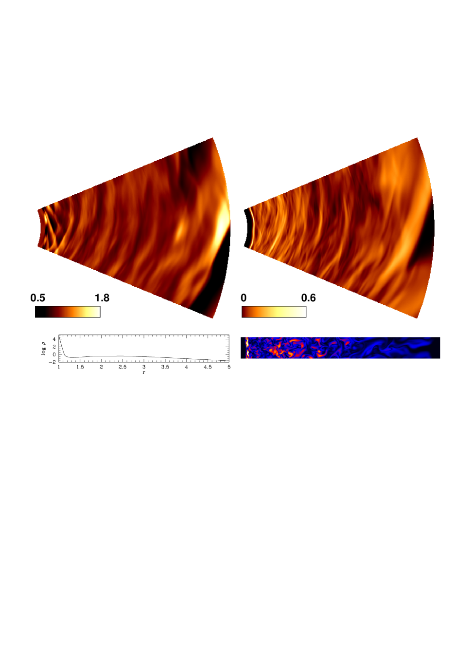
Figure 3: Results of the highest resolution run at $t=162.5$. Upper left panel: map of surface density fluctuations $\Sigma(r,\phi)/\Sigma(r)$. Typical fluctuations in $\Sigma$ are at the 10% level. Lower left panel: the mean density profile over the same radial range and at the same time. Upper right panel: the ratio of magnetic to thermal energy in the disc, averaged over $z$ in an $(r,\phi)$ map. Lower right panel: energy in magnetic fields (not normalized to the thermal energy) in a single $(r,z)$ slice. The strongest magnetic fields are typically found in the boundary layer. Averaged over $z$, they reach a peak of around 60% of the thermal energy at this timeslice.

Figure 3 shows images of the magnetic fields and surface density fluctuations in the simulation, at a time when the inner parts of the disc (roughly $r\ \raisebox{-1.29167pt}{$\stackrel{{\scriptstyle<}}{{\scriptstyle\sim}}$}\ 4$) are fully turbulent. The magnetic field in the disc is predominantly toroidal, with the strongest fields occupying a modest fraction of the simulation volume. The Keplerian angular velocity in the disc means that all structures are strongly sheared in azimuth. In this Figure, the boundary layer itself is visible as a narrow stripe in the magnetic field map, while interior to the boundary layer the gas remains in its initial quiescent, almost unmagnetized state.

Figure 4: Radial velocity $v_{r}$ and angular velocity $\Omega$ from the high resolution simulation, averaged over 5 timeslices between $t=150$ and $t=200$. The dashed curve in the lower panel shows a Keplerian profile for the angular velocity. Locations of mesh points have been plotted on the angular velocity curve to indicate the resolution achieved in the boundary layer region.

Figure 4 shows the mean radial and angular velocity, as a function of radius, in the disc and boundary layer. There are large temporal fluctuations, especially in $v_{r}$, so the plotted quantities are averaged over $z$, $\phi$, and over several approximately independent timeslices from near the end of the simulation. We plot results from the high resolution run, though for the radial velocity, angular velocity, and surface density, consistent results are obtained from all three simulations.

The structure of the boundary layer seen in the simulations agrees with expectations based on previous theoretical calculations. The angular velocity, which in the disc is very closely equal to the Keplerian value, makes a smooth transition over a narrow radial region to the stellar value. In the highest resolution run depicted, this boundary layer region is resolved across about 20 radial grid cells. The radial velocity exhibits larger fluctuations (even after averaging), and is actually largest just outside the boundary layer. The radial velocity remains highly subsonic, $v_{r}\ \raisebox{-1.29167pt}{$\stackrel{{\scriptstyle<}}{{\scriptstyle\sim}}$}\ 0.05c_{s}$, at all radii, as predicted using arguments based on causality (Pringle 1977; Popham & Narayan 1992).

3.2 Magnetic fields in the boundary layer

Figure 5: Strength of the magnetic fields in the flow. The upper panel shows the magnetic energy density as a function of radius in arbitrary units, the lower panel the ratio of the magnetic energy to the thermal energy. Results from the low (dotted line), medium (dashed line) and high resolution (solid line) runs are plotted, in each case averaged over several timeslices. The spike in magnetic energy at $r\simeq 1.15$ corresponds to the location of the boundary layer.

Figure 5 shows the magnetic energy density in the simulations, both in absolute terms and as a fraction of the thermal energy of the gas. In absolute terms, the strongest fields by far are obtained in the boundary layer. The magnetic energy density there exceeds that in the disc at larger radii by roughly an order of magnitude. This is an explicit demonstration of the amplification of magnetic fields by the strong shear in the boundary layer (Pringle 1989). It is also analagous to the situation inside the last stable orbit around black holes, where it has similarly been suggested that the presence of strong shear can amplify magnetic field energy relative to other energies in the system (Krolik 1999).

As a fraction of the thermal energy, there is a smaller but still pronounced spike in magnetic energy at the location of the boundary layer. We obtain magnetic field energies in the boundary layer that are between 10% and 20% of the thermal energy, compared to values in the disc of $\sim 5\%$ well away from the boundary layer region. Some individual timeslices – for example the one shown in Figure 3 – yield boundary layer fields that are substantially stronger still.

Unlike in the case of the radial and angular velocity, it is clear from Figure 5 that the magnetic field energy in the boundary layer has not converged at the highest resolution attained in the simulations (the magnetic fields in the disc, on the other hand, are consistent in the medium and high resolution runs). There is no clear trend with resolution, but the highest resolution run generates boundary layer fields that are substantially stronger than those in the medium resolution run. Since numerical reconnection at the grid scale is bound to artificially destroy magnetic fields, the conservative view is that the simulations demonstrate only that the boundary layer fields will be substantially stronger than those in the disc. Still stronger boundary layer fields, perhaps approaching or exceeding equipartition with the thermal energy (Pringle 1989), remain a possibility.

3.3 Dissipation

Figure 6: Location of the boundary layer. The region of the flow with ${\rm d}\Omega/{\rm d}r>0$ and $\Omega>\Omega_{*}$ (shaded region) corresponds to relatively high density gas adjacent to the outer part of the static atmosphere.

There is no energy equation, and hence no explicit dissipation, in these isothermal simulations. In a more realistic description, however, there would be a large accretion luminosity arising from dissipation of the rotational energy of the gas in or near the boundary layer region. It is therefore interesting to note that in the simulations, the boundary layer (defined here as the region where ${\rm d}\Omega/{\rm d}r>0$, and shown as the shaded band in Figure 6) lies in relatively high density gas that merges indistinguishably into the hydrostatic envelope that represents the star. This, of course, is only a restatement of the fact that angular momentum transport within the boundary layer is inefficient. As a result, the radial velocity in the boundary layer is very small – smaller in fact than in the disc immediately outside the boundary layer, and the density high. If these results hold also for more realistic boundary layers (which will be radially broader due to thermal effects), then they imply that a significant fraction of the boundary layer emission could be intercepted and reprocessed by the accreting object. The boundary layer luminosity would then be, at least partially, hidden from view of the observer.

4 Discussion

For computational reasons, and for the sake of simplicity, the simulations presented here assume that the accreting star is unmagnetized. This is not generally true, so we summarize here the conditions and systems for which it is a reasonable approximation.

The magnetic field of the accreting object, if it is strong enough, will disrupt the inner accretion disc and channel infalling matter along the field lines to the stellar surface (Pringle & Rees 1972; Miller & Stone 1997). Although the details are model dependent, the radius $r_{\rm m}$ at which the magnetic field will disrupt the disc is expected to be comparable to the spherical Alfven radius (Königl 1991),

$${r_{\rm m}\over r_{*}}=\beta_{\rm t}\left({{B_{*}^{4}r_{*}^{5}}\over{GM_{*}\dot{M}^{2}}}\right)^{1/7}.$$ (6)

Here $B_{*}$ is the surface magnetic field strength (assumed dipolar), and $\beta_{\rm t}$ is a scaling factor of the order of unity whose value depends upon the adopted model for the star-disc interaction (e.g. Ghosh & Lamb 1978; Shu et al. 1994).

Setting $r_{\rm m}/r_{*}=1$, and adopting magnetic field strengths and stellar radii appropriate for T Tauri stars (Guenther et al. 1999), the minimum accretion rate required to disrupt the disc is,

$$\dot{M}_{\rm crit}\simeq 2.5\times 10^{-6}\left({\beta_{\rm t}\over 0.5}\right)^{7/2}\left({M_{*}\over M_{\odot}}\right)^{-1/2}$$

$$\times\left({B_{*}\over{1\ {\rm kG}}}\right)^{2}\left({r_{*}\over{3r_{\odot}}}\right)^{5/2}\ M_{\odot}{\rm yr}^{-1}.$$ (7)

For a sample of classical T Tauri stars in the Taurus molecular cloud, Gullbring et al. (1998) estimated mass accretion rates in the range $10^{-9}\ M_{\odot}{\rm yr}^{-1}\ \raisebox{-1.29167pt}{$\stackrel{{\scriptstyle<}}{{\scriptstyle\sim}}$}\ \dot{M}\ \raisebox{-1.29167pt}{$\stackrel{{\scriptstyle<}}{{\scriptstyle\sim}}$}\ 10^{-7}\ M_{\odot}{\rm yr}^{-1}$. Accretion at these rates will result in the inner disc being disrupted by the stellar magnetosphere, rather than reaching the star and forming a boundary layer. Numerous observations support this conclusion (Najita et al. 2000).

In younger pre-main-sequence stars, however, the accretion rates are higher. At early times, the accretion rate through the disc is expected to be of the order of $c_{s}^{3}/G\sim 10^{-5}\ M_{\odot}{\rm yr}^{-1}$, where $c_{s}$ is here the sound speed in the collapsing cloud (e.g. Shu 1977; Basu 1998). Accretion rates of this order, along with (perhaps) weaker stellar fields, make boundary layer accretion more likely. Observationally, magnetic activity can certainly be present long before the optically visible Classical T Tauri stage. X-ray emission, indicative of powerful magnetic activity, is observed in some (though by no means all) of the youngest Class 0 and Class I sources (Feigelson & Montmerle 1999; Montmerle et al. 2000; Carkner, Kozak & Feigelson 1998; Tsuboi et al. 2001). Outflows, which provide less direct evidence of the presence of magnetic fields, are often powerful even in Class 0 sources (Bontemps et al. 1996). Boundary layers could play a role in some of these phenomena.

Identical arguments apply to white dwarf and neutron star accretion. Adopting parameters appropriate to a dwarf nova in outburst, the dipole magnetic field required to just disrupt the disc is,

$$B_{\rm crit}\simeq 10^{5}\left({\beta_{\rm t}\over 0.5}\right)^{-7/4}\left({M_{*}\over M_{\odot}}\right)^{1/4}\left({\dot{M}\over{10^{-8}\ M_{\odot}{\rm yr}^{-1}}}\right)^{1/2}$$

$$\times\left({r_{*}\over{5\times 10^{8}\ {\rm cm}}}\right)^{-5/4}\ {\rm G}.$$ (8)

This is not an enormous field, even though we have used an outburst accretion rate. In quiescence, typical accretion rates are much lower, and correspondingly weaker magnetic fields would suffice to disrupt the disc. Hence, in quiescent dwarf novae magnetic fields may well be strong enough to disrupt the inner accretion disc (Livio & Pringle 1992). Conversely, in supersoft X-ray sources (van den Heuvel et al. 1992), cataclysmic variables with higher accretion rates, and dwarf novae during outburst, boundary layers are likely to exist for relatively weakly magnetic white dwarfs. The results presented here suggest that emission from the boundary layer will be highly variable, but may be partially hidden from observational view.

5 Conclusions

In this paper, we have presented MHD simulations of the boundary layer between an accretion disc and a non-rotating, unmagnetized star. Although in these initial simulations drastic simplifications have been made in other aspects of the disc model, the inclusion of MHD allows us to resolve the physics underlying angular momentum transport in the disc and boundary layer region – one of the main areas of uncertainty in previous models. Three main results emerge from the simulations:

1. The basic structure of the boundary layer agrees with that predicted previously. The boundary layer is highly variable, narrow, and the radial velocity subsonic.

2. Magnetic fields generated in the disc are amplified by the shear in the boundary layer. Unless the star itself has a strong field, this means that the strongest magnetic fields in the star-disc system will be in the boundary layer. We derive magnetic energy densities that are a few tenths of the thermal energy. Resolution limitations mean that this is probably a lower limit to the true field strength.

3. Angular momentum transport in the boundary layer is inefficient, and as a result dissipation occurs primarily in relatively high density gas. Radiation originating from the boundary layer may therefore be partially ‘buried’ in the stellar envelope.

These results, if they apply also to boundary layers with more realistic thermal structures, suggest that in systems where boundary layers are present, they will be an important site of magnetic activity. Magnetic fields in the boundary layer could be important for producing the observed X-ray emission in these systems, and more speculatively could play a role in the formation of outflows.

References

- [1] Balbus S.A., Hawley J.F., 1991, ApJ, 376, 214
- [2] Basu S., 1998, ApJ, 509, 229
- [3] Bontemps S., Andre P., Terebey S., Cabrit S., 1996, A&A, 311, 858
- [4] Bruch A., 2000, A&A, 359, 998
- [5] Carkner L., Kozak J.A., Feigelson E.D., 1998, AJ, 116, 1933
- [6] Clarke C.J., Edwards D.A., 1989, MNRAS, 236, 289
- [7] Feigelson E.D., Montmerle T., 1999, ARA&A, 37, 363
- [8] Gammie C.F., 1996, ApJ, 457, 355
- [9] Ghosh P., Lamb F.K., 1978, ApJ, 223, 83
- [10] Guenther E.W., Lehmann H., Emerson J.P., Staude J., 1999, A&A, 341, 768
- [11] Gullbring E., Hartmann L., Briceno C., Calvet N., 1998, ApJ, 494, 323
- [12] Hawley J.F., Gammie C.F., Balbus S.A., 1995, ApJ, 440, 742
- [13] Hawley J.F., Gammie C.F., Balbus S.A., 1996, ApJ, 464, 690
- [14] Kenyon S.J., Kolotilov E.A., Ibragimov M.A., Mattei J.A., 2000, ApJ, 531, 1028
- [15] Kley W., Lin D.N.C., 1996, ApJ, 461, 933
- [16] Kley W., Lin D.N.C., 1999, ApJ, 518, 833
- [17] Kley W., Papaloizou J.C.B., 1997, MNRAS, 285, 239
- [18] Königl A., 1991, ApJ, 370, 39
- [19] Krolik J.H., 1999, ApJ, 515, L73
- [20] Livio M., Pringle J.E., 1992, MNRAS, 257, 15
- [21] Lynden-Bell D., Pringle J.E., 1974, MNRAS, 168, 603
- [22] Miller K.A, Stone J.M., 1997, ApJ, 489, 890
- [23] Montmerle T., Grosso N., Tsuboi Y., Koyama K., 2000, ApJ, 532, 1097
- [24] Najita J.R., Edwards S., Basri G., Carr J., 2000, in Protostars and Planets IV, eds V. Mannings, A.P. Boss & S.S. Russell, University of Arizona Press, Tuscon, p.457
- [25] Norman M.L., 2000, Rev. Mex. Astron. & Astrophys. (Conf. Ser.), 9, 66, astro-ph/0005109
- [26] Papaloizou J.C.B., Stanley G.Q.G., 1986, MNRAS, 220, 593
- [27] Popham R., Narayan R., 1992, ApJ, 394, 255
- [28] Popham R., Sunyaev R., 2001, ApJ, 547, 355
- [29] Pringle J.E., 1977, MNRAS, 178, 195
- [30] Pringle J.E., 1981, ARA&A, 19, 137
- [31] Pringle J.E., 1989, MNRAS, 236, 107
- [32] Pringle J.E., Rees M.J., 1972, A&A, 21, 1
- [33] Shakura N.I., Sunyaev R.A., 1973, A&A, 24, 337
- [34] Shu F.H., 1977, ApJ, 214, 488
- [35] Shu F., Najita J., Ostriker E., Wilkin F., Ruden S., Lizano S., 1994, ApJ, 429, 781
- [36] Stone J,M., Norman M.L., 1992a, ApJS, 80, 753
- [37] Stone J,M., Norman M.L., 1992b, ApJS, 80, 791
- [38] Tsuboi Y., Koyama K., Hamaguchi K., Tatematsu K., Sekimoto Y., Bally J., Reipurth B., 2001, ApJ, 554, 734
- [39] van den Heuvel E.P.J., Bhattacharya D., Nomoto K., Rappaport S.A., 1992, A&A, 97