A novel approach for extracting time-delays from lightcurves of lensed quasar images

We present a new method to estimate time delays from light curves of lensed quasars. The method is based on $\chi^{2}$ minimization between the data and a numerical model light curve. A linear variation can be included in order to correct for slow long-term microlensing effects in one of the lensed images. An iterative version of the method can be applied in order to correct for higher order microlensing effects. The method is tested on simulated light curves. When higher order microlensing effects are present the time delay is best constrained with the iterative method. Analysis of a published data set for the lensed double Q 0957+561 yields results in agreement with other published estimates.

1 Introduction

The time delay between light rays from gravitationally lensed quasar images is a measurable parameter directly related to the gravitational potential and to the Hubble constant $H_{0}$ (Refsdal Refsdal (1964)). Accurate time delays obtained from multiply lensed QSOs can hence be used i) to determine $H_{0}$ providing that the lens mass distribution is known, or ii) to constrain the mass distribution in a given lens, once $H_{0}$ has been determined from other methods (or other lensed QSO systems). Much effort has therefore been devoted to observations of lensed QSOs during the last years, and in particular to the photometric monitoring of lensed QSO images.

Measuring the time delay between the images of lensed quasars is, for several reasons, not a trivial task. First it requires regular monitoring of a target over a long period (substantially longer than the time delay). Second, the sampling is crucial and has to be determined on basis of the intrinsic variations in the quasar and the estimated time delay. Third, most objects are not observable during the whole year, i.e., they will be below the horizon for certain periods. Fourth, there are nights with bad weather conditions when no data are obtained. Finally, variations in lensed quasars may not only be due to intrinsic fluctuations of the quasar, but also to microlensing by compact objects along the line of sight. Such a microlensing signal, depending on its timescale and amplitude, can be used to constrain the size of the continuum and the line emitting regions in the quasar, and the distribution of compact matter in the lens galaxy (Paczyński  Pacz (1986), Kayser et al.  Kayser (1986)). However, as long as these external variations are not clearly distinguished from the intrinsic variations, microlensing remains a nuisance for time delay measurements. For the above reasons, advanced statistical methods have to be used to measure time delays from quasar light curves.

We have developed a method based on $\chi^{2}$ minimization of the data and a numerical model light curve. The aim was to develop a method based on simple principles, and to be able to properly detect and correct for possible microlensing effects. It has already been successfully applied to several time delay measurements (Burud et al. Burud (2000); Hjorth et al. Hjorth (2001)). In this paper we will present the principles of the algorithm (Sect. 2) apply it to various simulated light curves (Sect. 3) and to a public dataset of QSO 0957+561 from Serra-Ricart et al. (Serra-Ricart (1999)) (Sect. 4).

2 Method

Let us assume that we have light curves for two images, A and B, of a lensed quasar. There are N data points in each of the time dependent light curves $a(t)$ and $b(t)$ with measurement errors $\sigma_{a}$ and $\sigma_{b}$. The two curves are identical except for a shift in time, $\Delta t$, and in magnitude, $\Delta m$. It is therefore possible to model the two curves with one model curve $g(t)$, and the parameters representing the time delay and the magnitude shift. In some cases the light from one or both of the images may be microlensed by individual stars in the lensing galaxy. Except for the cases of high amplification events, which are of short duration, microlensing effects are often slow variations that can be modeled to first order as a linear variation with slope $\alpha$.

As model curve we choose an arbitrary curve with a fixed number of equally spaced sampling points, $M$. This model may be $\chi^{2}$ minimized to the two observed light curves. The minimization is done only for the N observed data points. In this way only the model curve is interpolated and not the data. We thus minimize the following function:

$${\cal F} = \sum_{i=1}^{N}\left[\frac{a(t_{i})-g(t_{i})}{\sigma_{a_{i}}}\right]^{2}$$ (1)

$$+\sum_{i=1}^{N}\left[\frac{(b(t_{i}-\Delta t)-(\Delta m+\alpha t_{i}))-g(t_{i})}{\sigma_{b_{i}}}\right]^{2}$$

The determination of the time delay from sampled light curves always relies on the implicit assumption that intrinsic variations are continuous in time and slow enough to be measured, given the adopted frequency of the observations. Consequently with this assumption, if the typical sampling interval is $\tau_{1}$, we can thus smooth the model curve $g(t)$ on the same time scale $\tau_{1}$ (e.g., typically 7 days when observations are obtained once per week). This is done by introducing a smoothing term which minimizes the square of the difference between the original model and the same model convolved with a Gaussian $r$ whose Full Width at Half Maximum (FWHM) is $\tau_{1}$. This smoothing is performed for all the points $M$ on the model curve $g(t)$ so that the dates without data points are smoothed out on the model curve and gaps in the observed light curves will not contribute significantly to the result. The smoothing term is multiplied by a Lagrange parameter $\lambda$. This parameter can be chosen so that the model curve matches the data correctly in a statistical sense (i.e., we get the correct $\chi^{2}$). In practice however, excessive smoothing will prevent the minimization from converging. Therefore the smoothest possible solution which allows the minimization to converge is usually adopted.

In a $\chi^{2}$ minimization it is assumed that all the data points are independent. However, a light curve often consists in groups of nearby points and more isolated points. In regions where the time sampling is much shorter than the intrinsic quasar variations, the different measurements do not really bring new information on the shape of the light curve. Rather, they increase the precision with which the quasar magnitude is known at that moment. They might even be affected by common systematic errors, i.e. coming from a microlensing variation with a time scale comparable to the interval covered by these neighbouring points.

In such cases of strongly uneven time coverage, we find that the best results are often obtained when a weight $W_{i}$ is given to each data point in the following manner. For a point at a time $t_{i}$ we calculate the relative distance $t_{i}-t_{j}$ to all the other points in the curve. A Gaussian function with a FWHM$=2\sqrt{2\ln(2)}\tau_{2}$ chosen by the user is centered at $t_{i}$. The inverse of the sum of the ordinates of the Gaussian for each of the points $t_{j}$ will give the weight for the point $t_{i}$. The expression of $W_{i}$ can be written:

$$W_{i}=\frac{1}{\sum_{j=1}^{N}exp{(-\frac{t_{i}-t_{j}}{\tau_{2}})^{2}}}$$ (2)

The weight is normalized so that the maximum allowed weight for a data point is $1$, and this will occur only when one point is present within the time interval defined by $\tau_{2}$. The ideal choice of $\tau_{2}$ is the approximate time scale of variations in the quasar. For some systems this time scale will be long, e.g., several hundred days, for other systems it can be shorter e.g., 50 days. We can now write the final function to be minimized:

$${\cal F} = \sum_{i=1}^{N}W_{i}\left[\frac{a(t_{i})-g(t_{i})}{\sigma_{a_{i}}}\right]^{2}$$ (3)

$$+\sum_{i=1}^{N}W_{i}\left[\frac{(b(t_{i}-\Delta t)-(\Delta m+\alpha t))-g(t_{i})}{\sigma_{b_{i}}}\right]^{2}$$

$$+\lambda\sum_{i=1}^{M}\left[g(t_{i})-\left[r*g\right](t_{i})\right]^{2}$$

where $r*g$ signifies a convolution between $r$ and $g$.

2.1 Microlensing effects and iterative version of the algorithm

Slow microlensing variations in one of the light curves are modeled as a linear term with the parameter $\alpha$. If higher order variations are present we can use the method in an iterative way. This is done by splitting the light curves into several parts and analyzing them separately. The $\chi^{2}$ method is applied to determine the amount of linear external variations ($\alpha$) for each separate part and for a range of input time delay values. First we run the programme with the first time delay $dt_{1}$ in the chosen range and we estimate $\alpha$ in each of the separate parts. We then correct each part with the corresponding $\alpha$ and add the parts back together in order to obtain a set of microlensing-corrected light curves for the given input time delay $dt_{1}$. We can now run the $\chi^{2}$ method to measure the time delay for these “corrected” curves. This procedure is repeated for all the input time delay values $dt_{2}$, $dt_{3}$, … $dt_{n}$ in the range to be studied. We finally obtain a time delay measurement for each of the $n$ input values, and all these measurements will generally converge towards the real time delay value.

3 Time delay measurement on simulated light curves

3.1 Data simulations

We apply the method to simulated light curves in order to understand and estimate the errors on the measured values. Various real quasar light curves were used as models for typical time variations and sampling of data points. The measurement errors in the curves represent simulated photon noise errors, so that the faint component will have larger errors than the bright one. We present the results from two sets of simulated light curves. The first set (1a, b and c in Table 1) consists of two curves, A and B, each of 60 points, dispersed over a time interval of 2 years (see Fig. 1 (top) and 2 (top)). The B curve is shifted by 145 days in time and has a magnitude offset of 1.95 mag. In set 1b we have added a slow linear time dependent variation with a slope $\alpha$ (Eq. 3) in the B curve in order to simulate long-time-scale microlensing effects (Fig. 1 middle). A higher order microlensing variation ($\alpha t+\beta t^{2}$) is added to the B curve in set 1c (Fig. 1 bottom). In the second set (2a, b, and c) we have simulated another kind of intrinsic variation and sampling. The curves span an interval of two years and they have 36 data points each. The time delay is 110 days and the magnitude offset is 0.67 mag (see Fig. 3 top). In sets 2b and c, we added linear (b) and higher order (c) variations in the A curve (see Fig. 3 middle and bottom).

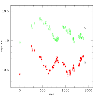
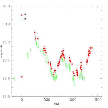
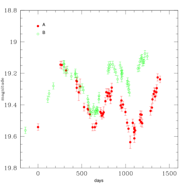
Figure 1: Top: The simulated light curves of two quasar components in set 1a (see text and Table 1). Middle: The time delay and magnitude shifted curves in set 1b. The remaining difference between the two curves corresponds to the linear microlensing variation. Bottom: The light curves in set 1c, shifted in time delay and magnitude. The remaining difference between the two curves is the higher order microlensing variation.

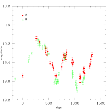
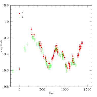
Figure 2: Top: The time delay and magnitude shifted light curves form set 1a. Bottom: The microlensing-corrected light curves derived by the iterative run on the curves in set 1c.

3.2 Time delay measurements

The $\chi^{2}$ algorithm was applied to all the simulated sets of light curves. The fit was performed several times in order to check for the influence of various parameters such as: (i) the number of data points in the model curve ($M$ in Eq. 3), (ii) the FWHM ($\tau$) of the Gaussian used to smooth the model curve ($r(t)$ in Eq. 3), (iii) the FWHM ($2\sqrt{2ln(2)}\tau_{2}$) of the Gaussian that defines the time scale of the variations in the curve (used to determine the weight $W_{i}$ in Eq. 3), and (iv) the Lagrange parameter ($\lambda$ in Eq. 3). For the first set the best results were obtained when including a weight ($W_{i}$ in Eq. 3) whereas for the second set the best results were obtained with no weight. This is because the data points in the second data set are more regularly distributed over time. The smoothing parameters were chosen so that the model curve is smooth over time, but still allowing variations large enough to fit the data. The results are shown in Table 1.

We performed Monte Carlo simulations to estimate the errors in the results. Sets of 1000 light curves were simulated with error bars determined randomly from a Gaussian distribution with a $\sigma$ equal to the measurement errors ($\sigma_{a}$ and $\sigma_{b}$). One set was made with the same sampling as the original curves (the simulated examples) and another set of 1000 curves was created with the same number of sampling points as the original, but randomly distributed.

When applying the iterative algorithm it is natural to think that the choice of the number of individual parts $n$ is important for the results. Various tests on our simulated curves indicate that if $n$ is too small, there is little difference from the total curve and higher order microlensing effects can not be properly corrected for. If on the other hand $n$ is too high, each part will contain very few data points and for some parts (depending on the sampling) the overlap between the two curves will be too small to determine the external variations. The choice of $n$ will thus depend on the number of data points and on how they are distributed (e.g., presence of gaps in the curves). The optimal values for the curves in the simulated curves, i.e., the values resulting in the best convergence of $\Delta t$, were found to be 3 and 2 in sets 1 and 2 respectively. The results shown in Table 1 correspond to the mean and standard deviation of the values obtained.

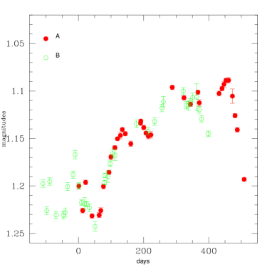
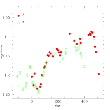
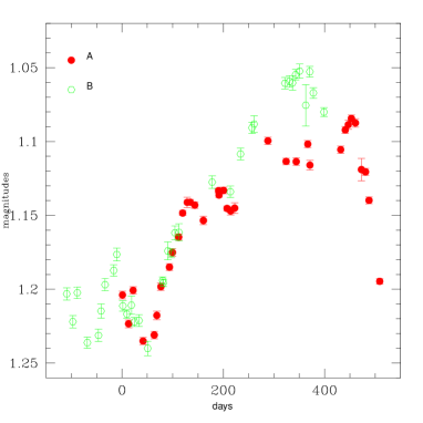
Figure 3: Top: The simulated light curves of two quasar components in set 2a (see text and Table 1). Middle: The time delay and magnitude shifted curves in set 2b. The remaining difference between the two curves corresponds to the linear microlensing variation. Bottom: The light curves in set 2c, shifted in time delay and magnitude. The remaining difference between the two curves is the higher order microlensing variation.

3.3 Results

All the time delay measurements obtained in sets 1a, b and 2a, b are very well determined within the estimated errors (see Table 1). As expected, the results depend on the sampling of the light curves and the error estimates from the Monte Carlo simulations with random sampling are larger than the ones obtained with a fixed sampling. In sets 1b and 2b where a slow linear variation is added in one of the curves, the time delay is still well determined whereas in sets 1c and 2c where higher order variations are added there are small systematic errors in the time delay estimated with the direct method. In these cases, the iterative method gives more accurate results with smaller uncertainties. Fig. 2 displays how the microlensing effects in data set 1c are corrected for with the iterative method. In the sets with no microlensing (1a and 2a) we note that the iterative method yields larger errors than the direct method. When no external variations (simulated microlensing effects) are present the best constrained time delay value is obtained by setting $\alpha=0$, hence removing one of the free parameters. The iterative method should therefore preferably only be applied where external variations are clearly present.

The magnitude shifts between the two curves are very well determined in sets 2a, b and c whereas in example 1a, b and c there are small systematic errors of $0.01-0.05$ mag.

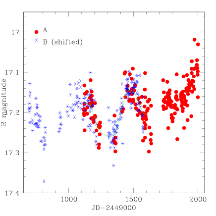
Figure 4: The R-band light curves of QSO 0957+561. The curve is shifted by 423 days and 0.0625 mag. The solid line shows the model curve derived by the $\chi^{2}$ algorithm.

Table 1: Results from the analysis of the simulated light curves. The sets (a, b and c) correspond to simulations with respectively no, linear and higher order external variations in one of the components. These variations simulate microlensing effects (see the text for more details).

light curves	1a	1b	1c	2a	2b	2c
true $\Delta t$	145	145	145	110	110	110
derived $\Delta t$:
direct method	143$\pm$5	151$\pm$5	132$\pm 5$	109$\pm$3	119$\pm$5	119$\pm$4
M.C. fixed sampling	146$\pm$5	148$\pm$5	135$\pm 5$	109$\pm$3	114$\pm$5	115$\pm$4
M.C. random sampling	155$\pm$23	149$\pm 16$	147$\pm$18	118$\pm$35	117$\pm$32	118$\pm$24
Iterative method	145$\pm$7	145$\pm 2$	143$\pm 9$	108$\pm$6	111$\pm$3	114$\pm$8
true $\Delta m$	1.950	1.950	1.950	0.670	0.670	0.670
derived $\Delta m$:
direct method	1.923$\pm$0.002	1.968$\pm$0.004	1.868$\pm 0.004$	0.667$\pm$0.001	0.667$\pm$0.003	0.647$\pm 0.004$
M.C. fixed sampling	1.927$\pm$0.002	1.964$\pm$0.004	1.885$\pm 0.004$	0.667$\pm$0.001	0.665$\pm$0.003	0.678$\pm 0.004$
M.C. random sampling	1.921$\pm$0.005	1.963$\pm$0.036	1.905$\pm$0.08	0.672$\pm$0.017	0.65$\pm$0.04	0.65$\pm$0.02
Iterative method	1.90$-$2.0	1.91$-$2.01	1.95$-$2.31	0.64$-$0.67	0.65$-$0.69	0.65$-$0.69

4 Application to light curves of QSO 0957+561

Our method was also applied to a public data set of QSO 0957+561 published by Serra-Ricart et al. (Serra-Ricart (1999)) (see Fig. 4). The R-band lightcurves contain 214 data points and span the time interval from February 1996 to July 1998. We removed eight points that deviate by more than 0.05 mag from neighbouring points in both components. We applied our $\chi^{2}$ algorithm to the data and, as was done for the simulated data, we estimated the error bars using Monte Carlo simulations. A time delay estimate $\Delta t=423\pm 9$ days and a magnitude shift $\Delta m=0.063\pm 0.007$ were obtained. Considering the two gaps in the data set, JD 2450242 to 2450347 and JD 2450637 to 2450729, Serra-Ricart et al. have divided the data set into two parts, DS I and DS II. Since the second part (DS II) show the largest activity they have determined a time delay value on DS II only, corresponding to the autumn 1997/spring 1998 season. They measure a time delay value of 425$\pm$4 days and a magnitude shift of 0.06 mag on these curves. Measurements with two other methods, the dispersion spectra and discrete cross-correlation techniques give values of $426\pm 12$ and $428\pm 8$ days respectively on the same data set (Serra-Ricart et al. 1999). In order to compare the results we therefore also apply our method to DS II. On the curves in DS II we measure $\Delta t=424\pm 22$. Both time delay values, the one measured on the entire data set and the one measured on DS II, are compatible with the results from Serra-Ricart et al. However our errors are larger than the ones found by Serra-Ricart et al. In particular we note that our errors are considerably larger when using only DS II than when using the entire data set. Serra-Ricart et al. do not give any time delay measurement from the total curve but their method seems to be well suited for time delay measurements on a continuous curve (DS II), even when the time span of observation is only of the order of the time delay value. With our method the time delay is better constrained with longer time series, even if gaps are present in the curves.

An additional reason for the differences in the results might be that whereas we have discarded 8 points form the total light curve, Serra-Ricart et al. have discarded 23 points. Given our limited knowledge of the data points we found no reason to exclude more points.

5 Conclusion

We have developed a method to determine time delays between light rays from lensed quasar images from their respective light curves. As other $\chi^{2}$ based methods (e.g., Press et al. Press (1992) and Barkanna Barkanna (1997)) we assume that the statistics of the measurement errors are Gaussian, and we require smoothness for nearby points in the light curves. In our method we have included an optional weight to each of the data points, depending on the relative distance to neighbouring points. In this way one point isolated in time will receive more weight than each individual point in a cluster of nearby points.

Since microlensing effects are often encountered in real light curves of lensed quasars we have adapted our method in order to correct for such variations. A linear term in one of the curves is included to correct for slow long-term variations. Realistic simulations show that the time delay and the magnitude shift between two light curves are determined to within a few percent for cases with no or slow microlensing effects. For faster microlensing variations we find that running the algorithm in an iterative way yields better time delays. This confirms what was proposed in the time delay measurement of B1600+434 (Burud et al. Burud (2000)) for which four methods were applied: the minimum dispersion method (Pelt Pelt (1996)), the SOLA method (Pijpers Pijpers94 (1994), Pijpers (1997) ), the method described in the present paper and its iterative version. The iterative method yielded the best constrained time delay in this data set due to external variations in one of the components.

We also applied our method to a public data set of QSO 0957+561 and have shown that our results are in agreement with the published time delay.

- (1) Barkanna, R., 1997, ApJ, 489, 21
- (2) Burud I., Hjorth J., Jaunsen A. O., et al., 2000 ApJ 544, 117
- (3) Hjorth, J., Burud, I., Jaunsen, A. O. et al., 2001, in Gravitational Lensing: Recent progress and future goals, ASP Conf. Ser., eds. T. Brainerd and C. Kochanek, in press
- (4) Kayser, R., Refsdal, S., Stabell, R. 1986, A&A, 93, 297
- (5) Paczyński, B., 1986, ApJ, 301, 503
- (6) Pelt, J., Kayser, R., Refsdal, S., Schramm, T. 1996, A&A, 305, 97
- (7) Pijpers, F. P., 1997, MNRAS, 289, 933
- (8) Pijpers, F. P. & Thomson, M. J., 1994, A&A, 281, 231
- (9) Press, W. H., Rybicki, G. B. & Hewitt, J. N. 1992, ApJ, 385, 404
- (10) Refsdal S. 1964, MNRAS, 128, 307
- (11) Serra-Ricart, M., Oscoz, A., Sanchís, et al., 1999, ApJ, 526, 40