The Magellanic Clouds Photometric Survey: The Small Magellanic Cloud Stellar Catalog and Extinction Map

Abstract

We present our catalog of $U$, $B$, $V$, and $I$ stellar photometry of the central $18{\rm\ sq.}^{\circ}$ area of the Small Magellanic Cloud. We combine our data with the 2MASS and DENIS catalogs to provide, when available, $U$ through $K_{S}$ data for stars. Internal and external astrometric and photometric tests using existing optical photometry ($U$, $B$, and $V$ from Massey’s bright star catalog; $B,V$, and $I$ from the microlensing database of OGLE and $I$ from the near-infrared sky survey DENIS) are used to determine the observational uncertainties and identify systematic errors. We fit stellar atmosphere models to the optical data to check the consistency of the photometry for individual stars across the passbands and to estimate the line-of-sight extinction. Finally, we use the estimated line-of-sight extinctions to produce an extinction map across the Small Magellanic Cloud and investigate the nature of extinction as a function of stellar population.

1 Introduction

The Magellanic Clouds, which are the largest nearby galaxies, provide our most detailed view of the extragalactic universe. Although their proximity is generally an advantage, their large angular extent on the sky has hampered global studies. Historically, stellar catalogs of the Clouds have relied on photographic data (see Hatzidimitriou et al. (1989) and Irwin et al. (1990) for some of the most recent examples). Within the last decade, several large-scale digital surveys of the Magellanic Clouds have been undertaken. In the optical bands, the principal ones are the microlensing surveys (MACHO, Alcock et al. (1997); OGLE, Udalski et al. (1998); and EROS, Palanque-Delabrouille et al. (1998)), an emission line survey (Smith et al. (2000)), a bright star survey (Massey (2001)), the red optical channel ($I$) of the infrared DENIS survey (Epchtein et al. (1997)), and our Magellanic Clouds Photometric Survey, hereafter MCPS (Zaritsky et al. (1997)).

We present the stellar photometric data in catalog form from the MCPS for the entire Small Magellanic Cloud (SMC) survey region (roughly $4.5^{\circ}\times 4^{\circ}$, where the longer direction is north-south). The principal advantages of these data in comparison to the surveys listed above are that our data are either deeper, cover a wider area, or include a larger number of filters (the inclusion of $U$ is particularly important for studies of dust and young stellar populations). However, as we show in our comparison to these other catalogs, each of the other surveys has its complementary strengths and we incorporate data from several of them to augment the MCPS catalog.

In addition to providing the catalog, we construct and analyze extinction maps of the SMC. As we demonstrated for a portion of the LMC (Zaritsky (1999)), the extinction properties in the Clouds are not only spatially variable, but depend on stellar population. Therefore, for many scientific purposes the catalog alone is insufficient, one must correct the observed magnitudes and colors for a complex extinction pattern. We describe the MCPS in §2, discuss detailed comparisons with previous data to assess the quality of the catalog in §3, use the photometry to generate extinction maps of the SMC for two different stellar populations in §4, and present the final catalog in §5.

2 The Data

The data come from the ongoing Magellanic Cloud Photometric Survey (Zaritsky et al. (1997)). Using the Las Campanas Swope telescope (1m) and the Great Circle Camera (Zaritsky et al. (1996)) with a 2K CCD, we obtained drift-scan images for both Magellanic Clouds in Johnson $U,B,V,$ and Gunn $I$. The effective exposure time is between 4 and 5 min for SMC scans and the pixel scale is 0.7 arcsec pixel^-1. Typical seeing is $\sim$1.5 arcsec and scans with seeing worse than $\sim$ 2.5 arcsec are not accepted. Magnitudes are placed on the Johnson-Kron-Cousins photometric system (Landolt 1983; 1992). Data from observing runs from November 1996 to December 1999 are included in this catalog. The data are reduced using a pipeline that utilizes DAOPHOT II (Stetson (1987)) and IRAF. Only stars with both $B$ and $V$ detections are included in the final catalog.

The pipeline for reducing individual scans is a fairly standard application of DAOPHOT. Each of the 24 scans ($\times$ 4 for the four filters), which are either 9500 or 11000 pixels long (depending on whether they are on the eastern or western side of the SMC survey region) and 2011 pixels wide, is divided into 9 by 2 or 11 by 2 subscans that are roughly 1100 by 1100 pixels, with an overlap of about 100 pixels between the subscans that enables us to compare the results from the independent photometric reductions. There are two sources of discrepancy in the photometry from subscans; differing and inconsistent PSF models and aperture corrections, and nonphotometric conditions. The latter is difficult to evaluate on a subscan basis because each subscan is smaller than the 2K CCD used for the observations, and so adjacent subscans are not independent of atmospheric variations. Comparing the photometry from adjacent scans, rather than subscans, enables us to check the observing conditions, which were judged by eye during the observing to be photometric almost entirely over the 4 years. These two classes of overlaps, subscan and scan, provide complementary internal checks.

The result of the reduction pipeline is a catalog of instrumental photometry for each detected star in each filter and its right ascension and declination. The astrometric solution is derived from a comparison to stars in the Magellanic Catalogue of Stars (MACS; Tucholke et al. (1996)), whose coordinates are on the FK5 system. Solutions are reviewed and iterated if either the number of stars in the solution is less than 20 over the $\sim$ 12 arcmin $\times 12$ arcmin subscan, or the rms positional scatter of the matched stars is larger than 0.5 arcsec. There are only ten subscans for which we were unable to reduce the positional scatter below 0.5 arcsec (and these have rms $<$ 0.6 arcsec), while the median rms is 0.3 arcsec.

The instrumental magnitudes of stars in different filters are matched using a positional match that associates the nearest star on the sky within an aperture that is 3 times either the positional rms of that subscan or 1.2 arcsec, whichever is larger. The $V$ frame is used as the reference and only stars that have a match in the $B$ frame are retained for the final catalog. In crowded areas it is possible that the “nearest” star in one filter is not the correct match to the $V$ reference because of the uncertainties in the astrometric solution. We see some evidence of this problem when comparing to other data and when fitting atmospheric models (stars with highly anomalous colors), but except near the faint limit of the catalog or in extremely crowded regions this issue appears to be a minor problem. It is evident that one could invest more effort in attempting to make “correct” matches, but the quality of the photometry in regions where multiple stars are within $\sim$ 1 arcsec of each other in images with typical 1.5 arcsec seeing is strongly compromised in any case. In all cases we accept the closest match. Unlike errors in the photometric calibration, these errors can be estimated reliably using artificial star simulations.

To place each subscan on a self-consistent photometric system, we use the overlap region (these typically contain several hundred stars in common in $B$, $V$, and $I$ and several tens in $U$) to measure photometric differences. Each subscan has either two (if at the front or back edge of a scan) or three neighboring subscans within its scan and one more in the adjacent scan, unless the subscan is at the edge of the survey region. We calculate the median photometric shift of each subscan relative to its neighbors and we find the subscan with the largest offset. The photometry of that subscan is adjusted by the offset and the process is repeated until all subscans with a median offset that is greater than 0.02 magnitudes are corrected. This process converges quickly because of the use of medians rather than means. The subscans are then combined to produce a photometric catalog for each scan. A stellar density map, constructed from the resulting catalog, is visually inspected for areas that correspond to scan or subscan regions that are of anomalously high or low density relative to their neighbors. The photometry is adjusted interactively in these cases to correct the handful of clearly anomalous subscans or scans. This method only addresses anomalies that are $>$ 0.05 mag. Although we are concerned that this procedure could lead to systematic drifts from the correct zeropoints, our photometry is extensively tested by comparison to external data sets (see §3.2).

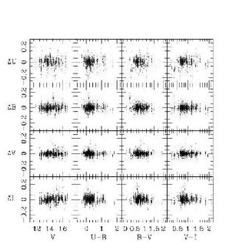
Figure 1: Standard star residuals from the mean photometric solutions. Each point represents the measurement for one standard star sometime during the 4 years of observations. The photometric solutions are independent for each observing run, but the same throughout a run.

The instrumental magnitudes are placed on the Johnson-Kron-Cousins Landolt system (1983; 1992). Residuals for the standard stars from our photometric solution are shown in Figure 1 over the four year period of the observing program. The photometric solutions involve a zeropoint term, an airmass term, and one linear color term (using $B-V$ for $B$ and $V$ and $V-I$ for $I$) or two linear color terms ($U-B$ and $B-V$ separately for $U$). Over the color range covered by the standards (see Figure 1) there is little evidence for additional color terms. The statistical zeropoint uncertainty is typically 0.02 mag per run, slightly higher in the $U$ band (0.03 to 0.04 mag) with only one run having a $U$ band uncertainty as high as 0.047 mag.

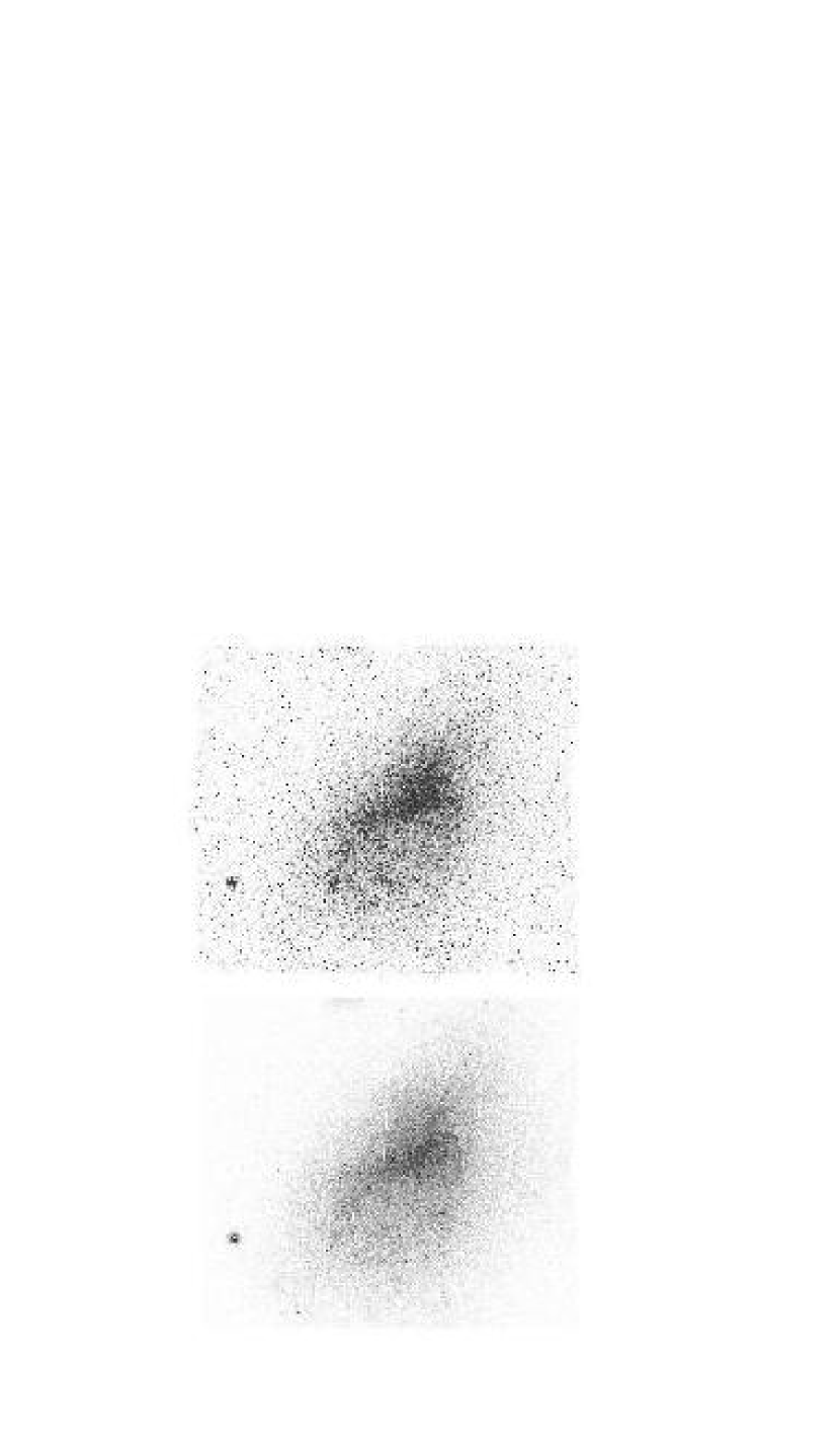
Figure 2: Grey scale representations of the SMC. The lower panel is a stellar number density map of stars with $V\leq 20$. The upper panel is a stellar luminosity density map of stars with $14<V<20$. North is left and East is to the bottom. The image shows the entire $\sim 4.5^{\circ}\times 4^{\circ}$ survey region. The nearly-horizontal white lines are caused by slight gaps between scans, which occurred if either the $V$ or $B$ scan was slightly misaligned. The large circular concentration of stars in the northeast is a Galactic globular cluster (NGC 362). The faint structure at the extreme western edge of the image is 47 Tuc.

The catalog of astrometry and photometry for 5,156,057 stars is presented as an ASCII table (see Table 1 for a sample). Columns 1 and 2 contain the right ascension and declination (J2000.0) for each star. Columns 3-10 contain the pairings of magnitudes and uncertainties for $U$, $B$, $V$, and $I$ magnitudes. The subsequent columns are described in §5. $V$ band stellar density and luminosity maps of the SMC are constructed from the catalog using stars with $V<20$ and shown in Figure 2. The digital catalogs allow one to make analogous images for a variety of populations (for other examples see the maps of young stars and evolved stars by Zaritsky et al. (2000)).

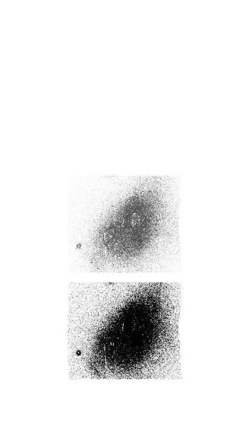
Figure 3: The stellar density map using stars with $20\leq V\leq 21$. The two panels show the same map at different contrast levels. Incompleteness, due to differing sensitivity limits caused either by sky brightness, seeing, or instrumental PSF variations from scan to scan are revealed by sharp discontinuities in the image. In the upper panel, the discontinuities between densities in different scans is evident in the central four scans, as is the drop in density where the SMC is in fact most crowded. At lower density levels (the outer isophotes in the lower panel) there are no obvious discontinuities at scan edges.

The magnitude limit of the survey varies as a function of stellar crowding. We find little visible evidence for incompleteness for $V<20$ (Figure 2), but the scan edges become visible when plotting the stellar surface density for stars with $20<V<21$ (Figure 3). Because of different sky brightness levels, seeing, and transparency, any completeness variations will be most noticeable at scan boundaries. We conclude that the stellar density differences are due to image quality (and the ability to resolve crowded stars), rather than either to variable sky brightness or transparency, because the scans have the larger density differences in the inner, crowded regions. In particular, the densities of the central four scans differ by a factor of 30% in the worst central areas for this range of magnitudes. In contrast, the outer isophotes, even at these magnitudes, are uniform across scan edges (Figure 3). The $U$ and $I$ data are incomplete at brighter magnitudes than the $B$ and $V$ data. The $U$ and $I$ photometry, even in sparse areas, is severely incomplete below $U=21.5$ and $I=22$ (comparable limits in the two other bands are $B=23.5$ and $V=23$). Any statistical analysis of this catalog fainter than $V<20$ requires artificial star tests to determine incompleteness, which is becoming significant at these magnitudes.

3 Testing the Photometry

3.1 Internal Tests

The overlap regions between subscans provide an indication of the internal reliability of the photometry. Because subscan comparisons use the same image, they reveal the variation in photometry due to the different point-spread function (PSF) models and aperture corrections used for the analysis of each subscan. Although the true PSF of the overlap stars is obviously the same in both subscans (since they come from the same original scan) the PSF models can vary among subscans due both to atmospheric effects and mechanical effects (for example, small misalignments or position errors that are corrected in subsequent moves of the camera) that are not the same over the entire subscan for each of the overlapping subscans. Partially, the initial motivation for dividing the scans into 1K subscans was that PSF variations appear manageable across individual subscans of this size. Although variations are visible even in these smaller regions, the DAOPHOT PSF is allowed to vary across the image, and the residuals after subtracting the fitted stars was deemed acceptable. With our internal and external tests we will determine the extent to which this conclusion is correct.

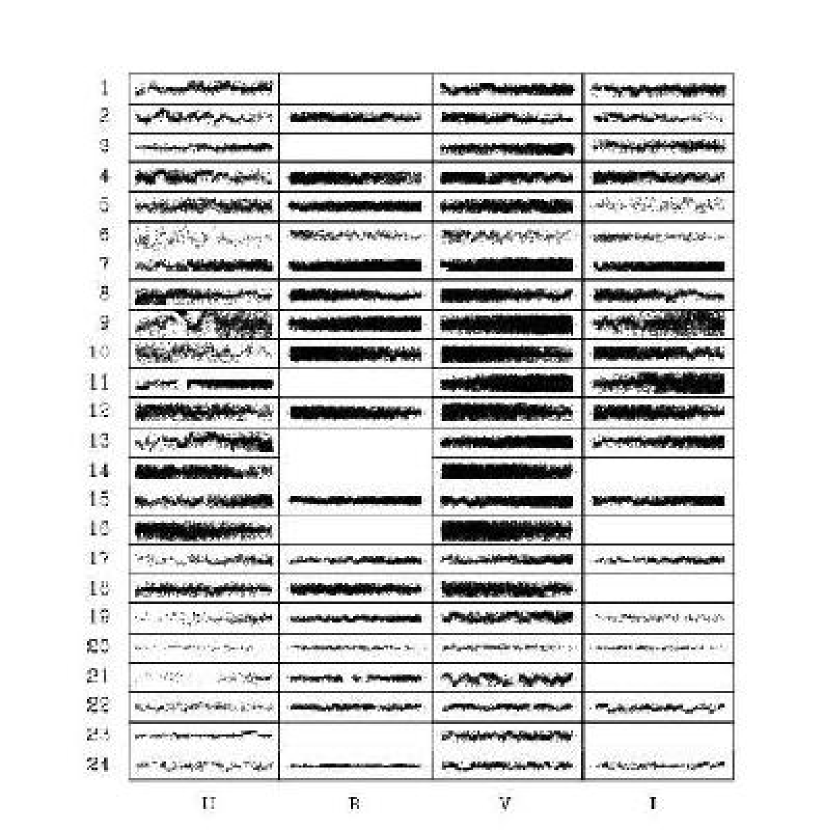
Figure 4: Photometry comparison of one half of a scan vs. the other half. Each point represents one star in common. The numbers to the left indicate the scan numbers (scan 1 is at the southwest, scan 2 is at the southeast and the scan numbers increase northward). The filters are labeled at the bottom. In all panels the vertical axis is $-0.2$ to 0.2 mag and the horizontal axis includes the entire scan. Empty panels indicate scan/filter combination for which there was no overlap due to slight misalignment of the scans. Only stars within 3$\sigma$ of the mean are included in the comparison, which in highly populated panels leads to sharp horizontal boundaries for the stellar locus.

Our first internal photometric test is provided by the overlap stars between one half of a scan and the other. We combine all of the subscans along each side of the scan and then compare the photometry in the overlap region. Again, because we are comparing the photometry for the very same stars within the same images, we are directly testing PSF model variations. Although apparently direct, this test is conservative in the sense that we are testing the PSF models for stars at the very edges of the frames, where the PSF models are most poorly constrained. The differences in stellar photometry across all of the scans where such overlap photometry is available are shown in Figure 4. In a few cases, the overlap region is unavailable because a scan in a particular passband is offset sufficiently from the $V$ band scan that the overlap region, defined in the $V$ frame, does not contain duplicate photometry in the other filter.

Excursions in the photometry residuals shown in Figure 4 come in two types: 1) a smoothly varying fluctuation (see scan 19 in $V$) and 2) a discontinuous jump (see middle of scan 4 in $U$). The first type of variation is due to PSF modeling variations. The PSF model is tracking real PSF variations, which are smoothly varying, differently in the two subscans, resulting in smooth differences in the photometry. The second type of variation is due to differences in the aperture corrections applied to the two different subscans. Initially, we attempted to correct for clear offsets such as that seen for scan 4 in $U$. However, we found that these applied offsets tended to make the photometry in the entire subscan worse. We conclude that there are PSF variations in the subscan that are not well-modeled near the edge, but that the aperture correction, which is calculated from stars throughout the subscan, is correct on average, but incorrect at the edge of the scan in some cases. This subtlety illustrates how Figure 4 provides an exaggerated view of photometric difficulties due to our focus on the edges of the scans. Even so, the photometric differences are typically small (the median of the rms deviations between different scan halves are 0.032, 0.015, 0.030, 0.028 mag for $U,B,V$ and $I$, respectively). The rms deviation is $<$ 0.05 mag in both $B$ and $V$ for all scans, and is $>$ 0.05 mag for only four $U$ and $I$ scans.

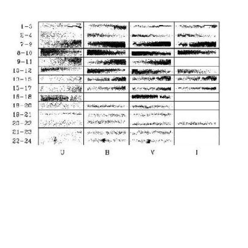
Figure 5: Photometry comparison of overlapping scans. Each dot represents one star in common. The numbers to the left indicate the scan pair, the filters are labeled at the bottom. In all panels the vertical axis is $-0.2$ to 0.2 mag and the horizontal axis includes the entire overlap region.

Our second internal test consists of examining the overlap regions between different scans. In this case, the images are taken under entirely different conditions, often in different years with different detectors. This test provides as good a test of the overall photometric accuracy as can be obtained internally. The magnitude differences along scans are shown for the four filters in Figure 5. Scan pairs come in E-W pairs and have the greatest overlap with scans in the N-S directions. Therefore, scans 1 and 3 overlap along a length of a scan, and scans 2 and 4 overlap. Some scan pairs that should overlap, such as 5 and 7, do not overlap because of a slight telescope offset in at least one filter (the gap between some scan pairs is visible in Figure 2. Again, these plots tend to exaggerate problems because we are examining the edges of scans, where the PSF’s are most likely to be distorted due to camera misalignments and tracking errors (as well as the poorly constrained PSF models). The photometric differences are evidently larger than in the comparison of scan halves because this comparison is based on different images of the same stars. The scatter is greater than before, but there are also some continuous variations (see the $U$ band comparison of scans 10 and 12). Even so, the median rms differences among the scans (comparing all overlap stars with $V<20$) are 0.13, 0.07, 0.06, and 0.05 mag for $U$, $B$, $V$, and $I$, respectively, These values are comparable or smaller than the quoted uncertainties for $V\sim 20$ stars, which dominate the comparison. We conclude that to the limit of the data, we have achieved a stable and robust photometric system across the survey.

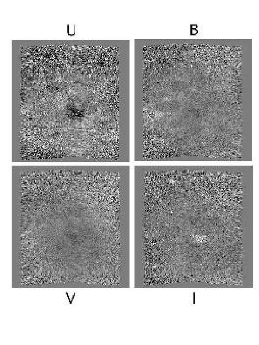
Figure 6: The local median of the red clump magnitude relative to the global value vs. position across the survey area. The four frames represent the results from each of the four filters, as labeled. The greyscales range from $-0.3$ to 0.3 magnitude and all images have a border beyond the survey area that is set to the global median, zero.

Our third internal test consists of using the red clump magnitude to examine spatial variations in photometry. We calculate the red clump mean magnitude in 70 $\times$ 70 arcsec boxes using stars that have $0.6<B-V<1.05$ and $18.8<V<19.8$. Although large-scale variations in the mean magnitude may truly exists (for example due to a tilt of the SMC relative to a constant-distance surface; see van der Marel (2001) for a demonstration of an analogous effects in the LMC), any localized variation, in particular one that traces scan or subscan boundaries, reveals a problem region. In Figure 6 we show the maps of the residual in the mean red clump magnitude relative to the global average, for all filters. There are various important features in these panels. First, all four panels show increased noise toward the edges because there are fewer clump stars at large radii from the SMC and contamination for foreground Galactic stars is proportionally greater. Second, the $U$ and $I$ band frames in particular show a suspicious feature just to the southwest of center. This is the most crowded region in the survey and we suspect that crowding has caused problems for the $U$ and $I$ photometry, which is not as deep as $B$ and $V$. The $B$ and $V$ photometry does not appear to have serious problems in this region at the magnitude of the red clump stars. The variations seen in the mid-left region of $B$ and in the center of the $V$ frame correspond to less than $\pm 0.05$ mags. Because these variations are more irregular (i.e. they do not follow the vertical or horizontal scan and subscan boundaries) we cannot determine whether these are real (for example, due to extinction variations) or due to photometric errors.

In conclusion, our internal tests suggest that there are photometric uncertainties of the order of a few hundreths of a magnitude between subscans and scans due to a combination of PSF modeling errors and calibration uncertainties. With the exception of potential crowding errors in $U$ and $I$ in the densest region of the SMC, the catalog appears to be limited by these uncertainties and Poisson noise down to at least $V\sim 20$.

3.2 External Tests

We are fortunate to have an array of existing data over substantial portions of the SMC with which we can further test the photometry in all four filter bands.

3.2.1 Comparison to Massey’s Catalog

Massey (2001) has produced a catalog of SMC photometry ($U,B,V$ and $R$) for bright stars along the central ridge of the SMC and toward the SMC wing. In particular, because of his interest in the upper main sequence, he pays particular attention to obtaining accurate $U$-band photometry for young SMC stars, which is often difficult because of the lack of blue ($U-B<0.0$) standards. We discuss various comparisons between that catalog and ours.

Astrometric Accuracy

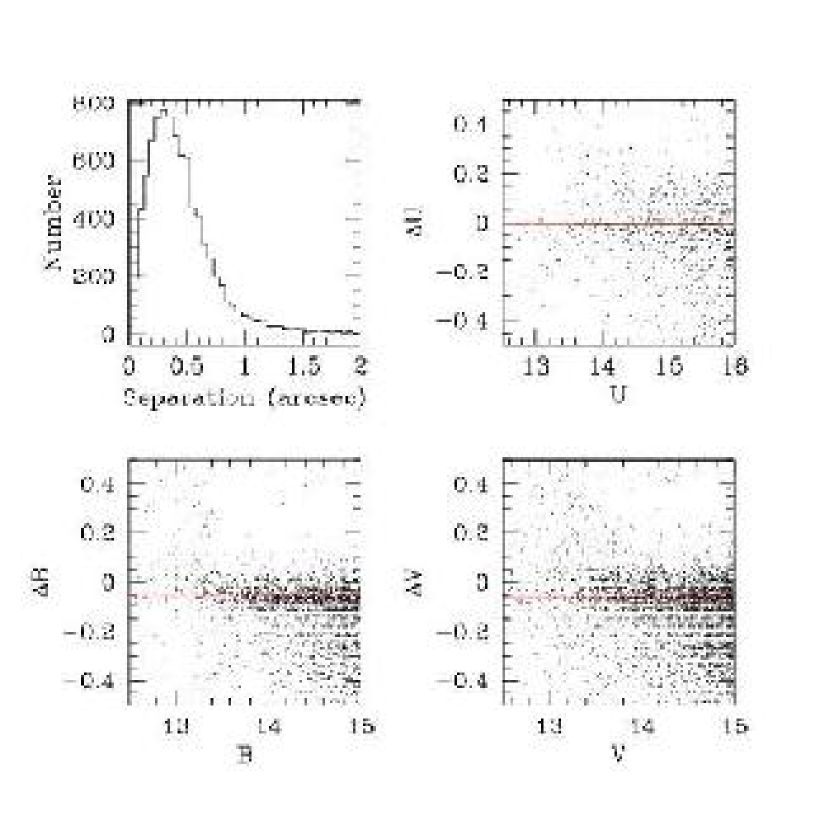
Figure 7: The comparison of the UBV photometry from our survey with that from Massey’s (2001) bright star survey. The upper left panel shows the distribution of matching separations between stars in the two surveys. The other three panels show the comparison of magnitudes with a horizontal line illustrating the mean difference over the range of magnitudes for which neither saturation nor confusion are a significant problem in either survey.

We match stars brighter than $V=15$ in Massey’s catalog to stars in the MCPS by finding the star in the MCPS within 7.5 arcsec of each Massey star that has the closest $V$ magnitude. The large search radius and the addition of the magnitude criteria has the potential to bias us away from picking the nearest star in projection. However, the distribution of separations (Figure 7, upper left) shows a strong peak toward matches with an offset that is $<1$ arcsec (the distribution peaks at $\sim 0.3$ arcsec). Although all matched stars are included in Figure 7, the offsets for stars with $V<13.5$ are somewhat larger and the reason for this is discussed in below. The astrometric correspondence between these two catalogs is excellent – certainly sufficient for spectroscopic follow-up of these stars.

Photometric Zeropoint Comparison

In Figure 7 we plot $\Delta m$ vs. $m$ for matched stars in $U,B,$ and $V$, where $\Delta m$ is defined to be Massey’s magnitude minus the MCPS magnitude. The bulk of the stars lie in a broad horizontal locus in these plots, with a flaring at $V<13.5$ toward positive residuals, and a flaring at $V>14.5$, toward negative residuals. Limiting the comparison to stars with positional offsets $\leq 0.7$ arcsec and $0.35<B-V$ for the $U$-band panel (see below for discussion of the color cut) and $13.5<V<14.5$ for $B$ and $V$ (eliminating the brighter magnitudes, where the MCPS has problems, and fainter magnitudes, where Massey’s data appear to have problems; see below) we calculate the mean offsets relative to $\Delta m$ = 0 to be $-0.057$ (after correction, see below), $-0.063,$ and $-0.057$ mag for $U,B,$ and $V$ respectively. These offsets are consistent with the photometric zeropoint errors of the studies, although slightly larger than expected. Fortunately, the colors, which are more sensitive to photometric zeropoint errors, are consistent between the two studies. We suspect that the systematic trend to negative mean residuals is at least in part due to the flaring toward negative residuals for individual stars at fainter magnitude, rather than a true photometric zero point difference. This flaring, as we show below, is due to crowding. An important consideration in this comparison, especially at the faint end, is that Massey’s magnitudes are aperture magnitudes within a large (8.1 arcsec) aperture.

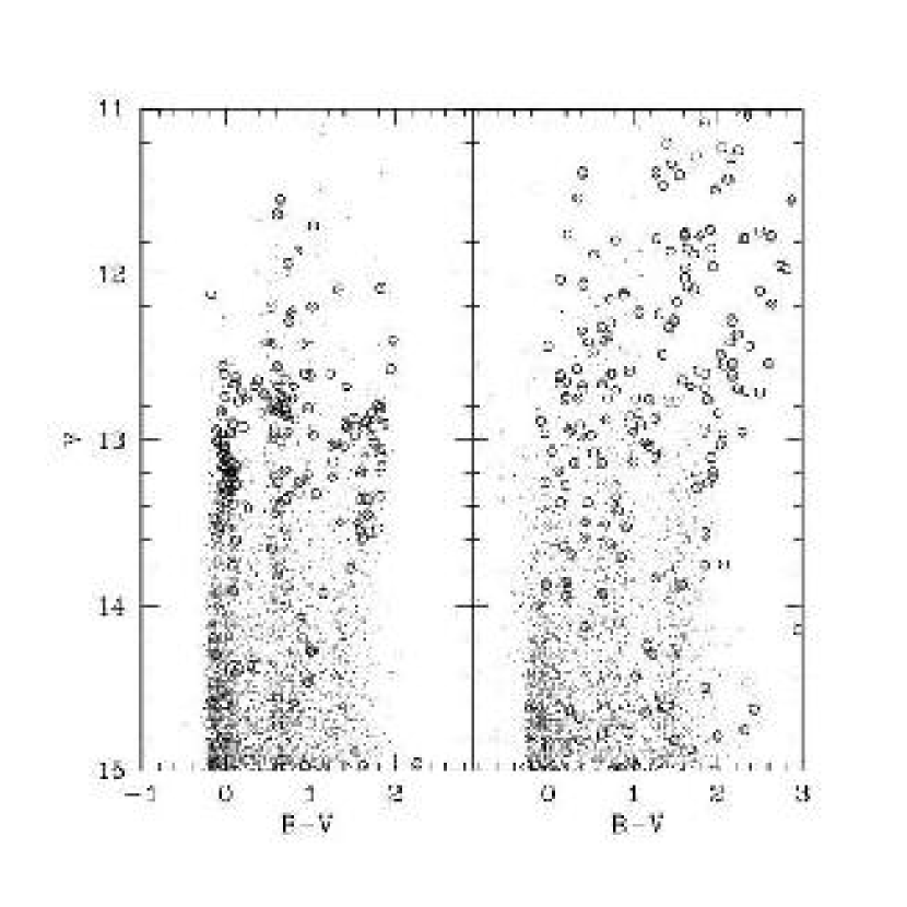
Figure 8: The bright star color-magnitude diagram using the data from Massey’s catalog on the left and from the MCPS on the right, for stars that have been matched between the two surveys. The open circles represent stars with $\Delta V>0.2$ mag and positional discrepancies $<$ 0.7 arcsec.

As already mentioned, in addition to the zeropoint offset of the horizontal locus, other features are visible in these diagrams. First, there is a diagonal flaring toward the upper left in the $B$ and $V$ panels of Figure 7. These are stars from the Massey (2001) catalog that are matched to a “brighter” star in our catalog. Because this problem appears only at bright magnitudes, we suspect it is due to poor PSF fitting of bright stars in the MCPS. In Figure 8 we show the color-magnitude diagrams for $B-V,V$ and highlight the stars with $\Delta V>0.2$ for both Massey’s catalog and the MCPS. It is evident from the tightness of the upper main sequence and red supergiant envelope for these stars that Massey’s photometry is superior at these bright magnitudes (the sequence visible between the main sequence and supergiants in the left panel are the foreground dwarfs). We conclude that stars in our catalog that are brighter than 13.5 in $B$ or $V$ are prone to substantial photometric uncertainty. Therefore, we have replaced the photometry and astrometry in our catalog for stars brighter than this limit with that of Massey (2001). In replacing our photometry with Massey’s, we apply the mean photometric offsets found between the MCPS and Massey’s catalog to Massey’s data. Because Massey’s catalog does not cover the entire area of our survey, not every star in the MCPS with $B,V<13.5$ has corrected photometry. To indicate which stars do have corrected photometry the catalog includes a flag (see §5 for a discussion of all of the quality flags). 809 stars are affected by this correction.

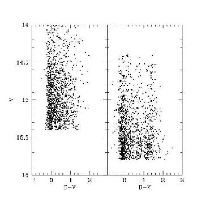
Figure 9: The color-magnitude diagram of fainter stars in common between the Massey survey on the left and the MCPS on the right that have $\Delta V<-0.3$ mag (the faint tail). The vertical (magnitude) offset between the stars in the two panels arises because we only include stars with $\Delta V<-0.3$.

The second systematic feature in these diagrams is the asymmetric distribution of $\Delta m$ toward fainter magnitudes. In this case, stars from the Massey (2001) catalog have been matched to fainter stars in the MCPS. Such a mismatch could occur if Massey’s catalog is beginning to be susceptible to unresolved blending, which is likely given the 8.1 arcsec aperture used for the aperture photometry. By comparing color-magnitude diagrams of stars with residuals $\leq-0.3$ (Figure 9), we find that in contrast to the situation with positive $\Delta m$, our data produce sharper main sequence and red envelope sequences. We conclude that at the faint magnitude limit of the comparison range our data are superior.

Photometric Color Term Comparison

In addition to zeropoint discrepancies, we use the Massey’s catalog to check for incorrect or missing color terms in our photometric solution. This issue is particularly important for the $U$ band because there are few blue calibration stars available in the standard fields. Massey (2001) has taken particular care to include a significant number of blue upper main sequence stars in the calibration, so we have reason to believe that his calibration in this regime is superior to ours.

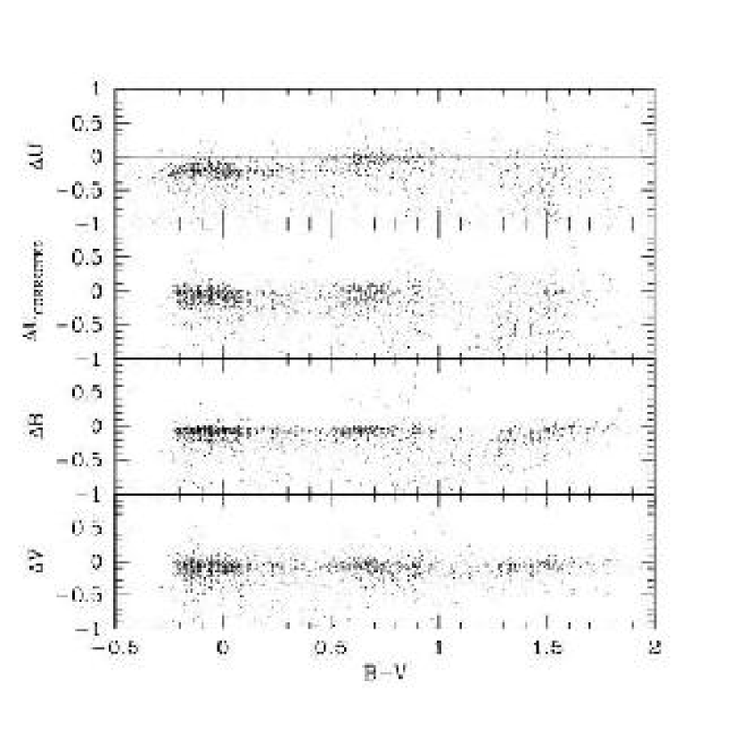
Figure 10: The comparison of magnitudes as a function of stellar color between the Massey survey and the MCPS. The upper panel shows the results from the original $U$ band photometry, the second panel shows the corrected $U$ band photometry.

The comparison of magnitudes for matched stars as a function of their $B-V$ color is shown in Figure 10. There are no grossly discrepant color terms in the $B$ and $V$ photometry, but the $U$ band photometry shows a noticeable shift ($\sim 0.2$ mag) the bluer and redder stars. Because we do not know whether the discrepancy lies in the bluer or redder stars, we apply the simplest (linear) correction to the $U$ band magnitudes that resolves this problem and minimizes the color differences between the MCPS and Massey’s catalog. This correction involves increasing the magnitudes by 0.05 mag for stars with $0.4<B-V<1.0$ and decreasing them by 0.05 mag for stars with $0.4>B-V$. We show the corrected photometry in Figure 10. The only other potential missing color term is suggested by a feature in the $B$-band photometry at $B-V\sim 1.1$ to 1.3. This is a sufficiently sharp feature (the $B$-band photometry returns to $\Delta m=0$ for $B-V>1.4$) that we do not correct for it and suspect that it is the result of beating between a slight difference in the filter transmission curve of the two studies and a spectral absorption feature in stars of this surface temperature. At worst, it may result in a $\sim$ 0.1 mag mean error in the MCPS $B$ photometry of stars of this color.

Verifying the Uncertainties

A critical component of catalogs such as the MCPS is the uncertainty estimates. For example, the error distribution plays a key role in synthesizing color-magnitude diagrams to recover the star formation history. Because the uncertainties come from a wide range of phenomena (calibration, PSF modeling, data quality variations, crowding), it is difficult to know whether the quoted uncertainties accurately reflect all of these. In particular, we need to verify that we understand the uncertainties that cannot be recovered with artificial star tests, such as those in the photometric calibration.

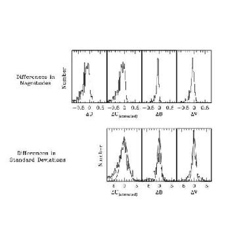
Figure 11: Histogram of magnitude differences between the Massey survey and the MCPS. Upper panels show the distributions of magnitude differences, lower panels show the distribution of magnitude differences in units of standard deviations (using the uncertainties associated with each star in the two catalogs). The curves plotted in the lower panels are Gaussians of $\sigma=2,1,1$ for $U,B,$ and $V$ respectively.

In Figure 11 we plot the distribution of magnitude differences for stars in Massey’s catalog and the MCPS that are in a magnitude range that is minimally affected by saturation and crowding ($B$ and $V>13.5$, $U<15$, and $B$ and $V<14.2$) and that have matches with separations less than 1 pixel (0.7 arcsec). The upper set of panels shows the $\Delta m$ distribution in magnitudes, the lower set shows the distribution in terms of standard deviations, propagating the uncertainty estimates from both catalogs. The histograms of $\Delta m$ for both $B$ and $V$ have a core that is actually slightly narrower than the Gaussian prediction, and wings that are larger, particularly in $V$. We suspect that the wings are due to zeropoint fluctuations between subscans that are somewhat larger than that suggested by the statistical errors of the photometric calibration (we will see more evidence of this effect later). The $U$ band data is fitted by a Gaussian that is twice as wide as expected, suggesting that the uncertainties are significantly underestimated. Again, we suggest that in large part this reflects zeropoint fluctuations among scans. For example, additional random fluctuations of 0.03 mag in the photometric zeropoints from subscan to subscan are sufficient to account for the widened distribution. This fluctuation in the zeropoints is consistent with the results of the internal comparison discussed previously.

3.2.2 Comparison to the OGLE Catalog

Zeropoint Calibration

The most extensive photometric data set available for comparison to our MCPS is that provided by the OGLE group (Udalski et al. (1998)). They have measured $B$, $V$, and $I$ magnitudes for stars along the central ridge line of the SMC. Again, we match stars between our catalog and theirs, and identify a magnitude regime where there appear to be no systematic problems. For this comparison we restrain the comparison to $B$ and $V>13.5$, a faint limit of 15 for $B$ and $V$, and 17 for $I$, and $|\Delta m|<0.2$. The mean photometric offsets are 0.011, 0.038, and 0.002 mag in $B$, $V$, and $I$ respectively. These are all within the internal uncertainties of our zeropoint calibration and in the opposite sense as the zeropoint differences resulting from the comparison to the Massey (2001) catalog. Again, we suggest that at least some part of the mean offsets are not due to photometric zero point errors, but to the systematic trend at fainter magnitudes (which is not due to calibration errors but rather to crowding). We conclude that our average, global photometric zeropoints are good to better than 0.03 mag.

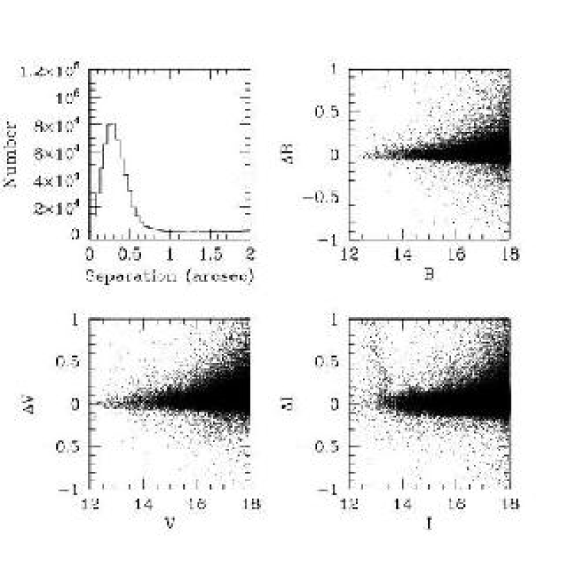
Figure 12: The comparison of the $BVI$ photometry from our survey with that from the OGLE survey. The upper left panel shows the distribution of matching separations between stars in the two surveys. The other three panels show the comparison of magnitudes.

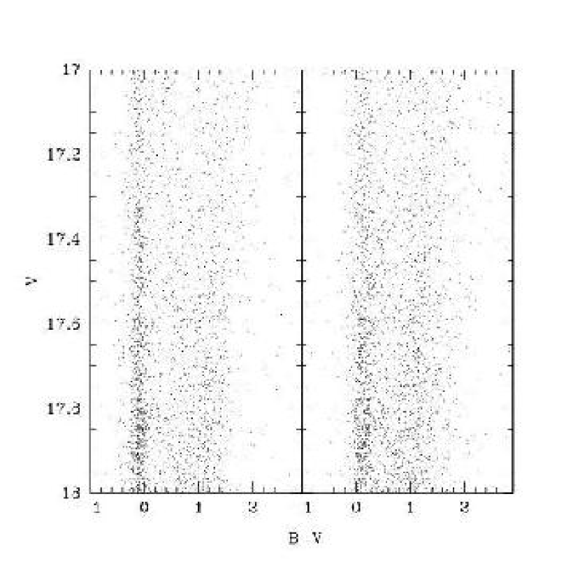
Figure 13: The color-magnitude diagram of fainter stars in common between the OGLE survey (left) and our survey (right) that have $\Delta V>$ 0.3 magnitudes (the faint tail).

In Figure 12 we show the same astrometric and photometric comparison that we did previously for the Massey (2001) catalog, except this time in $B,$ $V$, and $I$. We find again that the astrometric agreement is good to a fraction of a MCPS pixel. Regarding the magnitude comparison we find patterns similar to those seen previously. In the $I$ band comparison there is an upward tail at bright magnitudes. This is due to poorly modeled bright stars in the MCPS. These tails are not visible in the $B$ and $V$ comparisons because the photometry of stars with $B$ and $V<13.5$ was already replaced with the Massey (2001) photometry. We now replace the $I$ band photometry of suspect, bright stars ($I<13.5$) and an associated flag is set in the catalog — see §5). There are 1095 stars that are affected by this correction. We also see the asymmetry in residuals at faint magnitudes, however this time the tail is toward positive residuals. Comparing color-magnitude diagrams for stars with $\Delta m>0.3$ we find that the sequences appear tighter using the OGLE photometry (Figure 13). We conclude that the OGLE photometry is superior at the fainter magnitude levels. Nevertheless, the uncertainties in the MCPS catalog do include an approximation of the photometric uncertainties due to crowding. The $\Delta m$ distribution for the fainter stars is consistent, with the exception of a low-level tail toward positive residuals, with a Gaussian of unit dispersion and the additional scatter due to subscan-to-subscan photometric variations discussed earlier. Although the measurement uncertainties do reflect the crowding problems, any analysis that is sensitive to the details of the these errors should use artificial star tests (see Harris & Zaritsky (2001) for a discussion of those tests).

Color Terms

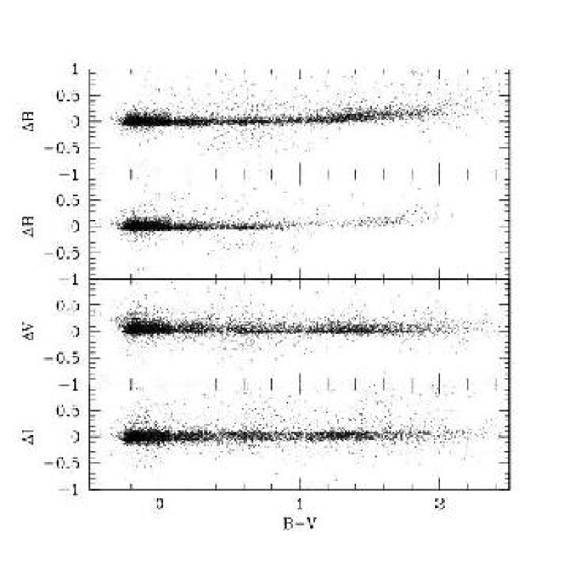
Figure 14: The residual magnitudes of stars matched between the OGLE and MCPS catalogs as a function of $B-V$ color. The uppermost panel shows the $B$ photometry for the same sample used in the lower two panels, while the second panel shows the comparison only for stars satisfying a brighter $B$ limit. In both of the upper two panels the color-dependency of the $B$ band residuals is evident.

Using the matched stars, we examine whether there are color-term variations between the two studies. From Figure 14, we conclude that the $V$ and $I$ photometry have no residual color-term dependences. In contrast, the $B$ photometry appears to have a systematic residual at red colors. Limiting the comparison to bright $B$ magnitudes, to avoid including many stars with large photometric residuals due to crowding, we still find the systematic color-dependent residual. Such a color-term is feasible because there are few standard stars at these extreme colors (Figure 1). However, the comparison to Massey’s catalog does not show such a problem (Figure 10). In that comparison, there is a photometry difference at $B-V\sim 1.2$, but by $B-V=1.5$ the $B$ photometry between the two studies agrees well (while the MCPS and OGLE photometry disagree by 0.1 mag at $B-V=1.5$). Because the comparison of the MCPS with these two surveys is inconclusive, and we have no further reason to suspect our photometry, we do not correct for the color term but caution that for the reddest stars there may be a $B$-band systematic error of $\sim 0.1$ mag in either our data or the OGLE data.

Verifying the Uncertainties

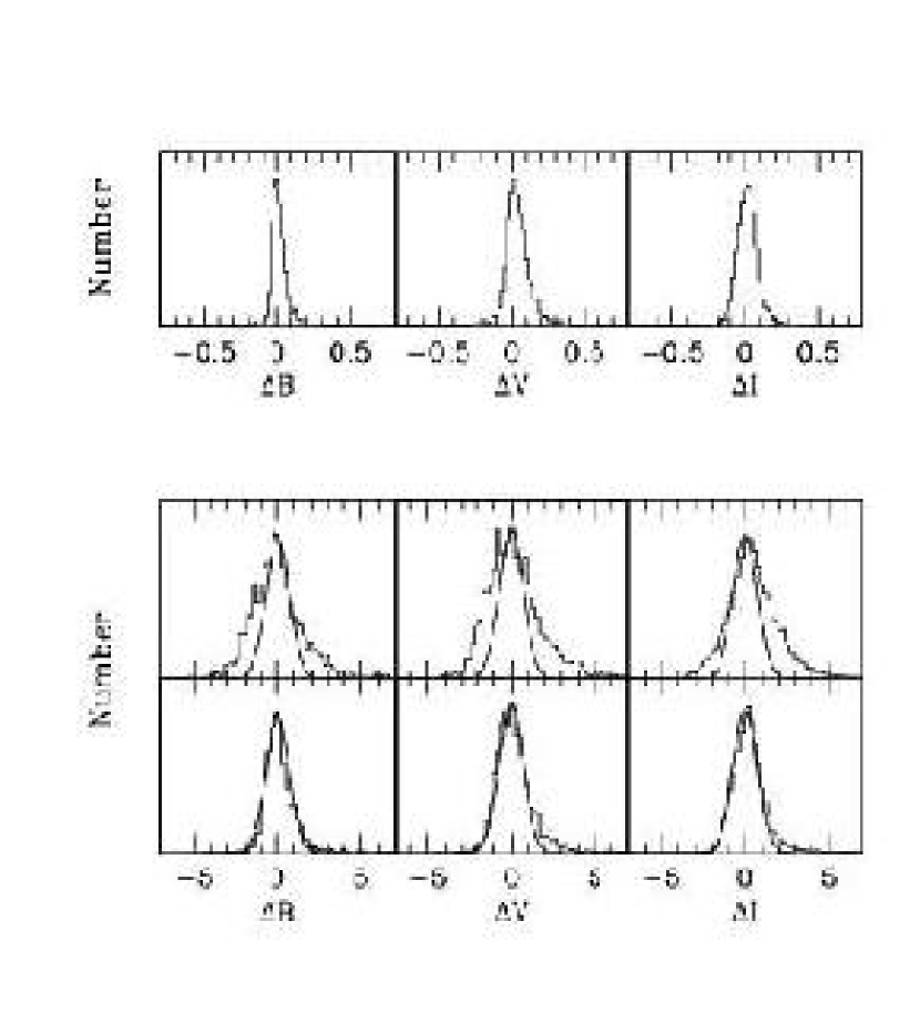
Figure 15: The distribution of magnitude differences between the OGLE survey and the MCPS. In the top panel we show the distribution in terms of magnitude differences for the three bands in common. In the middle set of panels is the distribution in terms of standard deviations and a Gaussian of unit dispersion is overplotted for comparison. In the lowest set of panels we show the same except we have added a dispersion of 0.03 mag to all uncertainties to model the scatter expected in the zeropoints from scan to scan.

Similar to our comparison to Massey’s catalog, we plot the distribution of magnitude differences for matched stars in units of magnitudes and standard deviations (Figure 15) for stars with astrometric differences $<$ 0.7 arcsec, $B$ and $V>13.5$, $B$ and $V<15$, and $I<16$. A Gaussian of width corresponding to the propagated uncertainties with an additional random photometric zeropoint uncertainty of 0.03 magnitudes agrees well with the distributions in all three bands. We conclude that the error estimates, with this small additional term due to uncertainties in the scan photometric zeropoints, describes the total uncertainties well at magnitudes where crowding does not play a role.

Spatially Varying Photometric Comparison

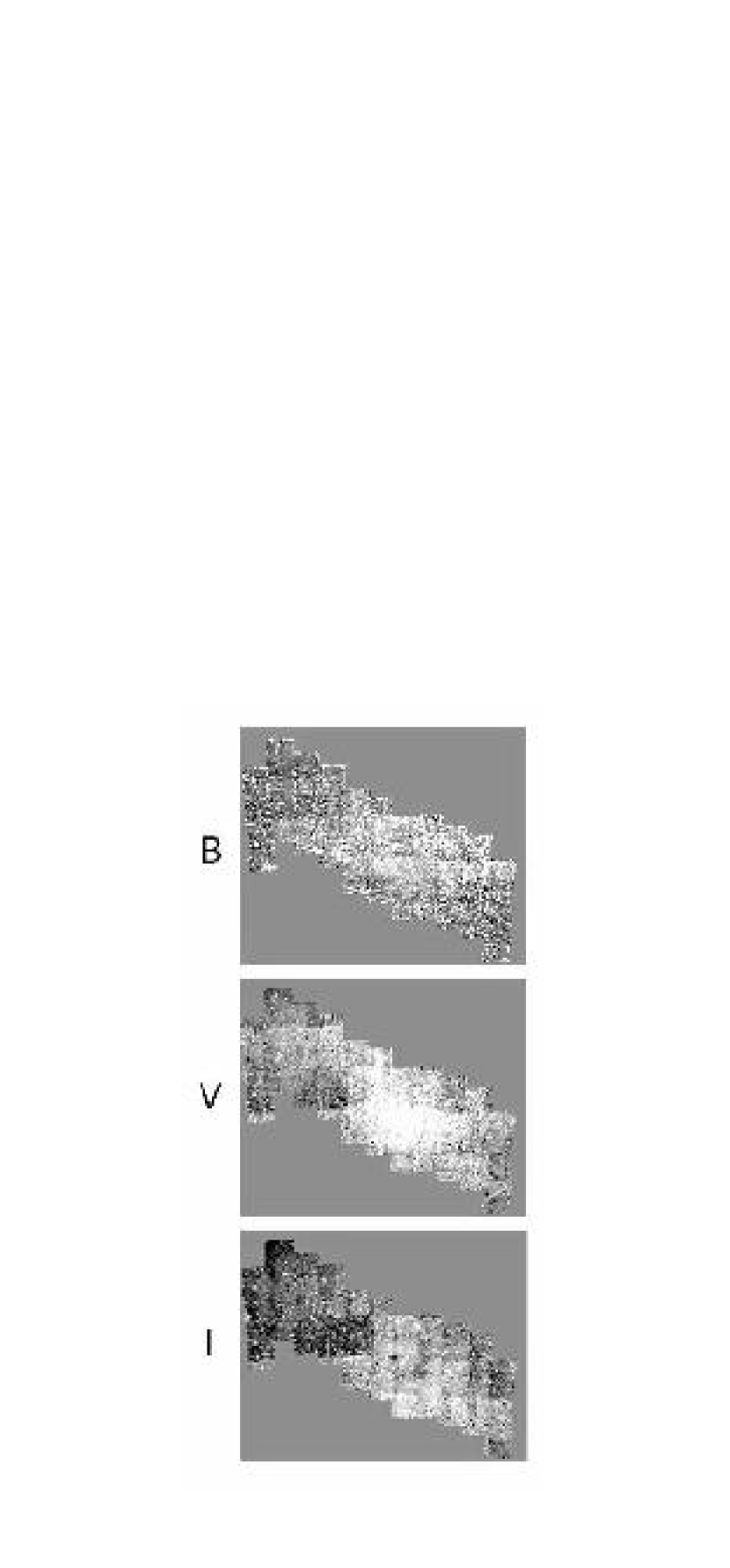
Figure 16: The spatial distribution of median magnitude differences between the OGLE survey and the MCPS for the three bands in common ($B$, $V$, and $I$). The OGLE survey concentrated on the ridge of the SMC and does not include the entire MCPS survey area. The grayscale covers the range $-0.1<\Delta m<0.1$.

The large sample of stars in common between MCPS and OGLE enables us to compare the photometry spatially over the area in common, and so determine whether there are problems on the scale of an individual scan or subscan (either in the MCPS or OGLE). In Figure 16 we present maps of the photometric offsets (median magnitude differences within square “pixels” for the matched stars used earlier to study global differences) for $B$, $V$, and $I$. Two types of spatial patterns are visible. The first consists either of vertical or horizontal striping. This striping is due to photometric errors in scans (MCPS has horizontal scans in this orientation, OGLE has vertical scans). Because different MCPS scans, even in the same filters, may come from runs separated by several years, it becomes difficult to obtain photometry that agrees to better than the internal calibration errors (typically $\sim 0.03$ mag). A horizontal edge is visible in the $I$-band, near the middle left of the image. Vertical edges are visible in the right half of the $I$-band panel. The difference across these edges is $\pm 0.05$ mag from the mean for the most noticeable edges. The second spatial pattern is the increasing discrepancy (especially in the $V$ band) toward the SMC center. This is almost certainly the effect of increasing crowding. At its worst, this offset appears to be 0.08 mag.

As the crowding increases beyond the ability of the data and software to disentangle, it becomes increasingly likely that fainter stars will contaminate the photometry of brighter stars (and that an increasing fraction of fainter stars will be lost). Therefore, the detected stars will become increasingly brighter (which is what is observed when comparing MCPS data to OGLE data in the crowded regions). OGLE is superior in this respect for several reasons: 1) their template images are taken in seeing as good as 0.8 arcsec, 2) their pixel scale (0.417 arcsec pixel^-1) is much better suited to the best seeing episodes than ours, and 3) they use repeat observations to cull unreliable photometry. In particular, our $V$ scan of the central region is not optimum. Obviously, higher quality data is desirable, but for some applications (such as the generation of synthetic color-magnitude diagrams) this effect can be included in the simulations and results only in a loss of information, not in a systematic error. Alternatively, investigators interested in the densest regions of the SMC may want to construct a hybrid catalog that uses OGLE data along the SMC ridge and MCPS data beyond the ridge. Users of the MCPS should be aware that there is a bias toward measuring a brighter magnitude for a star as one approaches the more heavily crowded fields.

3.2.3 Comparison to the DENIS Catalog

Finally, we compare our $I$-band photometry to that in the DENIS catalog. Although the DENIS catalog is primarily an IR catalog, it contains an $I$ band channel and Cioni et al. (2000) have extracted point-source catalogs in the regions of the Magellanic Clouds.

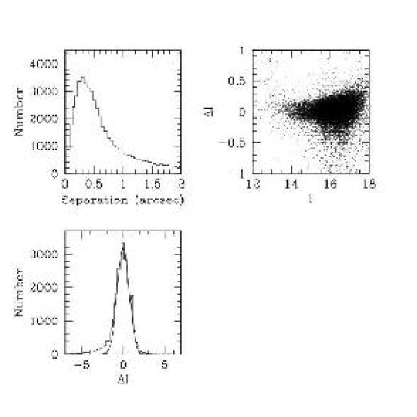
Figure 17: The comparison of DENIS $I$ band catalog with our data. The panel in the upper left illustrates the astrometric differences for matched stars. The panel in the upper right shows the difference in $I$ magnitudes as a function of $I$ magnitude. The panel in the lower left shows the differences normalized by the calculated uncertainty. A Gaussian of unit dispersion is overplotted for comparison.

We produce a similar comparison as to the Massey and OGLE catalogs, using a search aperture of 3.5 arcsec for matches. The distribution of astrometric and photometric differences for matched stars are plotted in Figure 17. In agreement with our previous results, we find that the astrometric accuracy is subpixel for the majority of the matches. The mean difference is 0.9 arcsec, but the mode is $\sim 0.3$ arcsec. Using only matched stars with positional offsets $<$ 1 pixel, the zeropoint difference between the two surveys is $-0.008$ mag. The distribution of photometry differences, in units of standard deviations, is entirely consistent with the propagated errors.

4 Extinction Properties

We developed a technique for fitting published stellar atmosphere models (Lejeune et al (1997)) to $U,B,V$, and $I$ photometry to measure the effective temperature, $T_{E}$, of the star and the line-of-sight extinction, A_V (Zaritsky (1999)). We found that the model fitting was least degenerate between $T_{E}$ and A_V for stars with derived temperatures in the ranges $5500{\ \rm K}\leq T_{E}\leq 6500{\ \ \rm K}$ and $12,000{\ \rm K}\leq T_{E}\leq 45000{\ \rm K}$. Therefore, we construct A_V maps of the SMC from the line-of-sight A_V measurements to the set of “cool” stars ($5500{\ \rm K}\leq T_{E}\leq 6500{\ \rm K}$) and the set of “hot” stars ($12000{\ \rm K}\leq T_{E}\leq 45000{\ \rm K}$) with good quality photometry ($\sigma_{U}<0.4$, $\sigma_{B}<0.2$, $\sigma_{V}<0.2$, $\sigma_{I}<0.2$) and good model fits ($\chi^{2}<3$). In addition to these criteria, we imposed a reddening-independent magnitude cut ($V<19.0+3.2\times(B-V)$).

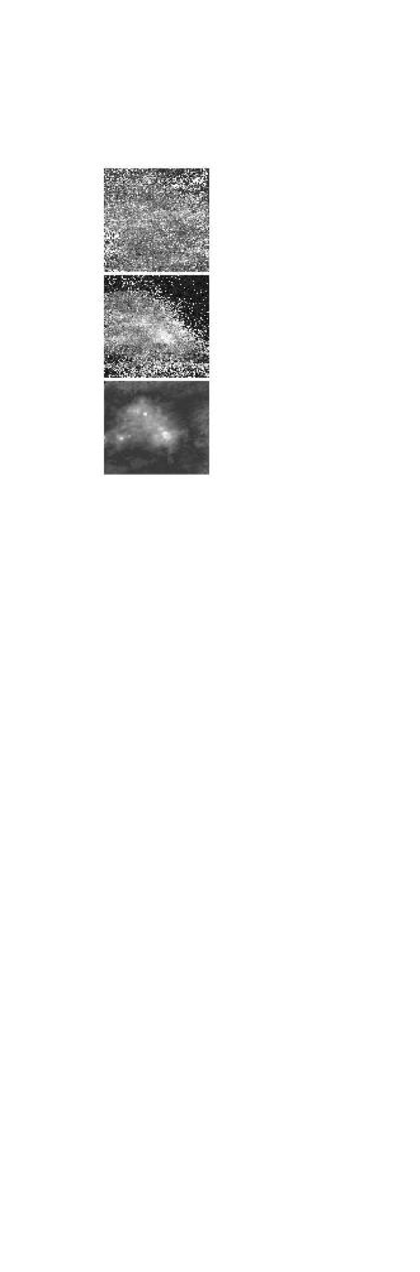
Figure 18: The spatial map of extinction values as derived for both the cooler, older stars ($5500{\ \rm K}\leq T_{E}\leq 6500{\ \rm K}$ ; upper panel) and the hotter, younger stars ($12000{\ \rm K}\leq T_{E}\leq 45000{\ \rm K}$; middle panel) for the entire survey region. The scale on the upper panel spans $-0.1\leq A_{V}\leq 0.4$, while the middle panel spanse $-0.1\leq A_{V}\leq 0.7$. The localized circular regions of apparent high extinction are globular clusters, which have some anomalous photometry because of their high stellar densities. Horizontal variations are due to scan-to-scan photometry differences of a few hundreths of a magnitude. The upper left and bottom of the map for the hot population are dominated by a small number of foreground stars. The lowest panel shows the 100$\mu$m emission image from IRAS (not on exactly the same scale).

The extinction maps (Figure  18) have lower signal-to-noise at large projected radii from the SMC because there are fewer stars at those radii. In particular, one should disregard the apparently low extinction toward the northwest in the “hot” population map because there are few such stars in this region. Because the recovery of A_V is quite sensitive to color, subtle differences in the scan photometry are highlighted in the extinction maps (in particular in that from the hot population). For example, a set of small photometric differences (0.03 mag in opposite senses in $B$ and $I$, so that $B-I$ has changed by 0.06 mag) creates an extinction discontinuity of the magnitude observed in the hot population map of Figure  18.

The principal coherent extinction structure within the body of the SMC is the increase in extinction in the hot star population along the ridge of the SMC (increasing to the southwest). This structure is not visible in the map from the colder stars indicating 1) that this structure may not be real, 2) that most cold stars in the SMC are in the foreground relative to the hot stars, or 3) that the dust may be highly localized near the younger stars, such that the lines-of-sight to background, colder stars are unlikely to contain much dust. We reject the first option because this ridge corresponds well to the morphology of the 100$\mu$ IRAS emission (Figure 18, bottom panel). The second option appears unlikely, simply because the colder, older stars are more likely to be more extended along the line-of-sight, both toward the foreground and background, than the younger stars. Therefore, we conclude that this observation implies that the dust along the SMC ridge line is spatially highly localized around the young, hot population.

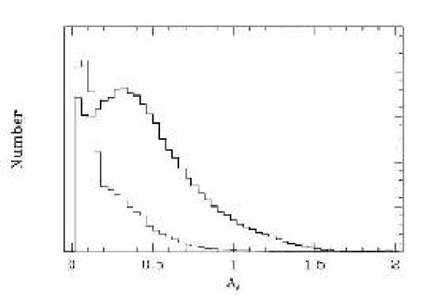
Figure 19: The distribution of extinction values for the two stellar populations using stars with model fits with $\chi^{2}\leq 3$ and the reddening-free magnitude cut described in the text. The narrow line represents the distribution of $A_{V}$ for the colder population and the bolder line for the hotter population. By construction $0\leq A_{V}<2$. The two histograms are normalized relative to each other, but there are 319,705 stars in the colder population and 136,268 in the hotter.

The A_V histograms of the two populations are shown in Figure 19. As we found for a region of the LMC (Zaritsky (1999)), the mean extinction is lower for the cooler populations (average A_V of 0.18 mag vs 0.46 mag for the cold vs. hot population, respectively). Given a foreground extinction of $\sim$ 0.15 mag toward the SMC (Bessel (1991)), the observed distribution of extinctions toward the colder stars suggests that there is little, if any, internal extinction in the SMC of the light from the distributed older population.

The principal difference between the SMC and LMC A_V histograms is the lack of a high-extinction tail for the cold stars in the SMC. For the LMC, this tail was interpreted to be the result of viewing roughly half of the colder stars through the irregular mid-plane dust layer associated with the hotter stars. We interpret the lack of such a tail in the SMC as an indication that the SMC has no pervasive dust layer that extincts light from background colder stars. This result is complementary to the explanation of the lack of a central ridge feature in the extinction map derived from the cold stars.

The localization of the significant extinction near massive stars, and the corresponding lack of significant extinction elsewhere in the SMC, has several causes. The low value of the global extinction is in part due to a dust-to-atomic gas ratio that is a factor of 30 below the Galactic value (Stanimirovic et al. (2000)). The lower dust abundance is related to the low observed abundance of CO in the SMC relative to the Galaxy or LMC. The global scarcity of CO is thought to arise because it is more easily photodissociated in the SMC (Rubio et al. (1993)). Lastly, the CO that is present in the SMC is concentrated along the central ridge, where most massive stars are found. We now have two cases (both LMC and SMC) for which detailed line-of-sight extinction measurements have shown significant differences ($\sim$ 0.3 mag) in the internal extinction of young and old stars. Typically, internal extinction corrections for galaxies are derived from tracers of recent star formation (for example, UV spectral slopes, $U-B$ colors, or H II region line ratios). Our results suggest that corrections derived from such tracers are likely to be too large if applied to the entire population of stars.

5 Catalog Supplements

The MCPS catalog for the SMC is presented as an ASCII text file (see Table 1 for an example, the full catalog is provided electronically). To enhance the usefulness of our catalog we augment the MCPS data in several ways. We have already described how we use data from Massey (2001) and Udalski et al. (1998) to correct our photometry for the brightest 0.02% of the cataloged stars ( $U,B,V$ for stars with $B$ or $V<13.5$ from Massey’s catalog and $I$ for stars with $I<13.5$ from OGLE). Column 11 of the catalog (see Table 1) is a quality flag that is the unique sum of several flags. Stars for which we replaced photometry with that from Massey’s catalog have a quality flag of $+1$. Stars for which we replaced photometry with that from OGLE have a quality flag of $+2$ (a star with a quality flag $=3$ has had its original photometry replaced with that from both Massey’s catalog and OGLE). Stars with measured magnitudes in $U,B,V$ and $I$ and $\sigma_{u}<0.4,\sigma_{b}<0.2,\sigma_{v}<0.2,$ and $\sigma_{I}<0.2$ are fit with stellar atmosphere models (§4). Those stars for which this fit is successful ($\chi^{2}<3$) are given a quality flag $+10$ and those which are unsuccessful are given a quality flag $+20$. Therefore, a star with a quality flag of 11, for example, had its $U,B$, and $V$ magnitudes replaced with those from Massey’s catalog and was successfully fit with a stellar atmosphere model.

We supplement the MCPS with IR data from the DENIS and Two Micron All Sky Survey (2MASS) surveys ($J$, $H$, and $K_{S}$, paired with their uncertainties, are in columns 12 - 17). We match stars in a manner similar to our previous comparisons, except we use an acceptance aperture of 1 arcsec and we have no magnitude criteria. If a star is matched only in 2MASS or DENIS data, then those data are used. If a star is matched to both catalogs, we use the average magnitude unless the IR magnitudes differed by more than 3$\sigma$ from each other in which case we do not use either data. We encourage investigators to examine other combinations of the catalogs, for example stars which are detected in the IR surveys but not in the optical may provide an interesting sample of highly obscured stars.

6 Summary

We are conducting a broad-band photometric survey of the Magellanic Clouds. Our intent is to provide these data to the community as quickly as possible and here we present the data for over 5 million stars in the $4.5^{\circ}\times 4^{\circ}$ survey area centered on the Small Magellanic Cloud. To enable potential users to understand these data we discuss various internal and external tests of the astrometry, photometry, and associated uncertainties. The catalog contains positions (right ascension and declination in J2000 coordinates) and $U$, $B$, $V$, and $I$ magnitudes and uncertainties in the Johnson-Kron-Cousins photometric system measured from our drift scan images. We augment this catalog with indications of the data quality. Lastly, we also provide the 2MASS/DENIS IR magnitudes matched to our data for ease of use of a dataset that is complete in $U$ to $K$ for 91,428 stars, provides incomplete coverage through the infrared bands for 183,751 stars, and at least partial optical coverage for 5,156,057 stars.

Using this catalog, we have constructed extinction maps for two stellar populations in the SMC. We find 1) that the bulk of the dust is concentrated along the ridge of the SMC, 2) that this dust is highly localized near the younger, hotter stars, 3) that aside from these regions of higher extinction, the average internal extinction in the SMC is consistent with zero, and 4) that the average extinction correction for the younger, hotter stars and the older, colder stars differs by about 0.3 mag. The latter conclusion is in agreement with what we found in the LMC (Zaritsky (1999)). On a more general vein, the two external galaxies for which we now have highly detailed maps of extinction as a function of stellar population both show significant differences in the extinction toward those populations. This difference, or at least the potential for this difference, should be considered when correcting the photometry of other galaxies for internal extinction. Generalizing, these results suggest that internal extinction corrections, which are commonly derived from tracers of recent star formation, are typically overestimated.

ACKNOWLEDGMENTS: DZ acknowledges financial support from an NSF grant (AST-9619576), a NASA LTSA grant (NAG-5-3501), and fellowships from the David and Lucile Packard Foundation and the Alfred P. Sloan Foundation. EKG acknowledges support from NASA through grant HF-01108.01-98A from the Space Telescope Science Institute.

Table 1: Sample of MCPS Catalog

RA	Dec	$U$	$\sigma_{U}$	$B$	$\sigma_{B}$	$V$	$\sigma_{V}$	$I$	$\sigma_{I}$	Flag	$J$	$\sigma_{J}$	$H$	$\sigma_{H}$	$K_{S}$	$\sigma_{K_{S}}$
0.398591	$-$74.09792	0.000	0.000	21.633	0.176	21.267	0.129	0.000	0.000	0	0.000	0.000	0.000	0.000	0.000	0.000
0.398591	$-$74.58766	0.000	0.000	22.394	0.165	22.446	0.223	0.000	0.000	0	0.000	0.000	0.000	0.000	0.000	0.000
0.398595	$-$73.92371	0.000	0.000	22.883	0.281	22.249	0.265	0.000	0.000	0	0.000	0.000	0.000	0.000	0.000	0.000
0.398595	$-$74.65561	19.804	0.201	20.845	0.095	20.715	0.075	20.625	0.160	10	0.000	0.000	0.000	0.000	0.000	0.000
0.398597	$-$74.01955	0.000	0.000	21.249	0.110	20.920	0.128	0.000	0.000	0	0.000	0.000	0.000	0.000	0.000	0.000
0.398598	$-$73.93850	0.000	0.000	21.362	0.144	21.120	0.133	0.000	0.000	0	0.000	0.000	0.000	0.000	0.000	0.000
0.398598	$-$74.32478	0.000	0.000	22.743	0.266	22.946	0.358	21.299	0.354	0	0.000	0.000	0.000	0.000	0.000	0.000
0.398600	$-$73.95302	17.380	0.058	17.819	0.033	17.927	0.030	17.996	0.042	10	0.000	0.000	0.000	0.000	0.000	0.000
0.398600	$-$74.01016	16.472	0.050	16.317	0.029	16.126	0.026	15.777	0.083	10	15.415	0.081	15.406	0.142	15.219	0.175
0.398603	$-$74.24788	0.000	0.000	22.945	0.278	21.286	0.080	19.681	0.080	0	0.000	0.000	0.000	0.000	0.000	0.000
0.398604	$-$74.37458	0.000	0.000	22.258	0.159	21.741	0.124	0.000	0.000	0	0.000	0.000	0.000	0.000	0.000	0.000
0.398604	$-$74.87499	0.000	0.000	22.628	0.214	21.801	0.119	21.172	0.230	0	0.000	0.000	0.000	0.000	0.000	0.000
0.398605	$-$74.74988	0.000	0.000	22.475	0.190	21.924	0.165	0.000	0.000	0	0.000	0.000	0.000	0.000	0.000	0.000
0.398606	$-$74.47800	18.868	0.071	18.837	0.058	18.059	0.023	17.108	0.048	10	16.350	0.111	15.792	0.164	0.000	9.999
0.398606	$-$74.78607	0.000	0.000	21.847	0.117	21.459	0.096	21.409	0.264	0	0.000	0.000	0.000	0.000	0.000	0.000
0.398607	$-$73.97942	0.000	0.000	21.651	0.112	20.748	0.091	19.818	0.089	0	0.000	0.000	0.000	0.000	0.000	0.000

References

- Alcock et al. (1997) Alcock, C., et al. 1997, ApJ, 486, 697
- Bessel (1991) Bessell, M.S. 1991, A&A, 242, L17
- Cioni et al. (2000) Cioni, M-R., et al., 2000, A&AS, 144, 235
- Epchtein et al. (1997) Epchtein, N., et al. 1997, Messenger, 87, 27
- Harris & Zaritsky (2001) Harris, J. & Zaritsky, D., in prep.
- Hatzidimitriou et al. (1989) Hatzidimitriou, D., & Hawkins, M.R.S. 1989, MNRAS, 241, 667
- Irwin et al. (1990) Irwin, M. J., Demers, S., & Kunkel, W.E. 1990, AJ, 99, 191
- Landolt (1983) Landolt, A.U. 1983, AJ, 88, 439
- Landolt (1992) Landolt, A.U. 1992, AJ, 104, 340
- Lejeune et al (1997) Lejeune, Th., Cuisinier, F., & Buser, R. 1997, A&AS, 125, 229
- Massey (2001) Massey, P. 2001, ApJS, submitted
- Palanque-Delabrouille et al. (1998) Palanque-Delabrouille, N., et al. 1998, A&A, 332, 1
- Rubio et al. (1993) Rubio, M., Lequeux, J., & Boulanger, F. 1993, A&A, 271, 9
- Smith et al. (2000) Smith, C., Leiton, R., & Pizarro, S. 2000, in “Stars, Gas, and Dust in Galaxies: Exploring the Links”, ASP Conference Proceedings vol. 221, (ed. D. Alloin, K. Olsen, & G. Galaz) (ASP: San Francisco), p. 83
- Stanimirovic et al. (2000) Sanimirovic, S., Staveley-Smith, L., van der Hulst, J.M., Bontekoe, Tj.R., Kester, D.J.M., and Jones, P.A. 2000, MNRAS, 315, 791
- Stetson (1987) Stetson, P. 1987, PASP, 99, 191
- Tucholke et al. (1996) Tucholke, H.-J., de Boer, K. S., & Seitter, W.C. 1996, A&A, 119, 91
- Udalski et al. (1998) Udalski, A., Szymanski, M., Kubiak, M., Pietrzynski, G., Wozniak, P., & Zebrun, K. 1998, Acta Astron., 48, 147
- van der Marel (2001) van der Marel, R.P., 2001, AJ, in press (astro-ph/0105340)
- Zaritsky (1999) Zaritsky, D., 1999, AJ, 195, 6801
- Zaritsky et al. (1997) Zaritsky, D., Harris, J., & Thompson, I. 1997, AJ, 114, 1002
- Zaritsky et al. (1996) Zaritsky, D., Shectman, S.A., & Bredthauer, G 1996, PASP, 108, 104
- Zaritsky et al. (2000) Zaritsky, D., Harris, J., Grebel, E.K., & Thompson, I. 2000, ApJ, 534, 53